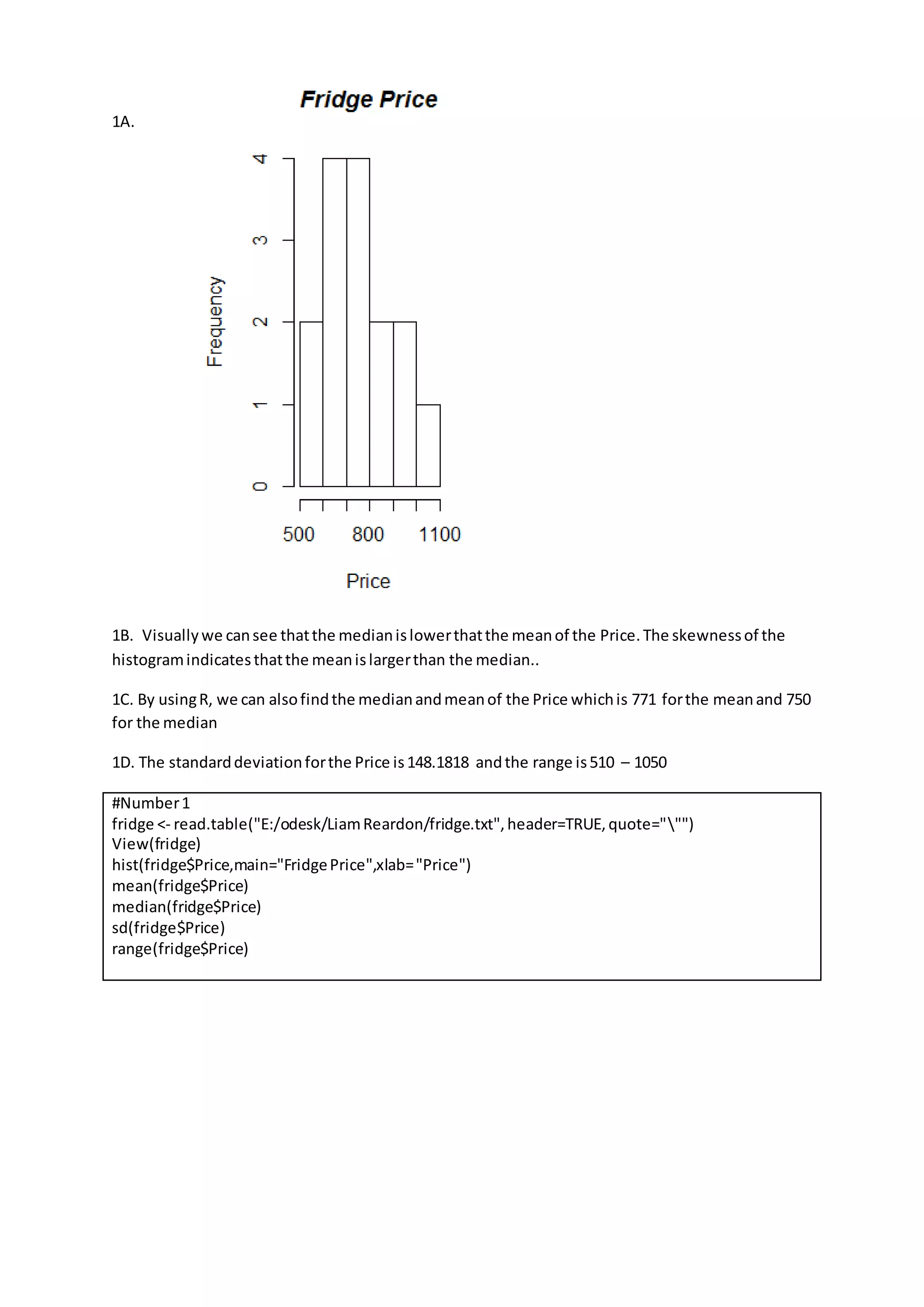
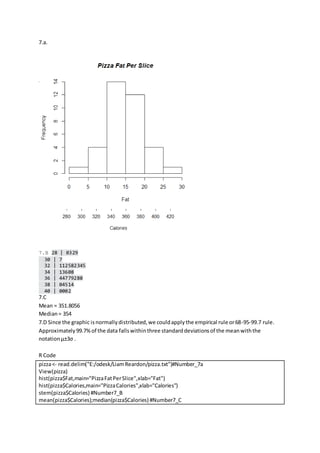
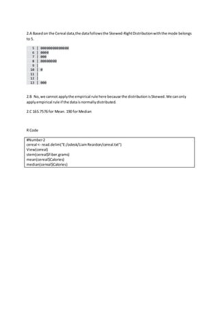
The document contains analyses of various datasets using R code. Key findings include: 1) For a fridge price dataset, the mean price is higher than the median price, indicating a skewed distribution. 2) Cereal fiber data follows a right-skewed distribution. The mean calories is higher than the median. 3) Changing data values by adding or multiplying a constant affects measures of central tendency but not measures of dispersion. 4) Analysis of lottery prize values finds the mean prize exceeds the ticket price, suggesting potential for profit. 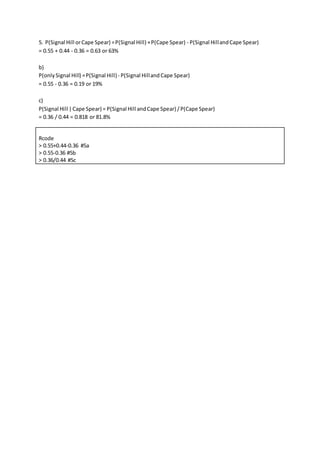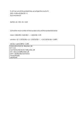5) Probability calculations are shown for events at two locations. 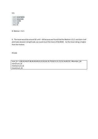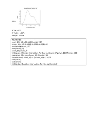6) Stem-and-leaf plot and measures of central tendency are presented for

1. 1A.
1B. Visuallywe cansee thatthe medianislowerthatthe meanof the Price.The skewnessof the
histogramindicatesthatthe meanislargerthan the median..
1C. By usingR, we can alsofindthe medianandmeanof the Price whichis 771 forthe meanand 750
for the median
1D. The standarddeviationforthe Price is148.1818 andthe range is510 – 1050
#Number1
fridge <- read.table("E:/odesk/LiamReardon/fridge.txt",header=TRUE,quote=""")
View(fridge)
hist(fridge$Price,main="FridgePrice",xlab="Price")
mean(fridge$Price)
median(fridge$Price)
sd(fridge$Price)
range(fridge$Price)

2. 2.A Basedon the Cereal data,the datafollowsthe Skewed-RightDistributionwiththe mode belongs
to 5.
5 | 00000000000000
6 | 0000
7 | 000
8 | 00000000
9 |
10 | 0
11 |
12 |
13 | 000
2.B No,we cannot applythe empirical rule here because the distributionisSkewed.We canonly
applyempirical rule if the dataisnormallydistributed.
2.C 165.7576 for Mean. 190 for Median
R Code
#Number2
cereal <- read.delim("E:/odesk/LiamReardon/cereal.txt")
View(cereal)
stem(cereal$Fiber.grams)
mean(cereal$Calories)
median(cereal$Calories)

3. 3.A. Mean = 3.375
Median= 3.5
Variance = 19.41071
StandardDeviation=4.405759
3.B [1] 6 9 5 2 -1 7 12 11
Mean = 6.375
Median= 6.5
Variance = 19.41071
StandardDeviation=4.405759
Comparedtoobservation(a) ,we got higherMeanand Medianbecause we incrementeach
observationby3 points butthe range betweenthe highestvalue andthe minimumvalue didn’t
change. Measure of dispersionwillbe the same if we addor decrease the whole dataat the same
time.Measure of dispersionincludesVariance andStandardDeviation.Meanwhile Mean,Median
and Mode are measure of Central Tendency.
3.C 13.5 27.0 9.0 -4.5 -18.0 18.0 40.5 36.0
Mean = 15.1875
Median= 15.75
Variance = 393.067
StandardDeviation=19.82592
Comparedto(a) , we got higherresultbecause we multiplyall the observation by4.5.Measure of
tendencyare increasedandMeasure of dispersionare alsoincreasedbecause the range between
each of data are largerdue to the multiply.
R Code
#Number3
num3A <- c(3,6,2,-1,-4,4,9,8)
mean(num3A);median(num3A);var(num3A);sd(num3A) #Number3A
num3B <- 3+num3A #Number3B
mean(num3B);median(num3B);var(num3B);sd(num3B)
num3C <- 4.5*num3A #Number3C
mean(num3C);median(num3C);var(num3C);sd(num3C)

4. 4. a. 12.45657 isthe meanof prize value
B. Yes,the meanexceedsourprice ticket,thiscouldyieldtomore profitif we buymore ticketfrom
Lotto 6/49.
Prize_Values<- c(14284257,441409.1,2430.9,76.20,10,5)
Number_Of_Winners<- c(0,1,150,9067,176083,127346)
Multiply<-Prize_Values*Number_Of_Winners
Mean_Result<- sum(Multiply)/sum(Number_Of_Winners)

5. 5. P(Signal Hill orCape Spear) =P(Signal Hill) +P(Cape Spear) - P(Signal HillandCape Spear)
= 0.55 + 0.44 - 0.36 = 0.63 or 63%
b)
P(onlySignal Hill) =P(Signal Hill)- P(Signal Hilland Cape Spear)
= 0.55 - 0.36 = 0.19 or 19%
c)
P(Signal Hill |Cape Spear) = P(Signal Hill andCape Spear) /P(Cape Spear)
= 0.36 / 0.44 = 0.818 or 81.8%
Rcode
> 0.55+0.44-0.36 #5a
> 0.55-0.36 #5b
> 0.36/0.44 #5c

6. 6.A.
4 | 03478999
5 | 0112345
6 | 1256
7 | 69
8 | 9
B. Median= 51.5
6. The meanwouldbe around50 until – 60 because we foundthatthe Medianis51.5 andstem-leaf
plotlooksskewed.UsingRcode,we couldresultthe meanof 56.04545 . So the meanrating ishigher
than the median.
R Code
num_6 <- c(40,43,44,47,48,49,49,49,61,62,65,66,76,79,50,51,51,52,53,54,89,55) #Number_6A
stem(num_6)
median(num_6)
mean(num_6)

7. 7.a.
7.B
7.B 28 | 0329
30 | 7
32 | 112582345
34 | 13608
36 | 44779288
38 | 04514
40 | 0002
7.C
Mean = 351.8056
Median= 354
7.D Since the graphic isnormallydistributed,we couldapplythe empirical rule or68-95-99.7 rule.
Approximately99.7%of the data fallswithinthree standarddeviationsof the meanwiththe
notation μ±3σ .
R Code
pizza<- read.delim("E:/odesk/LiamReardon/pizza.txt")#Number_7a
View(pizza)
hist(pizza$Fat,main="PizzaFatPerSlice",xlab="Fat")
hist(pizza$Calories,main="PizzaCalories",xlab="Calories")
stem(pizza$Calories) #Number7_B
mean(pizza$Calories);median(pizza$Calories) #Number7_C

8. 8. A. To get the assumptiontrue forfoursuspect,we multiplyforeachevent.
0.98^4 = .9224 or 92.24%
B. The chance of correct is 98% forthe machine.Soto get incorrectresult,we substractthe chance
from100%l
1 - 0.98^4 = .0776 or 7.76%
So,7.76% of the resultwill yieldtoincorrect
R Code
#Number_8
0.98^4 #Number_8A
1- (0.98)^4 #Number_8B

9. 9. a) If we sumall the probabilities,we will getthe resultof 1
0.05 + 0.20+x+0.35+0.10 =1
So,X must be 0.3
(b) P(X> 3) = P(X= 4) = 0.10
(c) Findthe meannumberof cheesecakessold,andthe standarddeviation
mean= (0)(0.05) + (1)(0.20) + ... + (4)(0.10) = 2.25
variance = (0 - 2.25)²(0.05) + (1 - 2.25)²(0.20) + ...+ (4-2.25)²(0.10) = 1.0875
std dev= sqrt(1.0875) = 1.043
0.05+0.20+0.35+0.10 #Number_9A
0.7 + 0.3
list("P(X>3)=P(X=4)=0.1") #Number_9B
x9 <- c(0,1,2,3,4)#Number_9C
px9 <- c(0.05,0.20,0.3,0.35,0.1)
mean(x9*px9)
sd(x9*px9)

10. 10. A.
B. E(x) = 1.27
C. Var(x) = 1.6671
SD(x) = 1.295029
#Number10
xnum_10 <- c(0,1,2,3,4,5,6)#number_10A
pxnum_10 <- c(0.32,0.35,0.18,0.08,0.04,0.02,0.01)
plot(density(pxnum_10))
plot(pxnum_10)
xnum_10*pxnum_10
list(Expected_Number_Interupttion_Per_Day=sum(xnum_10*pxnum_10)) #Number_10B
meanxnum_10<- mean(xnum_10) #Number_10C
varcalc <- sum((xnum_10)^2* (pxnum_10)) - (1.27)^2
sum(varcalc)
sqrt(varcalc)
list(Standard_Deviation_Interupption_Per_Day=sqrt(varcalc))

11. 11.n = 9 ( numberof householdsselected)
p = .73 ( probabilitythata householdownsadigital camera)
x = numberof householdsoutof 9 owninga digital camera
a)
P(x=2) = 0.002006756
b)
P( at most1) = 0.0001931818
c)
P( at least1) = 0.9999924
d) Mean = 6.57
StandardDeviation=1.331878
E)P(X>=350) = 1
P0<-(factorial(9))/((factorial(0)*factorial(9-0)))*(0.73^0) * ((1-0.73)^(9-0))
P1<-(factorial(9))/((factorial(1)*factorial(9-1)))*(0.73^1) * ((1-0.73)^(9-1))
P2<-(factorial(9))/((factorial(2)*factorial(9-2)))*(0.73^2) * ((1-0.73)^(9-2))
P350<-(factorial(450))/((factorial(0)*factorial(450))) *(0.73^0) * ((1-0.73)^(450-0))
m <-(1-0.73)^(450-0)
1-m #Number_11E
9*0.73
stdev_num11<-9*0.73
list("Number11A"=P2, "Number11B"= P0+P1, "Number11C"= 1-P0,"Number11DMean" =
9*0.73,"Number11D StandardDeviation"=sqrt(9*0.73*(1-0.73))) #Number_11A