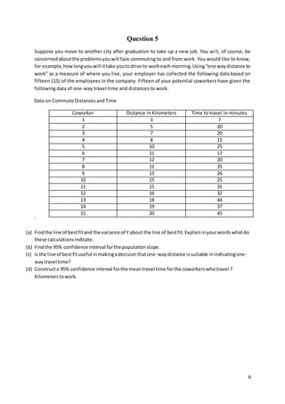
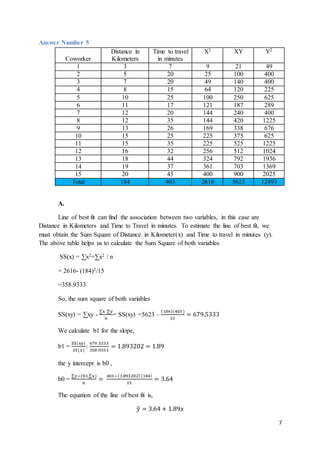
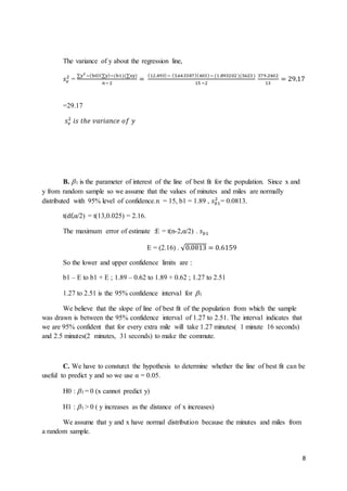
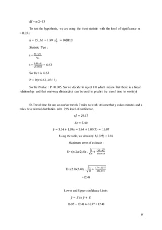
SlideShare a Scribd company logo
1
Contents
Question 1 ...................................................................................................................................1
Answer number 1 ..................................................................................................................... 1
Question 2: ..................................................................................................................................2
Answer number 2 ..................................................................................................................... 2
Question 3 ...................................................................................................................................3
Answer number 3 ..................................................................................................................... 3
Question 4: ..................................................................................................................................4
Answer Number 4..................................................................................................................... 4
Question 5 ...................................................................................................................................6
Answer Number 5..................................................................................................................... 7
Question 1
1. Many people sleeplate onthe weekendstomake upfor “shortnights”duringthe work week.The
Better Sleep council reports that 61% of us get more than 7 hours of sleep per night on the
weekend.A randomsample of 350 adults found that 235 had more than 7 hours of sleep each night
lastweekend.Atthe 0.05 level of significance,does this evidence show that more than 61% sleep 7
hours or more per night on the weekend?
Answer number 1
1. p is the proportion of adults who get more than 7 hours of sleep each night on weekends.
Hypothesis :
Ho: p = P(7+ hours of sleep) ≤ 0.61 (no more than 61% or equal to 61%)
Ha: p > 0.61 (more than 61%)
The n =350 which is greater than 20 so we use the standard normal z.
np and nq is also greater than 5 . np=(350)(0.61) = 213.5 ; nq = (350)(0.39) = 136.5.
p is expected to be normally distributed.
p’=
𝑥
𝑛
=
235
350
= 0.671
z’ =
𝑝′
−𝑝
√
𝑝𝑞
𝑛
=
0.671 −0.61
√
(0.61)(0.39)
350
=
0.061
√0.0006797
=
0.061
0.0261
= 2.34
By using the standard normal probability table, the pvalue is 1 - .9904 = 0.0096
Or, by using calculator, we get the p value = 0.0096
2
So the Pvalue is smaller than The level of signifiance is  = 0.05 .
Conclusion :
We reject Ho . There is sufficient reason to conclude that the proportion of adults in the
sampled population who are getting more than 7 hours of sleep nightly on weekends is
significantly higher than 61% at the 0.05 level of significance
Question 2:
For years, many large companies in Melbourne have used a reputable employment agency for
testing perspective employees. The employment selection test used has historically resulted in scores
of normally distributed about a mean of 82 and a standard deviation of 8. A competitor has developed
a new psychoanalytic test that it claims to be quicker and easier to administer and therefore less
expensive. The competitor claims that its test results are the same as those obtained by the reputable
agency test. Many of the large companies, facing the financial crunch, are considering a change to cut
costs. However, they are unwilling to change if the competitor firm’s test results have a different
mean value. An independent testing firm tested 36 prospective employees with the Brown test. A
sample mean of 70 resulted. Determine the p value associated with this hypothesis test. (Assume
population standard deviation to be 8).
Answer number 2
The population mean . The mean of all test scores using the Brown Agency test.
Hypothesis :
Ho:  = 82 (Test results have the same mean)
Ha:   82 (Test results have different mean)
𝞼 is known. If the brown test scores are distributed the same as the kelley test scores, they
will be normally distributed and the sampling distribution will be normal for all sample sizes.
The standard normal probability distribution and the test statistic :
z’ =
𝑋̅− 
𝑠/√ 𝑛
will be used with 𝞼 = 8
Level of significance is not used because the question asks for Pvalue only, so there will
be no decision making for this case.
n= 36 ; 𝑋̅ = 79
z’ =
𝑋̅− 
𝑠/√ 𝑛
; z’ =
79−82
8/√36
=
−3
1.3333
= -2.25
The alternative hypothesis is two tailed test, we must find the probability associated with
both tails.
z’ = -2.25, the value of | 𝑧′| = 2.25.
3
The Pvalue = 2 * P (z >2.25) = 2* (0.5000 – 0.4878) = 2(0.0122) = 0.0244
The Pvalue for the hypothesis test is 0.0255. Each individual company now will decide
whether to continue to use the Kelley Agency’s Servies or change to Brown Agency. We can
decide based on the hypothesis it if the case have the level of significance.
Question 3
On a popularself-image test that results in normally distributed scores, the mean score for public-
assistance recipientsisexpectedtobe 65. A randomsample of 28 publicassistance recipientsinNTG
is given the test. They achieve a mean score of 62.1, and their scores have a standard deviation of
5.83. Do the NTG publicassistance recipients test differently on average, than what is expected, at
the 0.02 level of significance?
Answer number 3
 is the mean self image test score for all NTG public assistance recipients.
The hypothesis for the null hypothesis and alternative hypothesis
Ho:  = 65 (mean is 65)
Ha:   65 (mean is different from 65)
For this case,the assumption of normal distribution has been satisfied based on the case. The level of
significance is  = 0.02. So we use t’ for the statistical test.
n= 28, 𝑋̅= 62.1 and s = 5.83 .
The value of the test statistics :
t’ =
𝑋̅− 
𝑠/√ 𝑛
t’ =
62.1− 65
5.83/√28
=
−2.9
1.1018
= -2.632
=-2.63
Because the alternative hypothesis express the difference of mean, so we use both tail to calculate the
pvalue for the test statistic.
P = P(t –2.63) + P(t 2.63) = 2  P(t 2.63), with df = 27.
with t=2.63 and df = 27,
The Pvalue is P = 0.0139.
Conclusion:
4
The Pvalue is smaller than the level of significance (P = 0.0139 <  = 0.02). So we reject Ho . At the
level of significance 2% or0.02,we have sufficient evidence to conclude that the NTG recipients tests
significantly different on average fromthe expected 65
Question 4:
College students have regularly insisted on freedom of choice when they register for tutorial classes.
In one semester there were seven tutorials offered at different times in the Decision making unit.
Table below provides the number of students who selected each of the seven tutorial classes:
Tutorial 1 2 3 4 5 6 7 Total
No. of
Students
18 12 25 23 8 19 14 119
Does the data indicate that students have a preference for certain tutorials or do they indicate that each
tutorial was equally likely to be chosen? Explain your answer fully. Show all your workings clearly.
Answer Number 4 :
If there are no preference for certain tutorials for the students, then we expect that 119 students in total
are equally distributed for each tutorial. We test hypothesis using 95% confidence level.
Parameter of interest : Preference each tutorials.
Hypothesis :
H0 : There was no preference shown
H1 : There was a preference shown.
119 students in total is a random sample of population of all student who register for the tutorial.
We are using the chi-square distribution for the statistical test with df = 6, α=0.05
𝜒2 = ∑
(𝑂−𝐸)2
𝐸
𝜒2 = ∑
(18−17)2
17
+
(18−17)2
17
+
(12−17)2
17
+
(25−17)2
17
+
(23−17)2
17
+
(8−17)2
17
+
(19−17)2
17
+
(14−17)2
17
𝜒2 =
12+(−5)2+(82)+(62)+(−92)+(2)2+(−32)
17
𝜒2 =
1+25+64+36+81+4+9
17
𝜒2 =
220
17
= 𝟏𝟐. 𝟗𝟒
Pvalue = P(𝜒2 > 12.94 | 𝑑𝑓 = 6) . By using calculator, the pvalue = 0.044
5
Decision : For this case we Reject H0 because pvalue is smaller than the level of significance of 5%
or 0.05. The decision shows us that there was a preference shown, but we cannot decide yet what
preference is relevance for this occasion, it could be the time preference or teacher preference.
6
Question 5
Suppose you move to another city after graduation to take up a new job. You will, of course, be
concernedaboutthe problemsyouwill face commuting to and from work. You would like to know,
for example,howlongyouwill ittake youtodrive to workeach morning.Using“one waydistance to
work” as a measure of where you live, your employer has collected the following data based on
fifteen (15) of the employees in the company. Fifteen of your potential coworkers have given the
following data of one-way travel time and distances to work.
Data on Commute DistancesandTime
Coworker Distance in Kilometers Time to travel in minutes
1 3 7
2 5 20
3 7 20
4 8 15
5 10 25
6 11 17
7 12 20
8 12 35
9 13 26
10 15 25
11 15 35
12 16 32
13 18 44
14 19 37
15 20 45
`
(a) Findthe line of bestfitand the variance of Y about the line of bestfit.Explaininyourwordswhatdo
these calculationsindicate.
(b) Findthe 95% confidence interval forthe populationslope.
(c) Is the line of bestfituseful inmakingadecisionthatone-waydistance issuitable inindicatingone-
waytravel time?
(d) Constructa 95% confidence interval forthe meantravel time forthe coworkerswhotravel 7
Kilometerstowork.
7
Answer Number 5
Coworker
Distance in
Kilometers
Time to travel
in minutes
X2 XY Y2
1 3 7 9 21 49
2 5 20 25 100 400
3 7 20 49 140 400
4 8 15 64 120 225
5 10 25 100 250 625
6 11 17 121 187 289
7 12 20 144 240 400
8 12 35 144 420 1225
9 13 26 169 338 676
10 15 25 225 375 625
11 15 35 225 525 1225
12 16 32 256 512 1024
13 18 44 324 792 1936
14 19 37 361 703 1369
15 20 45 400 900 2025
Total 184 403 2616 5623 12493
A.
Line of best fit can find the association between two variables, in this case are
Distance in Kilometers and Time to Travel in minutes. To estimate the line of best fit, we
must obtain the Sum Square of Distance in Kilometer(x) and Time to travel in minutes (y).
The above table helps us to calculate the Sum Square of both variables
SS(x) = ∑x2=∑x2 / n
= 2616- (184)2/15
=358.9333
So, the sum square of both variables
SS(xy) = ∑xy -
∑x .∑y
𝑛
= SS(xy) =5623 –
(184)(403)
15
= 679.5333
We calculate b1 for the slope,
b1 =
SS(xy)
𝑆𝑆(𝑥)
:
679 .5333
358 .9333
= 1.893202 = 1.89
the y intercept is b0 ,
b0 =
∑y−(b1.∑x)
𝑛
=
403−(1.893202)(184)
15
= 3.64
The equation of the line of best fit is,
𝑦̂ = 3.64 + 1.89𝑥
8
The variance of y about the regression line,
𝑠 𝑒
2
=
∑y2
−(b0)(∑y)−(b1)(∑xy)
𝑛−2
=
(12,493)− (3.643387)(403)− (1.893202 )(5623 )
15 −2
379.2402
13
= 29.17
=29.17
𝑠 𝑒
2
𝑖𝑠 𝑡ℎ𝑒 𝑣𝑎𝑟𝑖𝑎𝑛𝑐𝑒 𝑜𝑓 𝑦
B. 1 is the parameter of interest of the line of best fit for the population. Since x and
y from random sample so we assume that the values of minutes and miles are normally
distributed with 95% level of confidence.n = 15, b1 = 1.89 , 𝑠 𝑏1
2
= 0.0813.
t(df,α/2) = t(13,0.025) = 2.16.
The maximum error of estimate :E = t(n-2,α/2) . 𝑠 𝑏1
E = (2.16) . √0.0813 = 0.6159
So the lower and upper confidence limits are :
b1 – E to b1 + E ; 1.89 – 0.62 to 1.89 + 0.62 ; 1.27 to 2.51
1.27 to 2.51 is the 95% confidence interval for 1
We believe that the slope of line of best fit of the population from which the sample
was drawn is between the 95% confidence interval of 1.27 to 2.51. The interval indicates that
we are 95% confident that for every extra mile will take 1.27 minutes( 1 minute 16 seconds)
and 2.5 minutes(2 minutes, 31 seconds) to make the commute.
C. We have to consturct the hypothesis to determine whether the line of best fit can be
useful to predict y and so we use α = 0.05.
H0 : 1 = 0 (x cannot predict y)
H1 : 1 > 0 ( y increases as the distance of x increases)
We assume that y and x have normal distribution because the minutes and miles from
a random sample.
9
df = n-2=13
To test the hypothesis, we are using the t test statistic with the level of significance α
= 0.05.
n = 15 , b1 = 1.89 𝑠 𝑏1
2
= 0.0813
Statistic Test :
t =
𝑏1−1
𝑠 𝑏1
t =
1.89−0
√0.0813
= 6.63
So the t is 6.63
P = P(t>6.63, df=13)
So the Pvalue : P <0.005. So we decide to reject H0 which means that there is a linear
relationship and that one-way distance(x) can be used to predict the travel time to work(y)
D. Travel time for one co-worker travels 7 miles to work. Assume that y values minutes and x
miles have normal distribution with 95% level of confidence.
𝑠 𝑒
2 = 29.17
𝑆𝑒 = 5.40
𝑦̂ = 3.64 + 1.89𝑥 = 3.64 + 1.89(7) = 16.87
Using the table, we obrain t(13,0.025) = 2.16
Maximum error of estimate :
E= t(n-2,α/2).Se . √1
𝑛
+
(𝑥0−𝑥)̂2
358.933
E= (2.16(5.40) . √
1
15
+
(7−12.272
358.933
=12.48
Lower and Upper confidence Limits
𝑦̂ − 𝐸 𝑡𝑜 𝑦̂ + 𝐸
16.87 – 12.48 to 16.87 + 12.48
10
So we have 4.39 to 29.35 with 95% confidence interval. This indicates that the co-worker
travel times for commuters who travel 7 miles is between 4.39 minutes (4 minutes, 23 seconds) and
29.35 minutes(29 minutes,21 seconds)

More Related Content

What's hot

Week8 Live Lecture for Final Exam
Week8 Live Lecture for Final ExamWeek8 Live Lecture for Final Exam
Week8 Live Lecture for Final Exam
Brent Heard
 
Decision Tree and Bayesian Classification
Decision Tree and Bayesian ClassificationDecision Tree and Bayesian Classification
Decision Tree and Bayesian Classification
Komal Kotak
 
Decision tree for Predictive Modeling
Decision tree for Predictive ModelingDecision tree for Predictive Modeling
Decision tree for Predictive Modeling
Edureka!
 
Decision tree
Decision treeDecision tree
Decision tree
Venkata Reddy Konasani
 
Les5e ppt 07
Les5e ppt 07Les5e ppt 07
Les5e ppt 07
Subas Nandy
 
Probability module 1
Probability module 1Probability module 1
Probability module 1
Richard Paulino
 
352735322 rsh-qam11-tif-03-doc
352735322 rsh-qam11-tif-03-doc352735322 rsh-qam11-tif-03-doc
352735322 rsh-qam11-tif-03-doc
Firas Husseini
 
Biomath12
Biomath12Biomath12
Biomath12
guruppkn11
 
Week8 finalexamlivelecture 2010december
Week8 finalexamlivelecture 2010decemberWeek8 finalexamlivelecture 2010december
Week8 finalexamlivelecture 2010december
Brent Heard
 
Math 221 Massive Success / snaptutorial.com
Math 221 Massive Success / snaptutorial.comMath 221 Massive Success / snaptutorial.com
Math 221 Massive Success / snaptutorial.com
Stephenson164
 
Slide3.ppt
Slide3.pptSlide3.ppt
Slide3.pptbutest
 
165662191 chapter-03-answers-1
165662191 chapter-03-answers-1165662191 chapter-03-answers-1
165662191 chapter-03-answers-1
Firas Husseini
 
Decision tree
Decision treeDecision tree
Decision tree
Varun Jain
 
Brand Equity: Dish Home of Nepal
Brand Equity: Dish Home of NepalBrand Equity: Dish Home of Nepal
Brand Equity: Dish Home of Nepal
Sajeeb Shrestha, PhD
 
Module 3 statistics
Module 3   statisticsModule 3   statistics
Module 3 statistics
dionesioable
 
Rsh qam11 ch07 ge
Rsh qam11 ch07 geRsh qam11 ch07 ge
Rsh qam11 ch07 ge
Firas Husseini
 

What's hot (17)

Week8 Live Lecture for Final Exam
Week8 Live Lecture for Final ExamWeek8 Live Lecture for Final Exam
Week8 Live Lecture for Final Exam
 
Decision Tree and Bayesian Classification
Decision Tree and Bayesian ClassificationDecision Tree and Bayesian Classification
Decision Tree and Bayesian Classification
 
Decision tree for Predictive Modeling
Decision tree for Predictive ModelingDecision tree for Predictive Modeling
Decision tree for Predictive Modeling
 
Decision tree
Decision treeDecision tree
Decision tree
 
Les5e ppt 07
Les5e ppt 07Les5e ppt 07
Les5e ppt 07
 
Probability module 1
Probability module 1Probability module 1
Probability module 1
 
352735322 rsh-qam11-tif-03-doc
352735322 rsh-qam11-tif-03-doc352735322 rsh-qam11-tif-03-doc
352735322 rsh-qam11-tif-03-doc
 
Biomath12
Biomath12Biomath12
Biomath12
 
Week8 finalexamlivelecture 2010december
Week8 finalexamlivelecture 2010decemberWeek8 finalexamlivelecture 2010december
Week8 finalexamlivelecture 2010december
 
Math 221 Massive Success / snaptutorial.com
Math 221 Massive Success / snaptutorial.comMath 221 Massive Success / snaptutorial.com
Math 221 Massive Success / snaptutorial.com
 
Slide3.ppt
Slide3.pptSlide3.ppt
Slide3.ppt
 
165662191 chapter-03-answers-1
165662191 chapter-03-answers-1165662191 chapter-03-answers-1
165662191 chapter-03-answers-1
 
Ch08(1)
Ch08(1)Ch08(1)
Ch08(1)
 
Decision tree
Decision treeDecision tree
Decision tree
 
Brand Equity: Dish Home of Nepal
Brand Equity: Dish Home of NepalBrand Equity: Dish Home of Nepal
Brand Equity: Dish Home of Nepal
 
Module 3 statistics
Module 3   statisticsModule 3   statistics
Module 3 statistics
 
Rsh qam11 ch07 ge
Rsh qam11 ch07 geRsh qam11 ch07 ge
Rsh qam11 ch07 ge
 

Similar to ANSWERS

Solution manual for design and analysis of experiments 9th edition douglas ...
Solution manual for design and analysis of experiments 9th edition   douglas ...Solution manual for design and analysis of experiments 9th edition   douglas ...
Solution manual for design and analysis of experiments 9th edition douglas ...
Salehkhanovic
 
Confidence Level and Sample Size
Confidence Level and Sample SizeConfidence Level and Sample Size
Confidence Level and Sample Size
Emilio Fer Villa
 
Week 7 Lecture
Week 7 LectureWeek 7 Lecture
Week 7 Lecture
Brent Heard
 
Section 8 Ensure Valid Test and Survey Results Trough .docx
Section 8 Ensure Valid Test and Survey Results Trough .docxSection 8 Ensure Valid Test and Survey Results Trough .docx
Section 8 Ensure Valid Test and Survey Results Trough .docx
kenjordan97598
 
227_ch7-hw-soln.pdf
227_ch7-hw-soln.pdf227_ch7-hw-soln.pdf
227_ch7-hw-soln.pdf
CamilaTinampay
 
Chapter9
Chapter9Chapter9
1624.pptx
1624.pptx1624.pptx
1624.pptx
Jyoti863900
 
Probability unit2.pptx
Probability unit2.pptxProbability unit2.pptx
Probability unit2.pptx
SNIGDHABADIDA2127755
 
Two Means, Independent Samples
Two Means, Independent SamplesTwo Means, Independent Samples
Two Means, Independent Samples
Long Beach City College
 
Estimating a Population Standard Deviation or Variance
Estimating a Population Standard Deviation or VarianceEstimating a Population Standard Deviation or Variance
Estimating a Population Standard Deviation or Variance
Long Beach City College
 
Estimating a Population Standard Deviation or Variance
Estimating a Population Standard Deviation or Variance Estimating a Population Standard Deviation or Variance
Estimating a Population Standard Deviation or Variance
Long Beach City College
 
Role of estimation in statistics
Role of estimation in statisticsRole of estimation in statistics
Role of estimation in statistics
Nadeem Uddin
 
Hypothesis Testing techniques in social research.ppt
Hypothesis Testing techniques in social research.pptHypothesis Testing techniques in social research.ppt
Hypothesis Testing techniques in social research.ppt
Solomonkiplimo
 
Chisquare Test
Chisquare Test Chisquare Test
Chisquare Test
Manas Mondal
 
Accuracy and errors
Accuracy and errorsAccuracy and errors
Accuracy and errors
SHELAMIE SANTILLAN
 
Week8 livelecture2010
Week8 livelecture2010Week8 livelecture2010
Week8 livelecture2010
Brent Heard
 
Hypothesis Testing on bus. analytics 101
Hypothesis Testing on bus. analytics 101Hypothesis Testing on bus. analytics 101
Hypothesis Testing on bus. analytics 101
Abdullah Amin
 
Final examexamplesapr2013
Final examexamplesapr2013Final examexamplesapr2013
Final examexamplesapr2013
Brent Heard
 
VCE Physics: Dealing with numerical measurments
VCE Physics: Dealing with numerical measurmentsVCE Physics: Dealing with numerical measurments
VCE Physics: Dealing with numerical measurments
Andrew Grichting
 

Similar to ANSWERS (20)

Solution manual for design and analysis of experiments 9th edition douglas ...
Solution manual for design and analysis of experiments 9th edition   douglas ...Solution manual for design and analysis of experiments 9th edition   douglas ...
Solution manual for design and analysis of experiments 9th edition douglas ...
 
Confidence Level and Sample Size
Confidence Level and Sample SizeConfidence Level and Sample Size
Confidence Level and Sample Size
 
Week 7 Lecture
Week 7 LectureWeek 7 Lecture
Week 7 Lecture
 
Section 8 Ensure Valid Test and Survey Results Trough .docx
Section 8 Ensure Valid Test and Survey Results Trough .docxSection 8 Ensure Valid Test and Survey Results Trough .docx
Section 8 Ensure Valid Test and Survey Results Trough .docx
 
227_ch7-hw-soln.pdf
227_ch7-hw-soln.pdf227_ch7-hw-soln.pdf
227_ch7-hw-soln.pdf
 
Chapter9
Chapter9Chapter9
Chapter9
 
1624.pptx
1624.pptx1624.pptx
1624.pptx
 
Probability unit2.pptx
Probability unit2.pptxProbability unit2.pptx
Probability unit2.pptx
 
Two Means, Independent Samples
Two Means, Independent SamplesTwo Means, Independent Samples
Two Means, Independent Samples
 
Estimating a Population Standard Deviation or Variance
Estimating a Population Standard Deviation or VarianceEstimating a Population Standard Deviation or Variance
Estimating a Population Standard Deviation or Variance
 
Estimating a Population Standard Deviation or Variance
Estimating a Population Standard Deviation or Variance Estimating a Population Standard Deviation or Variance
Estimating a Population Standard Deviation or Variance
 
Role of estimation in statistics
Role of estimation in statisticsRole of estimation in statistics
Role of estimation in statistics
 
Hypothesis Testing techniques in social research.ppt
Hypothesis Testing techniques in social research.pptHypothesis Testing techniques in social research.ppt
Hypothesis Testing techniques in social research.ppt
 
Chisquare Test
Chisquare Test Chisquare Test
Chisquare Test
 
Accuracy and errors
Accuracy and errorsAccuracy and errors
Accuracy and errors
 
Chapter09
Chapter09Chapter09
Chapter09
 
Week8 livelecture2010
Week8 livelecture2010Week8 livelecture2010
Week8 livelecture2010
 
Hypothesis Testing on bus. analytics 101
Hypothesis Testing on bus. analytics 101Hypothesis Testing on bus. analytics 101
Hypothesis Testing on bus. analytics 101
 
Final examexamplesapr2013
Final examexamplesapr2013Final examexamplesapr2013
Final examexamplesapr2013
 
VCE Physics: Dealing with numerical measurments
VCE Physics: Dealing with numerical measurmentsVCE Physics: Dealing with numerical measurments
VCE Physics: Dealing with numerical measurments
 

More from Yogi Sarumaha

Assignment_01_F2015 stats
Assignment_01_F2015 statsAssignment_01_F2015 stats
Assignment_01_F2015 statsYogi Sarumaha
 
Final Case study answer
Final Case study answerFinal Case study answer
Final Case study answerYogi Sarumaha
 

More from Yogi Sarumaha (6)

Assignment_01_F2015 stats
Assignment_01_F2015 statsAssignment_01_F2015 stats
Assignment_01_F2015 stats
 
answer
answeranswer
answer
 
Topic
TopicTopic
Topic
 
Final Case study answer
Final Case study answerFinal Case study answer
Final Case study answer
 
MoreCheating(1)
MoreCheating(1)MoreCheating(1)
MoreCheating(1)
 
leslie
leslieleslie
leslie
 

ANSWERS

  • 1. 1 Contents Question 1 ...................................................................................................................................1 Answer number 1 ..................................................................................................................... 1 Question 2: ..................................................................................................................................2 Answer number 2 ..................................................................................................................... 2 Question 3 ...................................................................................................................................3 Answer number 3 ..................................................................................................................... 3 Question 4: ..................................................................................................................................4 Answer Number 4..................................................................................................................... 4 Question 5 ...................................................................................................................................6 Answer Number 5..................................................................................................................... 7 Question 1 1. Many people sleeplate onthe weekendstomake upfor “shortnights”duringthe work week.The Better Sleep council reports that 61% of us get more than 7 hours of sleep per night on the weekend.A randomsample of 350 adults found that 235 had more than 7 hours of sleep each night lastweekend.Atthe 0.05 level of significance,does this evidence show that more than 61% sleep 7 hours or more per night on the weekend? Answer number 1 1. p is the proportion of adults who get more than 7 hours of sleep each night on weekends. Hypothesis : Ho: p = P(7+ hours of sleep) ≤ 0.61 (no more than 61% or equal to 61%) Ha: p > 0.61 (more than 61%) The n =350 which is greater than 20 so we use the standard normal z. np and nq is also greater than 5 . np=(350)(0.61) = 213.5 ; nq = (350)(0.39) = 136.5. p is expected to be normally distributed. p’= 𝑥 𝑛 = 235 350 = 0.671 z’ = 𝑝′ −𝑝 √ 𝑝𝑞 𝑛 = 0.671 −0.61 √ (0.61)(0.39) 350 = 0.061 √0.0006797 = 0.061 0.0261 = 2.34 By using the standard normal probability table, the pvalue is 1 - .9904 = 0.0096 Or, by using calculator, we get the p value = 0.0096
  • 2. 2 So the Pvalue is smaller than The level of signifiance is  = 0.05 . Conclusion : We reject Ho . There is sufficient reason to conclude that the proportion of adults in the sampled population who are getting more than 7 hours of sleep nightly on weekends is significantly higher than 61% at the 0.05 level of significance Question 2: For years, many large companies in Melbourne have used a reputable employment agency for testing perspective employees. The employment selection test used has historically resulted in scores of normally distributed about a mean of 82 and a standard deviation of 8. A competitor has developed a new psychoanalytic test that it claims to be quicker and easier to administer and therefore less expensive. The competitor claims that its test results are the same as those obtained by the reputable agency test. Many of the large companies, facing the financial crunch, are considering a change to cut costs. However, they are unwilling to change if the competitor firm’s test results have a different mean value. An independent testing firm tested 36 prospective employees with the Brown test. A sample mean of 70 resulted. Determine the p value associated with this hypothesis test. (Assume population standard deviation to be 8). Answer number 2 The population mean . The mean of all test scores using the Brown Agency test. Hypothesis : Ho:  = 82 (Test results have the same mean) Ha:   82 (Test results have different mean) 𝞼 is known. If the brown test scores are distributed the same as the kelley test scores, they will be normally distributed and the sampling distribution will be normal for all sample sizes. The standard normal probability distribution and the test statistic : z’ = 𝑋̅−  𝑠/√ 𝑛 will be used with 𝞼 = 8 Level of significance is not used because the question asks for Pvalue only, so there will be no decision making for this case. n= 36 ; 𝑋̅ = 79 z’ = 𝑋̅−  𝑠/√ 𝑛 ; z’ = 79−82 8/√36 = −3 1.3333 = -2.25 The alternative hypothesis is two tailed test, we must find the probability associated with both tails. z’ = -2.25, the value of | 𝑧′| = 2.25.
  • 3. 3 The Pvalue = 2 * P (z >2.25) = 2* (0.5000 – 0.4878) = 2(0.0122) = 0.0244 The Pvalue for the hypothesis test is 0.0255. Each individual company now will decide whether to continue to use the Kelley Agency’s Servies or change to Brown Agency. We can decide based on the hypothesis it if the case have the level of significance. Question 3 On a popularself-image test that results in normally distributed scores, the mean score for public- assistance recipientsisexpectedtobe 65. A randomsample of 28 publicassistance recipientsinNTG is given the test. They achieve a mean score of 62.1, and their scores have a standard deviation of 5.83. Do the NTG publicassistance recipients test differently on average, than what is expected, at the 0.02 level of significance? Answer number 3  is the mean self image test score for all NTG public assistance recipients. The hypothesis for the null hypothesis and alternative hypothesis Ho:  = 65 (mean is 65) Ha:   65 (mean is different from 65) For this case,the assumption of normal distribution has been satisfied based on the case. The level of significance is  = 0.02. So we use t’ for the statistical test. n= 28, 𝑋̅= 62.1 and s = 5.83 . The value of the test statistics : t’ = 𝑋̅−  𝑠/√ 𝑛 t’ = 62.1− 65 5.83/√28 = −2.9 1.1018 = -2.632 =-2.63 Because the alternative hypothesis express the difference of mean, so we use both tail to calculate the pvalue for the test statistic. P = P(t –2.63) + P(t 2.63) = 2  P(t 2.63), with df = 27. with t=2.63 and df = 27, The Pvalue is P = 0.0139. Conclusion:
  • 4. 4 The Pvalue is smaller than the level of significance (P = 0.0139 <  = 0.02). So we reject Ho . At the level of significance 2% or0.02,we have sufficient evidence to conclude that the NTG recipients tests significantly different on average fromthe expected 65 Question 4: College students have regularly insisted on freedom of choice when they register for tutorial classes. In one semester there were seven tutorials offered at different times in the Decision making unit. Table below provides the number of students who selected each of the seven tutorial classes: Tutorial 1 2 3 4 5 6 7 Total No. of Students 18 12 25 23 8 19 14 119 Does the data indicate that students have a preference for certain tutorials or do they indicate that each tutorial was equally likely to be chosen? Explain your answer fully. Show all your workings clearly. Answer Number 4 : If there are no preference for certain tutorials for the students, then we expect that 119 students in total are equally distributed for each tutorial. We test hypothesis using 95% confidence level. Parameter of interest : Preference each tutorials. Hypothesis : H0 : There was no preference shown H1 : There was a preference shown. 119 students in total is a random sample of population of all student who register for the tutorial. We are using the chi-square distribution for the statistical test with df = 6, α=0.05 𝜒2 = ∑ (𝑂−𝐸)2 𝐸 𝜒2 = ∑ (18−17)2 17 + (18−17)2 17 + (12−17)2 17 + (25−17)2 17 + (23−17)2 17 + (8−17)2 17 + (19−17)2 17 + (14−17)2 17 𝜒2 = 12+(−5)2+(82)+(62)+(−92)+(2)2+(−32) 17 𝜒2 = 1+25+64+36+81+4+9 17 𝜒2 = 220 17 = 𝟏𝟐. 𝟗𝟒 Pvalue = P(𝜒2 > 12.94 | 𝑑𝑓 = 6) . By using calculator, the pvalue = 0.044
  • 5. 5 Decision : For this case we Reject H0 because pvalue is smaller than the level of significance of 5% or 0.05. The decision shows us that there was a preference shown, but we cannot decide yet what preference is relevance for this occasion, it could be the time preference or teacher preference.
  • 6. 6 Question 5 Suppose you move to another city after graduation to take up a new job. You will, of course, be concernedaboutthe problemsyouwill face commuting to and from work. You would like to know, for example,howlongyouwill ittake youtodrive to workeach morning.Using“one waydistance to work” as a measure of where you live, your employer has collected the following data based on fifteen (15) of the employees in the company. Fifteen of your potential coworkers have given the following data of one-way travel time and distances to work. Data on Commute DistancesandTime Coworker Distance in Kilometers Time to travel in minutes 1 3 7 2 5 20 3 7 20 4 8 15 5 10 25 6 11 17 7 12 20 8 12 35 9 13 26 10 15 25 11 15 35 12 16 32 13 18 44 14 19 37 15 20 45 ` (a) Findthe line of bestfitand the variance of Y about the line of bestfit.Explaininyourwordswhatdo these calculationsindicate. (b) Findthe 95% confidence interval forthe populationslope. (c) Is the line of bestfituseful inmakingadecisionthatone-waydistance issuitable inindicatingone- waytravel time? (d) Constructa 95% confidence interval forthe meantravel time forthe coworkerswhotravel 7 Kilometerstowork.
  • 7. 7 Answer Number 5 Coworker Distance in Kilometers Time to travel in minutes X2 XY Y2 1 3 7 9 21 49 2 5 20 25 100 400 3 7 20 49 140 400 4 8 15 64 120 225 5 10 25 100 250 625 6 11 17 121 187 289 7 12 20 144 240 400 8 12 35 144 420 1225 9 13 26 169 338 676 10 15 25 225 375 625 11 15 35 225 525 1225 12 16 32 256 512 1024 13 18 44 324 792 1936 14 19 37 361 703 1369 15 20 45 400 900 2025 Total 184 403 2616 5623 12493 A. Line of best fit can find the association between two variables, in this case are Distance in Kilometers and Time to Travel in minutes. To estimate the line of best fit, we must obtain the Sum Square of Distance in Kilometer(x) and Time to travel in minutes (y). The above table helps us to calculate the Sum Square of both variables SS(x) = ∑x2=∑x2 / n = 2616- (184)2/15 =358.9333 So, the sum square of both variables SS(xy) = ∑xy - ∑x .∑y 𝑛 = SS(xy) =5623 – (184)(403) 15 = 679.5333 We calculate b1 for the slope, b1 = SS(xy) 𝑆𝑆(𝑥) : 679 .5333 358 .9333 = 1.893202 = 1.89 the y intercept is b0 , b0 = ∑y−(b1.∑x) 𝑛 = 403−(1.893202)(184) 15 = 3.64 The equation of the line of best fit is, 𝑦̂ = 3.64 + 1.89𝑥
  • 8. 8 The variance of y about the regression line, 𝑠 𝑒 2 = ∑y2 −(b0)(∑y)−(b1)(∑xy) 𝑛−2 = (12,493)− (3.643387)(403)− (1.893202 )(5623 ) 15 −2 379.2402 13 = 29.17 =29.17 𝑠 𝑒 2 𝑖𝑠 𝑡ℎ𝑒 𝑣𝑎𝑟𝑖𝑎𝑛𝑐𝑒 𝑜𝑓 𝑦 B. 1 is the parameter of interest of the line of best fit for the population. Since x and y from random sample so we assume that the values of minutes and miles are normally distributed with 95% level of confidence.n = 15, b1 = 1.89 , 𝑠 𝑏1 2 = 0.0813. t(df,α/2) = t(13,0.025) = 2.16. The maximum error of estimate :E = t(n-2,α/2) . 𝑠 𝑏1 E = (2.16) . √0.0813 = 0.6159 So the lower and upper confidence limits are : b1 – E to b1 + E ; 1.89 – 0.62 to 1.89 + 0.62 ; 1.27 to 2.51 1.27 to 2.51 is the 95% confidence interval for 1 We believe that the slope of line of best fit of the population from which the sample was drawn is between the 95% confidence interval of 1.27 to 2.51. The interval indicates that we are 95% confident that for every extra mile will take 1.27 minutes( 1 minute 16 seconds) and 2.5 minutes(2 minutes, 31 seconds) to make the commute. C. We have to consturct the hypothesis to determine whether the line of best fit can be useful to predict y and so we use α = 0.05. H0 : 1 = 0 (x cannot predict y) H1 : 1 > 0 ( y increases as the distance of x increases) We assume that y and x have normal distribution because the minutes and miles from a random sample.
  • 9. 9 df = n-2=13 To test the hypothesis, we are using the t test statistic with the level of significance α = 0.05. n = 15 , b1 = 1.89 𝑠 𝑏1 2 = 0.0813 Statistic Test : t = 𝑏1−1 𝑠 𝑏1 t = 1.89−0 √0.0813 = 6.63 So the t is 6.63 P = P(t>6.63, df=13) So the Pvalue : P <0.005. So we decide to reject H0 which means that there is a linear relationship and that one-way distance(x) can be used to predict the travel time to work(y) D. Travel time for one co-worker travels 7 miles to work. Assume that y values minutes and x miles have normal distribution with 95% level of confidence. 𝑠 𝑒 2 = 29.17 𝑆𝑒 = 5.40 𝑦̂ = 3.64 + 1.89𝑥 = 3.64 + 1.89(7) = 16.87 Using the table, we obrain t(13,0.025) = 2.16 Maximum error of estimate : E= t(n-2,α/2).Se . √1 𝑛 + (𝑥0−𝑥)̂2 358.933 E= (2.16(5.40) . √ 1 15 + (7−12.272 358.933 =12.48 Lower and Upper confidence Limits 𝑦̂ − 𝐸 𝑡𝑜 𝑦̂ + 𝐸 16.87 – 12.48 to 16.87 + 12.48
  • 10. 10 So we have 4.39 to 29.35 with 95% confidence interval. This indicates that the co-worker travel times for commuters who travel 7 miles is between 4.39 minutes (4 minutes, 23 seconds) and 29.35 minutes(29 minutes,21 seconds)