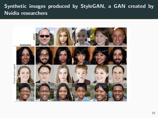
The document provides a comprehensive overview of neural networks, detailing their origins, architectures, and applications in machine learning, particularly focusing on deep learning and generative adversarial networks (GANs). Key topics include the structure of neural networks, the learning process through backpropagation and optimization algorithms, and the variations in activation functions. It also introduces advanced models like convolutional and recurrent neural networks, highlighting their unique characteristics and contributions to deep learning.

1. Neural Networks
Xiaocheng Li
Imperial College Business School, Imperial College London
xiaocheng.li@imperial.ac.uk
1

2. Neural Network
The model of neural network in
machine learning was first inspired
by Biological neural networks
Figure From ”Texture of the
Nervous System of Man and the
Vertebrates” by Santiago Ramon y
Cajal: It illustrates the diversity of
neuronal morphologies in the
auditory cortex.
2

3. Neural Networks in Machine Learning
The study of neural network model in machine learning can be dated
back to 1960s and gains great popularity in the past decade
The notion of “deep learning” refers to neural networks with large
number of parameters
The neural network model mimics the operations of a human brain to
recognize relationships between vast amounts of data
Reference for this lecture: Elements of Statistical Learning, Chapter 11,
Jerome H. Friedman, Robert Tibshirani, and Trevor Hastie
If you want to study deep learning in depth (far beyond the scope of our
module), refer to the deep learning book:
https://www.deeplearningbook.org/ and also all the online
tutorials/courses
3

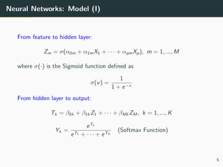
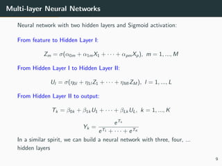
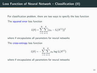
4. Neural Networks: Model (Single Hidden Layer)
Figure 11.2 from ESL:
Schematic of a single hidden
layer, feed-forward neural
network.
Input: (X1, ..., Xp) ∈ Rp
Output:
(Y1, ..., YK ) ∈ [0, 1]K
, the
probability of the sample’s
label being k = 1, ..., K
Hidden layer:
(Z1, ..., ZM ) ∈ RM
4

5. Neural Networks: Model (I)
From feature to hidden layer:
Zm = σ(α0m + α1mX1 + · · · + αpmXp), m = 1, ..., M
where σ(·) is the Sigmoid function defined as
σ(v) =
1
1 + e−v
From hidden layer to output:
Tk = β0k + β1k Z1 + · · · + βMk ZM , k = 1, ..., K
Yk =
eTk
eT1 + · · · + eTK
(Softmax Function)
5

6. Neural Networks: Model (II)
Parameters for neural networks:
{α0m, α1m, ..., αpm : m = 1, ..., M} M(p + 1) weights
{β0k , β1k , ..., βMk : k = 1, ..., K} K(M + 1) weights
For the testing/inference phase of a neural network
• Compute Z = (Z1, ..., ZM ) from input variable X = (X1, ..., Xp)
• Compute Y = (Y1, ..., YK ) from Z = (Z1, ..., ZM )
• Assign the label of the sample according to the largest Yk
6

7. Basic Variants of the Neural Network Model (I)
For a regression problem, the top (output) layer has only one neuron
(K = 1)
Y = γ0 + γ1Z1 + · · · + γM ZM
In this way, the top layer can be viewed as a simple linear regression
In neural networks, we will first do a linear transformation for the
variables in a certain layer and then go through the activation function
such as Sigmoid function σ(·) to obtain the variable on the next layer
The role of the activation function: Non-linearity!
7

8. Basic Variants of the Neural Network Model (II)
Another popular choice for the activation function is the ReLU function
(positive part function):
r(v) = max(0, v)
One-hidden-layer neural network with ReLU activation:
From feature to hidden layer:
Zm = r(α0m + α1mX1 + · · · + αpmXp), m = 1, ..., M
From hidden layer to output:
Tk = β0k + β1k Z1 + · · · + βMk Zm, k = 1, ..., K
Yk =
eTk
eT1 + · · · + eTK
8

9. Multi-layer Neural Networks
Neural network with two hidden layers and Sigmoid activation:
From feature to Hidden Layer I:
Zm = σ(α0m + α1mX1 + · · · + αpmXp), m = 1, ..., M
From Hidden Layer I to Hidden Layer II:
Ul = σ(η0l + η1l Z1 + · · · + ηMl ZM ), l = 1, ..., L
From Hidden Layer II to output:
Tk = β0k + β1k U1 + · · · + βLk UL, k = 1, ..., K
Yk =
eTk
eT1 + · · · + eTK
In a similar spirit, we can build a neural network with three, four, ...
hidden layers
9

10. Visualizing Neural Network
https://playground.tensorflow.org/
You can basically visualize everything related to a (small) neural network
model
10

11. Learning of Neural Networks
The learning of neural networks falls into the general framework of
empirical risk minimization, and we will use optimization algorithms to
find the optimal parameters for a neural network model
Two questions:
• Loss function
• Learning of the weights/parameters
11

12. Loss Function of Neural Network – Classification (I)
For classification problem, denote the output Yk , k = 1, ..., K as a
function of input variable X
Yk = fk (X)
Training data (Y (i)
, X(i)
), i = 1, ..., N
Remark: The one-hot encoding of the output variable
Y (i)
= (yi1, ..., yiK )
where yik = 1 if the i-th sample’s label is k, and yik = 0 otherwise
12

13. Loss Function of Neural Network – Classification (II)
For classification problem, there are two ways to specify the loss function
The squared error loss function
L(θ) =
N
X
i=1
K
X
k=1
(yik − fk (X(i)
))2
where θ encapsulates all parameters for neural networks
The cross-entropy loss function
L(θ) = −
N
X
i=1
K
X
k=1
yik log fk (X(i)
)
where θ encapsulates all parameters for neural networks
13

14. Loss Function of Neural Network – Regression
For regression problem, there is only one output neuron Y as a function
of input variable X
Y = f (X)
Training data (Y (i)
, X(i)
), i = 1, ..., N
The squared error loss function
L(θ) =
N
X
i=1
(Y (i)
− f (X(i)
))2
where θ encapsulates all parameters for neural networks
14

15. Learning of the Parameters
Gradient descent algorithm:
Randomly initialize θ0
For t = 1, ...
θt = θt−1 − γt∇L(θt−1)
Stop if certain criteria is met
γt : step size in optimization algorithm, also known as learning rate
15

16. Back Propagation
The number of parameters can be large for neural network model. In
other words, the parameter θ is a high-dimensional vector.
Back Propagation
• An efficient way to compute the gradient layer by layer, from output
layer all the way back to the input layer
• Mathematically, it is simply the chain rule for computing gradient. A
composite function h(θ) = f (g(θ)) where x ∈ R, then
h0
(θ) = f 0
(g(θ))g0
(θ)
16
NOT COMING FROM THIS SLIDE ONWARDSSS

17. Back Propagation for the One-hidden-layer Neural Network
The gradient of the loss function for the i-th sample
Compute the gradient from the top layer to the bottom layer
Reuse the computed gradient of the previous layer
17

18. Stochastic Gradient Descent
Neural network models usually have a large number of training samples
Compute the gradient with respect to all the samples are computational
inefficient
In each iteration, we only compute gradient with a small batch of samples
↓
Stochastic Gradient Descent
18

19. Implementation
Deep learning platforms:
• TensorFlow by Google
• PyTorch by Facebook
• MXNet by Apache Software
• ...
Front-end API:
• Keras: Make it easier for building a neural network.
I don’t recommend you to use sklearn’s neural network implementation
19

20. Fully-Connected Neural Network
This is known as a
fully-connected neural
networks where the variables
between two adjacent layers
are fully connected with each
other
20

21. More Neural Network Models
In this activity, we will provide a very brief introduction to two popular
neural network models
• Convolutional neural network for image processing
• Recurrent neural network for natural language processing
It may need a full module’s effort to go into depth for these two models.
For here, we use these examples to
• Highlight the architecture design of neural networks
• Not have to be fully-connected
• Layers not have to be in a vector form
• Illustrate the flexibility and creativity in using machine learning
models
21

22. Convolutional Neural Network
• The input is an RGB image with size 3 × Width × Height
• Each block represents a layer of neurons, and the edges connecting
blocks represent how the neurons in two layers are connected
• The two rightmost layers are fully-connected neural networks
22

23. Convolutional Neural Network
A visualization of ”Convolutional” connections between neurons:
https://towardsdatascience.com/
a-comprehensive-guide-to-convolutional-neural-networks-the-eli5-
Architectures for CNN:
• AlexNet
• GoogleNet
• VGG
• ResNet
• ...
How people use CNN:
• Directly use these well-trained CNNs as a feature extractor for
images
• Start from one well-trained CNN and do some fine-tuning for your
specific task
23

24. Recurrent Neural Network
• Each block in the figure is a “layer”
• The green blocks are input: At each time t, there is a new word
entering into the network
• The blue blocks are hidden: It summarizes the information/meaning
of the sentence up to time t
• The red blocks are output: For example, it can be the prediction of
the part-of-speech or sentiment of each word in a sentence
24

25. Deep Learning
These neural networks including the convolutional neural network,
recurrent neural network, fully connected neural networks, among others,
can all be cast as a deep learning model
The word ’deep’ simply refers to that there are many layers in the neural
networks like the two networks in the previous slides
The convolutional neural network and the recurrent neural network can
be viewed as special forms of fully connect neural network by forcing
some parameters to be zero
The parameter learning of all these models are done by optimization and
back propagation
25

26. Large Language Model
26

27. Adversarial Examples (I)
From “Explaining and Harnessing Adversarial Examples” by Goodfellow
et al.
27

28. Adversarial Examples (II)
Adversarial examples for AlexNet
by Szegedy et. al (2013). All
images in the left column are
correctly classified. The middle
column shows the (magnified)
error added to the images to
produce the images in the right
column all categorized
(incorrectly) as ”Ostrich”.
”Intriguing properties of neural
networks”, Figure 5 by Szegedy
et. al. CC-BY 3.0.
28

29. Generative Adversarial Network (GAN)
Generative adversarial network is a generative model. It aims to model
the generation of the input variable X. The model can be used to
generate new data that are similar to the training data
29

30. Generative Adversarial Network – Model
Two neural network models competing with each other:
• A generative neural network G(X; θg ):
• Parameter θg
• Objective: To generate new samples
• The input layer is pure random noise
• The output layer has p neurons/units
• A discriminative neural network D(X; θd ):
• Parameter θg
• Objective: To distinguish the samples generated by G(X; θg ) from
the training data
• The output layer has 2 neurons/units
Training data: X(1)
, ..., X(N)
∈ Rp
30

31. Generative Adversarial Network – Loss Function
The loss function (omitting the notations for the parameters)
min
G
max
D
EX∼S log D(X) + EZ∼Noise log(1 − D(G(Z)))
where S denotes the training data
The loss function can be viewed as classification accuracy of the
discriminative model D.
• The model D aims to improve the accuracy
• The model G aims to decrease the accuracy
Our final objective is to learn a good generative model G. In this light,
the D is the adversary to this learning procedure
31

32. Generative Adversarial Network – Learning
In each iteration, we alternatively train D and G by optimizing their
parameters θd and θg
For t = 1, ...
• We fix the parameter θd (and thus the model D) and optimize G.
The optimization is done by gradient descent for θg to minimize the
loss function
• We fix the parameter θg (and thus the model G) and optimize D.
The optimization is done by gradient descent for θd to maximize the
loss function
The loss function is a loss for the generative model G, but it is a gain for
the discriminative model D
32

33. Synthetic images produced by StyleGAN, a GAN created by
Nvidia researchers
33

34. Summary
• Neural network model
• Training of neural network model
• Notion of deep learning
• Generative adversarial network
34
Text