Feed forward back propagation algorithm

1. Back-Propagation Algorithm
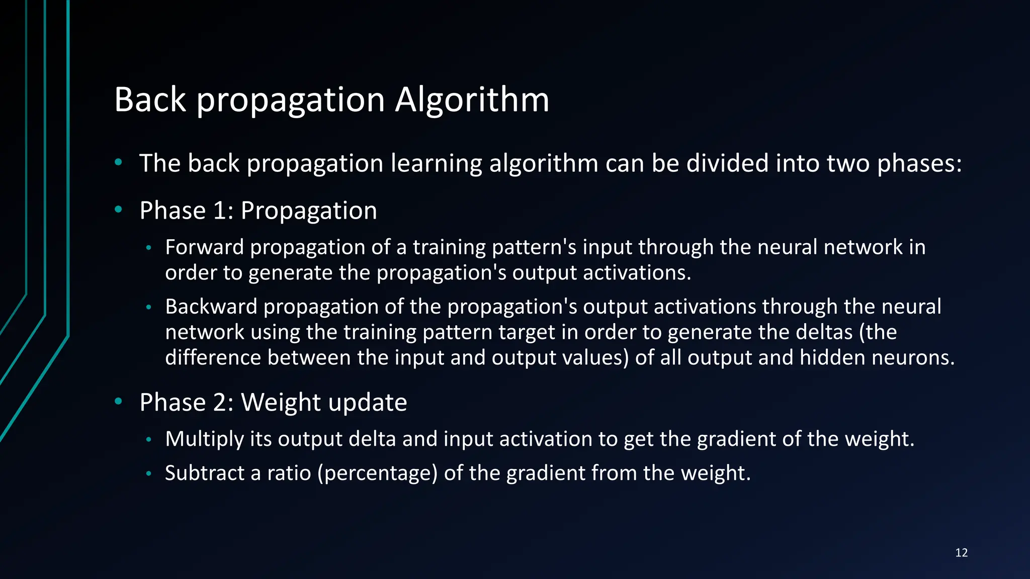
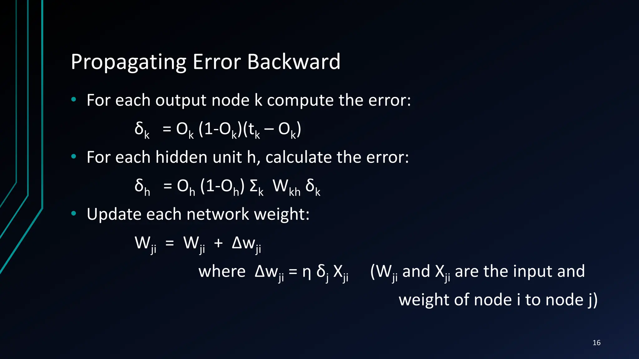
AN INTRODUCTION TO LEARNING INTERNAL
REPRESENTATIONS BY ERROR PROPAGATION
Presented by:
Kunal Parmar
UHID: 1329834
1

2. Outline of the Presentation
• Introduction
• Historical Background
• Perceptron
• Back propagation algorithm
• Limitations and improvements
• Questions and Answers
2

3. Introduction
• Artificial Neural Networks are crude attempts to model the highly
massive parallel and distributed processing we believe takes place in the
brain.
• Back propagation, an abbreviation for "backward propagation of errors",
is a common method of training artificial neural networks used in
conjunction with an optimization method such as gradient descent.
• The method calculates the gradient of a loss function with respect to all
the weights in the network.
• The gradient is fed to the optimization method which in turn uses it to
update the weights, in an attempt to minimize the loss function.
3

4. Why do we need multi layer neural networks??
• Some input and output patterns can be easily learned by single-layer
neural networks (i.e. perceptron). However, these single-layer
perceptron cannot learn some relatively simple patterns, such as those
that are not linearly separable.
• Single layer neural network can’t learn any abstract features of the input
since it is limited to having only one layer. A multi-layered network
overcomes this limitation as it can create internal representations and
learn different features in each layer.
• Each higher layer learns more and more abstract features that can be
used to classify the image. Each layer finds patterns in the layer below it
and it is this ability to create internal representations that are
independent of outside input that gives multi-layered networks their
power.
4

5. Historical Background
• Early attempts to implement artificial neural networks: McCulloch
(Neuroscientist) and Pitts (Logician) (1943)
• Based on simple neurons (MCP neurons)
• Based on logical functions
• Donald Hebb (1949) gave the hypothesis in his thesis “The Organization of
Behavior”:
• “Neural pathways are strengthened every time they are used.”
• Frank Rosenblatt (1958) created the perceptron, an algorithm for
pattern recognition based on a two-layer computer learning
network using simple addition and subtraction .
5
[1]
[1]

6. Historical Background
• However, neural network research stagnated when Minsky and
Papert (1969) criticized the idea of the perceptron discovering two
key issues in neural networks:
• Could not solve the XOR problem.
• Training time grows exponentially with the size of the input.
• Neural network research slowed until computers achieved greater
processing power. Another key advance that came later was
the back propagation algorithm which effectively solved the
exclusive-OR problem (Werbos 1975) .
6
[1]
[1]

7. Perceptron
• It is a step function based on a linear combination of real-valued
inputs. If the combination is above a threshold it outputs a 1,
otherwise it outputs a –1
• A perceptron can only learn examples that are linearly separable.
x1
x2
xn
X0=1
w0
w1
w2
wn
Σ {1 or –1}
7
[3]

8. Delta Rule
• The delta rule is used for calculating the gradient that is used for
updating the weights.
• We will try to minimize the following error:
• E = ½ Σi (ti – oi) 2
• For a new training example X = (x1, x2, …, xn), update each weight
according to this rule:
• wi = wi + Δwi
where, Δwi= -n * E’(w)/wi
8

9. Delta Rule
• The derivative gives,
• E’(w)/wi= Σi (ti – oi)*(- xi)
• So that gives us the following equation:
• ∆ wi = η Σi (ti – oi) xi
9

10. Multi-layer neural networks
• In contrast to perceptrons, multilayer neural networks can not only
learn multiple decision boundaries, but the boundaries may be
nonlinear.
Input nodes
Internal nodes
Output nodes
10
[3]

11. Learning non-linear boundaries
• To make nonlinear partitions on the space we need to define each
unit as a nonlinear function (unlike the perceptron). One solution is
to use the sigmoid (logistic) function. So,
•
• We use the sigmoid function because of the following property,
• d σ(y) / dy = σ(y) (1 – σ(y))
O(x1,x2,…,xn) = σ ( WX )
where: σ ( WX ) = 1 / 1 + e -WX
11
[3]

12. Back propagation Algorithm
• The back propagation learning algorithm can be divided into two phases:
• Phase 1: Propagation
• Forward propagation of a training pattern's input through the neural network in
order to generate the propagation's output activations.
• Backward propagation of the propagation's output activations through the neural
network using the training pattern target in order to generate the deltas (the
difference between the input and output values) of all output and hidden neurons.
• Phase 2: Weight update
• Multiply its output delta and input activation to get the gradient of the weight.
• Subtract a ratio (percentage) of the gradient from the weight.
12

13. Back propagation Algorithm (contd.)
13
[2]

14. What is gradient descent algorithm??
• Back propagation calculates the gradient of the error of the
network regarding the network's modifiable weights.
• This gradient is almost always used in a simple stochastic gradient
descent algorithm to find weights that minimize the error.
w1
w2
E(W)
14
[3]

15. Propagating forward
• Given example X, compute the output of every node until we reach
the output nodes:
Input nodes
Internal nodes
Output nodes
Example X
Compute
sigmoid function
15
[3]

16. Propagating Error Backward
• For each output node k compute the error:
δk = Ok (1-Ok)(tk – Ok)
• For each hidden unit h, calculate the error:
δh = Oh (1-Oh) Σk Wkh δk
• Update each network weight:
Wji = Wji + Δwji
where Δwji = η δj Xji (Wji and Xji are the input and
weight of node i to node j)
16

17. Number of Hidden Units
• The number of hidden units is related to the complexity of the
decision boundary.
• If examples are easy to discriminate few nodes would be enough.
Conversely complex problems require many internal nodes.
• A rule of thumb is to choose roughly m / 10 weights, where m is
the number of training examples.
17

18. Learning Rates
• Different learning rates affect the performance of a neural network
significantly.
• Optimal Learning Rate:
• Leads to the error minimum in one learning step.
18

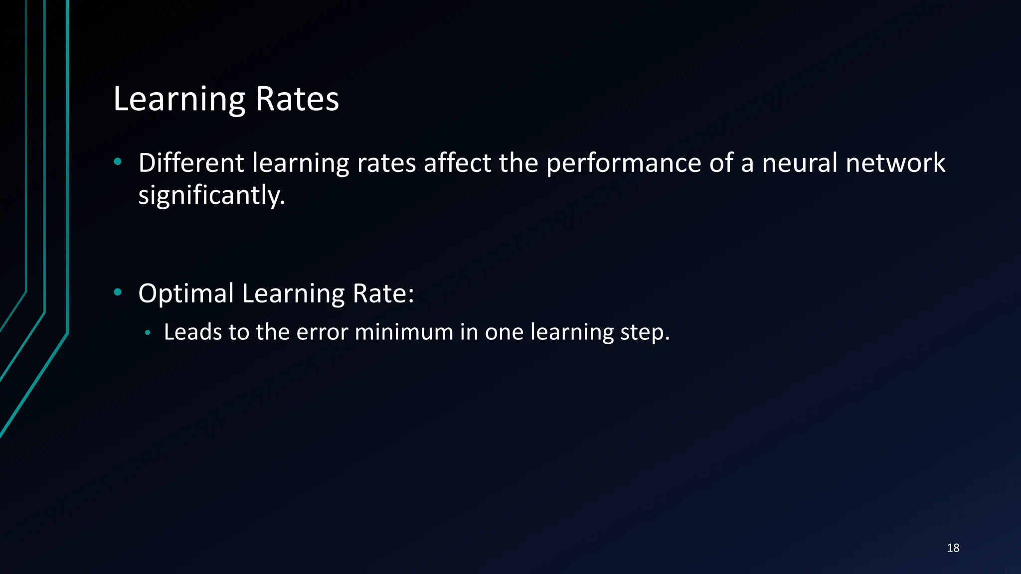
19. Learning Rates
19
[3]

20. Limitations of the back propagation algorithm
• It is not guaranteed to find global minimum of the error function. It
may get trapped in a local minima,
• Improvements,
• Add momentum.
• Use stochastic gradient descent.
• Use different networks with different initial values for the weights.
• Back propagation learning does not require normalization of input
vectors; however, normalization could improve performance.
• Standardize all features previous to training.
20

21. Generalization and Overfitting
• Solutions,
• Use a validation set and stop until the error is small in this set.
• Use 10 fold cross validation
Number of weight updates
Validation set error
Training set error
21
[3]

22. References
• Artificial Neural Networks,
https://en.wikipedia.org/wiki/Artificial_neural_network
• Back propagation Algorithm,
https://en.wikipedia.org/wiki/Backpropagation
• Lecture Slides from Dr. Vilalta’s machine learning class
22

23. Questions??
23

24. Thank you!!
24