OBJECTIVE:-
"Time Series Forecasting Techniques: A Comparative
Analysis"
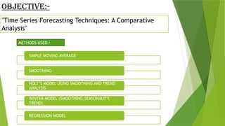
METHODS USED:-
SIMPLE MOVING AVERAGE
SMOOTHING
HOLT’S MODEL USING SMOOTHING AND TREND
ANALYSIS
WINTER MODEL (SMOOTHING,SEASONALITY,
TREND)
REGRESSION MODEL
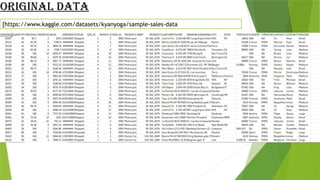
Original data
[https://www.kaggle.com/datasets/kyanyoga/sample-sales-data
DATA CLEANING & PREPROCESSING
Identified and removed any anomalies in the dataset.
Standardized or normalized the data for consistency
Extract the month and year from the "Order Date".
Converted date formats and aggregated data for analysis.
Addressed missing values appropriately for accurate analysis.
Handle any missing or incorrect values
OUTLIER GRAPH
SIMPLE MOVING AVERAGE
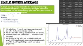
A simple moving average calculates the average price during a
specified period of time. A simple moving average is a technical
indicator that can aid in determining if an asset price will continue or
if it will reverse a bull or bear trend
 We calculate a 12-month moving average to smooth
out sales fluctuations and spot trends.
 We find the index for May 2005 to kick off our forecast
 The forecasted sales for the next 12 months are then
displayed.
 We combine actual sales and forecasted data on a
graph, with actual sales in blue and forecasted sales in
red. This visual helps highlight trends and future
projections.
SMOOTHING MOVING AVERAGE
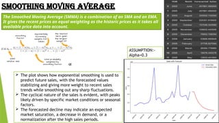
The Smoothed Moving Average (SMMA) is a combination of an SMA and an EMA.
It gives the recent prices an equal weighting as the historic prices as it takes all
available price data into account.
ASSUMPTION:-
Alpha=0.3
 The plot shows how exponential smoothing is used to
predict future sales, with the forecasted values
stabilizing and giving more weight to recent sales
trends while smoothing out any sharp fluctuations.
 The cyclical nature of the sales is evident, with peaks
likely driven by specific market conditions or seasonal
factors.
 The forecasted decline may indicate an expected
market saturation, a decrease in demand, or a
normalization after the high sales periods.
HOLT EXPONENTIAL MODEL WITH TREND
Holt (1957) extended simple exponential smoothing to allow the forecasting
of data with a trend. This method involves a forecast equation and two
smoothing equations (one for the level and one for the trend). Holt's Linear
Trend Method is also called double Exponential Smoothing.
Assumption:-
Alpha = 0.3
Beta = 0.3
 Holt’s exponential smoothing is used with both level (Lt) and
trend (Tt) components, and we initialize them using the sales
value and trend.
 Holt’s Exponential Smoothing not only smoothes the data but
also incorporates a trend component. In this case, the red
forecasted line shows an upward trend, meaning the model
anticipates a positive increase in sales over time.
 The actual sales data shows significant fluctuations and
spikes. Holt’s method aims to capture the trend and smooth
out the noise or volatility
WINTER MODEL ( SMOOTHING, TREND
AND SEASONALITY)
Winter's method assumes that the time series has a level, trend and
seasonal component. A forecast with Winter's exponential
smoothing can be expressed as: The forecast equation is the
extenuation of both the SES and HES methods, finally augmented
with the inclusion of the Seasonal, S, component.
Assumption:-
Alpha=0.3
Beta=0.3
Gamma=0.2
 The actual sales show recurring peaks at regular
intervals, likely pointing to a seasonal component
(e.g., sales spikes due to holidays, promotions, or
other cyclical factors).
 The Winters’ model captures this seasonality, as the
forecast also predicts sharp peaks and valleys at
regular intervals, especially the large spike near
mid-2005 and the subsequent decline, matching the
seasonality seen in the historical data
REGRESSION MODEL
Regression analysis is a set of statistical methods used for the
estimation of relationships between a dependent variable and one or
more independent variables. It can be utilized to assess the strength of
the relationship between variables and for modeling the future
relationship between them.
₹ 0.00 ₹ 200,000.00 ₹ 400,000.00 ₹ 600,000.00 ₹ 800,000.00 ₹ 1,000,000.00₹ 1,200,000.00
0
2000
4000
6000
8000
10000
12000
f(x) = 0.00980465488405837 x + 24.1564326173302
R² = 0.998514407048651
Regression Analysis
Qtyordered Linear (Qtyordered)
Amount
Ordered
Quantity
SUMMARY OUTPUT
Regression Statistics
Multiple R 0.999256927
R Square 0.998514407
Adjusted R Square 0.998459385
Standard Error 8940.774928
Observations 29
 Relation of forecast sales with Qty ordered
 Since adjusted R square close to 1 , so there
is strong correlation between sales and qty
ordered.
 As the amount increases, the ordered
quantity also increases, showing a clear
positive relationship between the two
variables.
 This regression analysis shows a very strong
positive linear relationship between Amount
(in ) and
₹ Ordered Quantity. The data
points closely follow the regression line, and
the R² value of 0.9985 indicates that the
model almost perfectly explains the
relationship between the two variables.
COMPARATIVE ANALYSIS
CONCLUSION
The combined forecast analysis provides a comprehensive view of how different forecasting methods
predict future sales, based on the historical data from 2005.
 Simple Exponential Smoothing (SES): This method assumes a constant level and does not account
for trends or seasonality. The SES forecast shows a smooth prediction, reflecting a basic trend
extrapolated from recent sales data. It is useful for short-term forecasting when the data lacks
significant seasonal patterns or trends.
 Moving Average (MA): By averaging the most recent sales data, the MA forecast provides a smoothed
estimate that can help in understanding the underlying pattern without being overly sensitive to
recent fluctuations. It reflects the average sales trend over the past few months, which is useful for
identifying longer-term trends.
 Holt's Exponential Smoothing: This method extends SES by incorporating a trend component,
allowing it to better capture changes in the growth rate over time. The Holt forecast shows a more
dynamic projection, adapting to changes in the trend, which makes it suitable for data with a clear
upward or downward trend.
 Winters' Exponential Smoothing: This advanced method includes both trend and seasonal
components, offering a detailed forecast that accounts for recurring patterns within the data. The
Winters forecast demonstrates the ability to model complex seasonal effects, providing a more
accurate prediction when seasonality is a significant factor.
THANK YOU.!

SUPPLY CHAIN ANALYTICS, HOLT MODEL WINTER MODEL

  • 1.
    OBJECTIVE:- "Time Series ForecastingTechniques: A Comparative Analysis" METHODS USED:- SIMPLE MOVING AVERAGE SMOOTHING HOLT’S MODEL USING SMOOTHING AND TREND ANALYSIS WINTER MODEL (SMOOTHING,SEASONALITY, TREND) REGRESSION MODEL
  • 2.
  • 3.
    DATA CLEANING &PREPROCESSING Identified and removed any anomalies in the dataset. Standardized or normalized the data for consistency Extract the month and year from the "Order Date". Converted date formats and aggregated data for analysis. Addressed missing values appropriately for accurate analysis. Handle any missing or incorrect values OUTLIER GRAPH
  • 4.
    SIMPLE MOVING AVERAGE Asimple moving average calculates the average price during a specified period of time. A simple moving average is a technical indicator that can aid in determining if an asset price will continue or if it will reverse a bull or bear trend  We calculate a 12-month moving average to smooth out sales fluctuations and spot trends.  We find the index for May 2005 to kick off our forecast  The forecasted sales for the next 12 months are then displayed.  We combine actual sales and forecasted data on a graph, with actual sales in blue and forecasted sales in red. This visual helps highlight trends and future projections.
  • 5.
    SMOOTHING MOVING AVERAGE TheSmoothed Moving Average (SMMA) is a combination of an SMA and an EMA. It gives the recent prices an equal weighting as the historic prices as it takes all available price data into account. ASSUMPTION:- Alpha=0.3  The plot shows how exponential smoothing is used to predict future sales, with the forecasted values stabilizing and giving more weight to recent sales trends while smoothing out any sharp fluctuations.  The cyclical nature of the sales is evident, with peaks likely driven by specific market conditions or seasonal factors.  The forecasted decline may indicate an expected market saturation, a decrease in demand, or a normalization after the high sales periods.
  • 6.
    HOLT EXPONENTIAL MODELWITH TREND Holt (1957) extended simple exponential smoothing to allow the forecasting of data with a trend. This method involves a forecast equation and two smoothing equations (one for the level and one for the trend). Holt's Linear Trend Method is also called double Exponential Smoothing. Assumption:- Alpha = 0.3 Beta = 0.3  Holt’s exponential smoothing is used with both level (Lt) and trend (Tt) components, and we initialize them using the sales value and trend.  Holt’s Exponential Smoothing not only smoothes the data but also incorporates a trend component. In this case, the red forecasted line shows an upward trend, meaning the model anticipates a positive increase in sales over time.  The actual sales data shows significant fluctuations and spikes. Holt’s method aims to capture the trend and smooth out the noise or volatility
  • 7.
    WINTER MODEL (SMOOTHING, TREND AND SEASONALITY) Winter's method assumes that the time series has a level, trend and seasonal component. A forecast with Winter's exponential smoothing can be expressed as: The forecast equation is the extenuation of both the SES and HES methods, finally augmented with the inclusion of the Seasonal, S, component. Assumption:- Alpha=0.3 Beta=0.3 Gamma=0.2  The actual sales show recurring peaks at regular intervals, likely pointing to a seasonal component (e.g., sales spikes due to holidays, promotions, or other cyclical factors).  The Winters’ model captures this seasonality, as the forecast also predicts sharp peaks and valleys at regular intervals, especially the large spike near mid-2005 and the subsequent decline, matching the seasonality seen in the historical data
  • 8.
    REGRESSION MODEL Regression analysisis a set of statistical methods used for the estimation of relationships between a dependent variable and one or more independent variables. It can be utilized to assess the strength of the relationship between variables and for modeling the future relationship between them. ₹ 0.00 ₹ 200,000.00 ₹ 400,000.00 ₹ 600,000.00 ₹ 800,000.00 ₹ 1,000,000.00₹ 1,200,000.00 0 2000 4000 6000 8000 10000 12000 f(x) = 0.00980465488405837 x + 24.1564326173302 R² = 0.998514407048651 Regression Analysis Qtyordered Linear (Qtyordered) Amount Ordered Quantity SUMMARY OUTPUT Regression Statistics Multiple R 0.999256927 R Square 0.998514407 Adjusted R Square 0.998459385 Standard Error 8940.774928 Observations 29  Relation of forecast sales with Qty ordered  Since adjusted R square close to 1 , so there is strong correlation between sales and qty ordered.  As the amount increases, the ordered quantity also increases, showing a clear positive relationship between the two variables.  This regression analysis shows a very strong positive linear relationship between Amount (in ) and ₹ Ordered Quantity. The data points closely follow the regression line, and the R² value of 0.9985 indicates that the model almost perfectly explains the relationship between the two variables.
  • 9.
  • 10.
    CONCLUSION The combined forecastanalysis provides a comprehensive view of how different forecasting methods predict future sales, based on the historical data from 2005.  Simple Exponential Smoothing (SES): This method assumes a constant level and does not account for trends or seasonality. The SES forecast shows a smooth prediction, reflecting a basic trend extrapolated from recent sales data. It is useful for short-term forecasting when the data lacks significant seasonal patterns or trends.  Moving Average (MA): By averaging the most recent sales data, the MA forecast provides a smoothed estimate that can help in understanding the underlying pattern without being overly sensitive to recent fluctuations. It reflects the average sales trend over the past few months, which is useful for identifying longer-term trends.  Holt's Exponential Smoothing: This method extends SES by incorporating a trend component, allowing it to better capture changes in the growth rate over time. The Holt forecast shows a more dynamic projection, adapting to changes in the trend, which makes it suitable for data with a clear upward or downward trend.  Winters' Exponential Smoothing: This advanced method includes both trend and seasonal components, offering a detailed forecast that accounts for recurring patterns within the data. The Winters forecast demonstrates the ability to model complex seasonal effects, providing a more accurate prediction when seasonality is a significant factor.
  • 11.