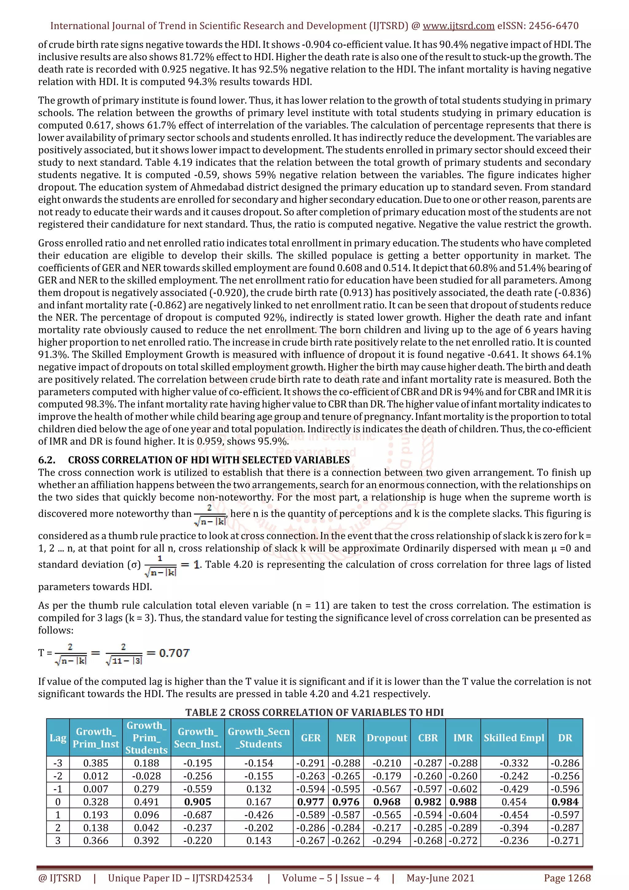
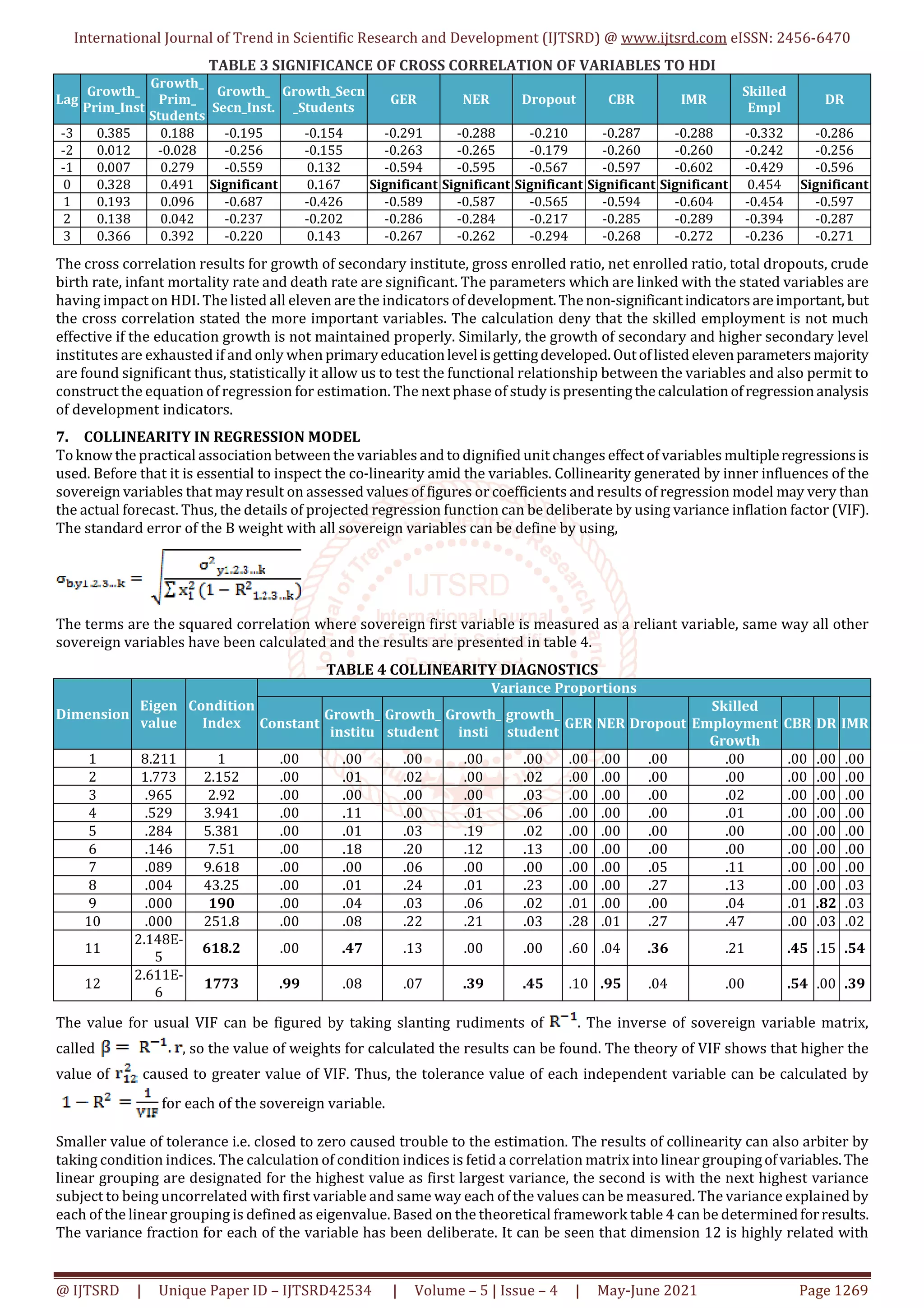
An Application of Multivariate Analysis on Socio Economic Indicators in Gujarat

International Journal of Trend in Scientific Research and Development (IJTSRD)
Volume 5 Issue 4, May-June 2021 Available Online: www.ijtsrd.com e-ISSN: 2456 – 6470
@ IJTSRD | Unique Paper ID – IJTSRD42534 | Volume – 5 | Issue – 4 | May-June 2021 Page 1266
An Application of Multivariate Analysis on
Socio Economic Indicators in Gujarat
Dr. Mahesh Vaghela
Principal and Head of Department of Statistics, N. C. Bodiwala Commerce College, Ahmedabad, Gujarat, India
ABSTRACT
The use of statistical measurement tools to research human behavior in a
social environment is known as social statistics. Statistics and statistical
analysis has become a key feature of social science. In this study researcher
study Socio Economics indicators like Education, Health and Employment in
Gujarat, he also used Multivariate Analysis as a statistical tools. In this
research it will be found that the most of the Sub Indicators are positively
impact on Multivariate Analysis model.
KEYWORDS: Multivariate Analysis, Social sector, Social Indicator, Correlation
How to cite this paper: Dr. Mahesh
Vaghela "An Application of Multivariate
Analysis on Socio Economic Indicators in
Gujarat" Publishedin
International Journal
of Trend in Scientific
Research and
Development(ijtsrd),
ISSN: 2456-6470,
Volume-5 | Issue-4,
June 2021, pp.1266-
1271, URL:
www.ijtsrd.com/papers/ijtsrd42534.pdf
Copyright © 2021 by author (s) and
International Journal ofTrendinScientific
Research and Development Journal. This
is an Open Access article distributed
under the terms of
the Creative
Commons Attribution
License (CC BY 4.0)
(http: //creativecommons.org/licenses/by/4.0)
1. THE CONCEPT OF SOCIAL SECTOR AND SOCIAL
INDICATORS
Social statistics is the use ofstatistical measurementsystems
to study human behavior in a social environment. This can
be accomplished through polling a group of people,
evaluating a subset of data observations and statistical
analysis of a set of data that relates to people and their
behaviors.
Social researcher have used social statistics for many
purposes including
1. The evaluation of the quality of services available to a
group of people.
2. Analyzing behaviors of groups of people in their
environment and special situations.
3. Determining the needs of people through statistical
sampling approach.
Statistics and statistical analysis have become a key feature
of social science. Statistics is of basic importance in all the
behavioral sciences like Economics, Psychology, Political
science, Sociology, Education etc. The use of statistics is so
wide spread in the social sciencethatmanyinstitutessuchas
Harvard also have developed statistical institutes which can
focus on the quantitative aspects of social science. In some
places they havedevelopeddepartmentsofdecisionsciences
for study and research works to be executed in different
disciplines.
2. SOCIAL SECTOR
All social sector statistical activities for collection,
presentation and interpretation of data at central and state
levels are grouped generally under the following categories
of classification. (1) Human Development (2) Education (3)
Health services (4) Women and child Development (5)
Water supply and Sanitation (6) Rural development (7)
Rural Housing (8) Urban development and urban Housing
(9) Employment and training (10) Welfare of weaker
sections (11) Women Welfare (12) Environment (13)
Ecological education etc.
The statistical informationundereachoftheaboveheadsare
collected, compiled and published at state as well as at
central levels. Each of the components in the above list
represents specific situations and corresponding policies
taken by the government and they are clearly mentioned in
the publication year wise.
3. OVERVIEW OF ECONOMY FOR ALL INDIA
GDP at current prices for the year 2012-13 is estimated at
Rs.99.9 Lakh crores and that for 2013-14 is estimated at
Rs.113.5 Lakh crore. This shows a growth of 13.1% and
13.6% during these years. Real GDP (i.e., GDP at constant
prices stands at Rs. 92.8 Lakh crores for 2012-13 and Rs.
99.2 Lakh crores for 2013-14). This shows growth of 5.1%
during 2012-13 and 6.9% during 2014-15isestimatedasRs.
106.57 Lakh crores, showing a growth of 7.4 percent. Per
capita at current prices is Rs. 71,593 andRs.80,388foryears
2012-13 and 2013-14 respectively.Fortheyear2014-15itis
estimated to be Rs.88, 538 thus showing a rise of 10.1% as
compared to previous year. Per capita income at constant
prices (2011-12) is estimated at Rs. 66,344 and Rs. 69,959
for the years 2012-13 and 2013-14 respectively. During the
year 2014-15, it is estimated to be Rs. 74,193 thusshowinga
rise of 6.05% as compared to previous year.
IJTSRD42534

International Journal of Trend in Scientific Research and Development (IJTSRD) @ www.ijtsrd.com eISSN: 2456-6470
4. OVERVIEW OF ECONOMY FOR GUJARAT STATE
Gross state Domestic Product (GSDP) at factor cost at
constant prices in 2013-14 has been estimated at Rs.
4,52,625 crore as against Rs.4,16,163for2012-13showinga
growth of 8.8% GSDP at factor cost atcurrentpricesin2013-
14 has been estimated at Rs. 7,65,638 crores as against Rs.
6,58,540 crores in 2012-13 thus showing a growth of 16.3%
during the year. The share of primary, secondary and
tertiary sectors has been reported as 22.1%, 43.1% and
43.8% respectively to total GSDP in 2013-14 at current
prices. Per capita NSDP at factor cost at constant prices is
estimated at Rs. 63,168 in 2013-14 as against Rs. 59,157 in
2012-13 thus showing a growth of 6.8% during theyear. Per
capita NSDP at factor cost at current prices has been
estimated at Rs. 1,06,831 in 2013-14 as against Rs.93046 in
2012-13 thus showing an increase of 14.8% during theyear.
5. DIFFERENT TYPES OF INDICATORS
Keeping in view the social sector some major indicators can
be listed briefly as under:
1. Human Development Index (HDI) and its ranking (It is
for country wise comparison and the same at state level
SHDI can be helpful for state wise comparison).
2. Education (Quality of Education, Education
Expenditures, Drop out ratios, student/teacher ratio
etc.)
3. Health (Different Health Indicators, Health
Expenditures, Expenses on health to GDP, public health
expenditure to total budget etc.)
4. IMR, MMR, CBR, CDR, Life expectancy at birth etc.
5. Housing (Urban and Rural) (Average household size,
total number of houses, House occupancy, Housing
finance, Affordable housing needs, Employment
6. Water supply and Sanitation etc.
7. Environment etc.
6. CORRELATION AND CROSS CORRELATION
This study is constructed with one important objective that
is to examine the actual impact of HDI and it’s compared
with experts’ opinion. Thus, the study region Ahmedabad
district is selected as study area and for the years 1999 to
2016 (seventeen years) of data for development indicators
and HDI are taken as a secondary data. The data collection
for Education, Health and Employment are taken as an
indicators of development. The education indicators are
growth of primary institutes (Growth Pri_ institu), total
number of students enrolled andgrowthofprimarystudents
(Growth_Pri_student) during the given years, growth of
secondary and higher secondaryinstitute(GrowthSec_insti)
along with growth of total number of students (Growth_Sec
student), general enrollment ratio (GER), net enrollment
ratio (NER) and lastly the dropout (Dropout) from schools
during the given span of time. The second indicator under
study is health. The health indicators are Crude Birth Rate
(CBR), Death Rate (DR) and Infant Mortality Rate (IMR).The
last list of variable is taken as skilled employment in district.
The study of multiple regression is executed for all the listed
parameters. The parameters havebeentestedfordependent
variable Human Development Index (HDI).
6.1. CORRELATION
TABLE 1 CORRELATIONS BETWEEN THE DEVELOPMENT INDICATORS
HDI
Growth
Pri_institu
Growth_Pri_
student
Growth_
Sec_insti
Growth_Sec
student
GER NER Dropout
Skilled
Employment
Growth
CBR DR IMR
HDI 1 -.031 .065 -.363 -.487 -.122 .795 -.775 .366 -.904 -.925 -.943
Growth Pri
_institu
-.031 1 .617 -.068 -.153 -.272 -.123 .039 -.287 .093 .047 .064
Growth_Pri
_student
.065 .617 1 .048 -.590 -.204 .121 -.061 -.382 -.067 .030 -.058
Growth_Sec
_insti
-.363 -.068 .048 1 .209 -.242 -.095 .294 -.221 .209 .349 .257
Growth_Sec
student
-.487 -.153 -.590 .209 1 .062 -.482 .303 .020 .435 .424 .479
GER -.122 -.272 -.204 -.242 .062 1 -.150 .015 .608 .368 .264 .339
NER .795 -.123 .121 -.095 -.482 -.150 1 -.920 .514 .913 -.836 -.862
Dropout -.775 .039 -.061 .294 .303 .015 -.920 1 -.641 .851 .824 .797
Skilled
Employment
Growth
.366 -.287 -.382 -.221 .020 .608 .514 -.641 1 -.310 -.390 -.284
CBR -.904 .093 -.067 .209 .435 .368 .913 .851 -.310 1 .940 .983
DR -.925 .047 .030 .349 .424 .264 -.836 .824 -.390 .940 1 .959
IMR -.943 .064 -.058 .257 .479 .339 -.862 .797 -.284 .983 .959 1
The listed parameters have been tested on basic path. The study of correlation shows the interrelation of the variables. It is
giving an idea about the close impact of variable. It also helps to conclude the inclusive and exclusive impactoftheparameters
on HDI. The standard value for testing is taken 0.5 of r. Those variableshavingatleast 50%impacton eachotherareconcluded.
As it shows higher internal relativity. The bold figures in table 1 shows higher (positive or negative correlation) between the
variables. The net enrollment ratio is positively affect to HDI. It shows 79.5% direct impact. It is clear that higher the enrolled
students get educated and the nation will have learned mass in future. Thus,itiseasiertoemploytheminfuture.Moreover,the
educated population will have faster growth. It shows 63.2%(R2=0.632)inclusiveimpactonHDI.Onotherhandthedropoutis
not a good sign for development. It has negative relation with HDI. It is computed -0.775. It shows 77.5% impactofdropouton
HDI. There are so many reasons for dropout of students from school. It can be measured by taking the determination of r. The
R2 = 0.6006 shows 60.06% dropouts are inclusive reasons and other 39.94% are exclusive reasons for dropoutofthestudents
from school. Higher the birth rate causes higher growth in population. To accommodate the upcoming population in each era
will be the difficult to maintain the economy. The population growth is the major problem for developing countries.Theresult

of crude birth rate signs negative towards the HDI. It shows -0.904 co-efficient value. It has 90.4% negative impact of HDI.The
inclusive results are also shows 81.72% effect to HDI. Higher the death rate is also one oftheresulttostuck-upthegrowth.The
death rate is recorded with 0.925 negative. It has 92.5% negative relation to the HDI. The infant mortality is having negative
relation with HDI. It is computed 94.3% results towards HDI.
The growth of primary institute is found lower. Thus, it has lower relation to the growth of total students studying in primary
schools. The relation between the growths of primary level institute with total students studying in primary education is
computed 0.617, shows 61.7% effect of interrelation of the variables. The calculation of percentage represents that there is
lower availability of primary sector schools and students enrolled. It has indirectly reduce the development. Thevariablesare
positively associated, but it shows lower impact to development. The students enrolled in primary sector should exceed their
study to next standard. Table 4.19 indicates that the relation between the total growth of primary students and secondary
students negative. It is computed -0.59, shows 59% negative relation between the variables. The figure indicates higher
dropout. The education system of Ahmedabad district designed the primary education up to standard seven. From standard
eight onwards the students are enrolled for secondary and highersecondaryeducation.Duetooneorother reason,parentsare
not ready to educate their wards and it causes dropout. So after completion of primary education most of the students are not
registered their candidature for next standard. Thus, the ratio is computed negative. Negative the value restrict the growth.
Gross enrolled ratio and net enrolled ratio indicates total enrollment in primary education. The students who have completed
their education are eligible to develop their skills. The skilled populace is getting a better opportunity in market. The
coefficients of GER and NER towards skilled employment are found 0.608 and 0.514. It depictthat60.8%and51.4% bearingof
GER and NER to the skilled employment. The net enrollment ratio for education have been studied for all parameters. Among
them dropout is negatively associated (-0.920), the crude birth rate (0.913) has positively associated, the death rate (-0.836)
and infant mortality rate (-0.862) are negatively linked to net enrollment ratio. It can be seen that dropout of students reduce
the NER. The percentage of dropout is computed 92%, indirectly is stated lower growth. Higher the death rate and infant
mortality rate obviously caused to reduce the net enrollment. The born children and living up to the age of 6 years having
higher proportion to net enrolled ratio. The increase in crude birth rate positively relate to the net enrolled ratio. It is counted
91.3%. The Skilled Employment Growth is measured with influence of dropout it is found negative -0.641. It shows 64.1%
negative impact of dropouts on total skilled employment growth. Higher the birth may causehigherdeath.The birthanddeath
are positively related. The correlation between crude birth rate to death rate and infant mortality rate is measured. Both the
parameters computed with higher value of co-efficient. It shows the co-efficientofCBR andDR is94%andforCBR andIMR itis
computed 98.3%. The infant mortality rate having higher valuetoCBR thanDR.Thehighervalueofinfantmortality indicatesto
improve the health of mother while child bearing age group and tenure of pregnancy.Infantmortalityistheproportiontototal
children died below the age of one year and total population. Indirectly is indicates the death of children. Thus,theco-efficient
of IMR and DR is found higher. It is 0.959, shows 95.9%.
6.2. CROSS CORRELATION OF HDI WITH SELECTED VARIABLES
The cross connection work is utilized to establish that there is a connection between two given arrangement. To finish up
whether an affiliation happens between the two arrangements, search for an enormous connection, with the relationships on
the two sides that quickly become non-noteworthy. For the most part, a relationship is huge when the supreme worth is
discovered more noteworthy than , here n is the quantity of perceptions and k is the complete slacks. This figuring is
considered as a thumb rule practice to look at cross connection. In the event that the cross relationship of slack k iszerofork =
1, 2 ... n, at that point for all n, cross relationship of slack k will be approximate Ordinarily dispersed with mean μ =0 and
standard deviation (σ) . Table 4.20 is representing the calculation of cross correlation for three lags of listed
parameters towards HDI.
As per the thumb rule calculation total eleven variable (n = 11) are taken to test the cross correlation. The estimation is
compiled for 3 lags (k = 3). Thus, the standard value for testing the significance level of cross correlation can be presented as
follows:
T =
If value of the computed lag is higher than the T value it is significant and if it is lower than the T value the correlation is not
significant towards the HDI. The results are pressed in table 4.20 and 4.21 respectively.
TABLE 2 CROSS CORRELATION OF VARIABLES TO HDI
Lag
Growth_
Prim_Inst
Growth_
Prim_
Students
Growth_
Secn_Inst.
Growth_Secn
_Students
GER NER Dropout CBR IMR Skilled Empl DR
-3 0.385 0.188 -0.195 -0.154 -0.291 -0.288 -0.210 -0.287 -0.288 -0.332 -0.286
-2 0.012 -0.028 -0.256 -0.155 -0.263 -0.265 -0.179 -0.260 -0.260 -0.242 -0.256
-1 0.007 0.279 -0.559 0.132 -0.594 -0.595 -0.567 -0.597 -0.602 -0.429 -0.596
0 0.328 0.491 0.905 0.167 0.977 0.976 0.968 0.982 0.988 0.454 0.984
1 0.193 0.096 -0.687 -0.426 -0.589 -0.587 -0.565 -0.594 -0.604 -0.454 -0.597
2 0.138 0.042 -0.237 -0.202 -0.286 -0.284 -0.217 -0.285 -0.289 -0.394 -0.287
3 0.366 0.392 -0.220 0.143 -0.267 -0.262 -0.294 -0.268 -0.272 -0.236 -0.271

TABLE 3 SIGNIFICANCE OF CROSS CORRELATION OF VARIABLES TO HDI
Lag
Growth_
Prim_Inst
Growth_
Prim_
Students
Growth_
Secn_Inst.
Growth_Secn
_Students
GER NER Dropout CBR IMR
Skilled
Empl
DR
-3 0.385 0.188 -0.195 -0.154 -0.291 -0.288 -0.210 -0.287 -0.288 -0.332 -0.286
-2 0.012 -0.028 -0.256 -0.155 -0.263 -0.265 -0.179 -0.260 -0.260 -0.242 -0.256
-1 0.007 0.279 -0.559 0.132 -0.594 -0.595 -0.567 -0.597 -0.602 -0.429 -0.596
0 0.328 0.491 Significant 0.167 Significant Significant Significant Significant Significant 0.454 Significant
1 0.193 0.096 -0.687 -0.426 -0.589 -0.587 -0.565 -0.594 -0.604 -0.454 -0.597
2 0.138 0.042 -0.237 -0.202 -0.286 -0.284 -0.217 -0.285 -0.289 -0.394 -0.287
3 0.366 0.392 -0.220 0.143 -0.267 -0.262 -0.294 -0.268 -0.272 -0.236 -0.271
The cross correlation results for growth of secondary institute, gross enrolled ratio, net enrolled ratio, total dropouts, crude
birth rate, infant mortality rate and death rate are significant. The parameters which are linked with the stated variables are
having impact on HDI. The listed all eleven are the indicators of development.Thenon-significantindicatorsareimportant, but
the cross correlation stated the more important variables. The calculation deny that the skilled employment is not much
effective if the education growth is not maintained properly. Similarly, the growth of secondary and higher secondary level
institutes are exhausted if and only when primaryeducationlevel isgettingdeveloped. Outoflisted elevenparametersmajority
are found significant thus, statistically it allow us to test the functional relationship between the variables and also permit to
construct the equation of regression for estimation. The next phase of study is presentingthecalculationofregressionanalysis
of development indicators.
7. COLLINEARITY IN REGRESSION MODEL
To know the practical association between the variables and to dignified unit changes effect of variables multipleregressionsis
used. Before that it is essential to inspect the co-linearity amid the variables. Collinearity generated by inner influences of the
sovereign variables that may result on assessed values of figures or coefficients and results of regression model may very than
the actual forecast. Thus, the details of projected regression function can be deliberate by using variance inflation factor (VIF).
The standard error of the B weight with all sovereign variables can be define by using,
The terms are the squared correlation where sovereign first variable is measured as a reliant variable, same way all other
sovereign variables have been calculated and the results are presented in table 4.
TABLE 4 COLLINEARITY DIAGNOSTICS
Dimension
Eigen
value
Condition
Index
Variance Proportions
Constant
Growth_
institu
Growth_
student
Growth_
insti
growth_
student
GER NER Dropout
Skilled
Employment
Growth
CBR DR IMR
1 8.211 1 .00 .00 .00 .00 .00 .00 .00 .00 .00 .00 .00 .00
2 1.773 2.152 .00 .01 .02 .00 .02 .00 .00 .00 .00 .00 .00 .00
3 .965 2.92 .00 .00 .00 .00 .03 .00 .00 .00 .02 .00 .00 .00
4 .529 3.941 .00 .11 .00 .01 .06 .00 .00 .00 .01 .00 .00 .00
5 .284 5.381 .00 .01 .03 .19 .02 .00 .00 .00 .00 .00 .00 .00
6 .146 7.51 .00 .18 .20 .12 .13 .00 .00 .00 .00 .00 .00 .00
7 .089 9.618 .00 .00 .06 .00 .00 .00 .00 .05 .11 .00 .00 .00
8 .004 43.25 .00 .01 .24 .01 .23 .00 .00 .27 .13 .00 .00 .03
9 .000 190 .00 .04 .03 .06 .02 .01 .00 .00 .04 .01 .82 .03
10 .000 251.8 .00 .08 .22 .21 .03 .28 .01 .27 .47 .00 .03 .02
11
2.148E-
5
618.2 .00 .47 .13 .00 .00 .60 .04 .36 .21 .45 .15 .54
12
2.611E-
6
1773 .99 .08 .07 .39 .45 .10 .95 .04 .00 .54 .00 .39
The value for usual VIF can be figured by taking slanting rudiments of . The inverse of sovereign variable matrix,
called , so the value of weights for calculated the results can be found. The theory of VIF shows that higher the
value of caused to greater value of VIF. Thus, the tolerance value of each independent variable can be calculated by
for each of the sovereign variable.
Smaller value of tolerance i.e. closed to zero caused trouble to the estimation. The results of collinearity can also arbiter by
taking condition indices. The calculation of condition indices is fetid a correlation matrix into linear groupingofvariables.The
linear grouping are designated for the highest value as first largest variance, the second is with the next highest variance
subject to being uncorrelated with first variable and same way each of the values can be measured. The variance explained by
each of the linear grouping is defined as eigenvalue. Based on the theoretical framework table 4 can be determinedforresults.
The variance fraction for each of the variable has been deliberate. It can be seen that dimension 12 is highly related with

growth of secondary and higher secondary institutes (39%), growth of the students of secondary and higher secondary
students (45%), Net enrolled ratio (95%), crude birth rate (54%), and infant mortality rate (39%). The condition index
computed 1773 higher for the said variables. Similarly the higher impact is computed for Growth of primary sector institutes
(47%), dropout (36%), crude birth rate (45%) and infant mortality rate (54%). The saidfourindependentvariables arehighly
associated and that may affect the result of regression estimation. The Eigen value is computed most little and the condition
index is recorded with 618.2. The third impacted list of variable is noticed for dimension nine – the death rate has higher
fluctuation of 82% with value of condition index 190. Amid the said sovereign variables, which shows the major influence on
model can be studied by using of tolerance level of variables in table 4.
8. REGRESSION MODEL
Multiple regression is an addition of ordinary least square (OLS). It is used to envisage the value of a variable based on the
value of more than two variables. The variable required to be predict is called the dependentvariableorcriterion variable.The
variables support the value of the reliant variable are called the independent or explanatory variables. It is also help to
determine the explained variance of the model contribution of each of the predictors to it. The first table of concern study is
discussed with model summary, it is given in table 5. It is given the discussionabout R, R2,adj.R2 andtheSEofthe estimate,itis
giving an idea about the model fitting of multiple regression. The R value in model summary table shows 0.984, it is multiple
correlation co-efficient of the model.
TABLE 5 MODEL SUMMARY
R R2 Adj. R2 SE
Change Statistics
Durbin-Watson
R2 Changed F Changed df1 df2 Sig. F Change
.984 .968 .897 .027 .968 13.642 11 5 .005 2.630
R can be considered to be one measure of the value of the estimate of the dependent variable. A value of 0.984 is indicates a
good level of prediction. The R2 column signifies thecoefficientofdetermination, whichistheratioofvarianceinthedependent
variable that can be explained by the independent variables, it is the part of variation taken by the regression model. It can be
seen value of 0.968 that independent variables explain 96.8% of the variability of dependentvariable.Itisalsoinfer intermsof
adjusted R2 to exactly report data.
TABLE 6 ANOVA
Model SS df MSS F Sig.
Regression .108 11 .010 13.642 .005
Residual .004 5 .001
Total .112 16
The F-statistics – analysis of variance is studies whether the overall regression model is a good fit for thedata ornot.Thetable
6 shows that the independent variables statistically predict the dependent variable, F (11, 5) = 13.64, p < 0.005 - i.e., the
regression model is a good fit of the data.
Following is the table of regression co-efficient relate to the dependent variable HDI. There are total elvenvariables affectsthe
HDI. The individual effect of each of the variable is presented in table 6. The constant of the model is found positive. Thus,
negative the value of independent variable reduce the constant and positive the value of coefficient increase the value of
constant. The basic multivariable model can be rewrite as follows:
The simple multiple regression models can be determined as:
Thus we may finally write the multiple regression models as:
TABLE 7 COEFFICIENTS
Unstand Coeff. Stand.Coeff.
t Sig.
95.0% Confi. Interval for B Collinearity Statistics
B SE Beta Lower Bound Upper Bound Tolerance VIF
Const. 2.516 3.043 .827 .446 -5.305 10.34
Growth_institu .011 .008 .266 1.359 .232 -.010 .032 .168 5.948
Growth_student .004 .008 .152 .572 .592 -.025 .016 .091 10.97
Growth_insti .004 .005 .112 .720 .504 -.009 .016 .265 3.780
growth_student .001 .004 .061 .269 .799 .011 .009 .127 7.868
GER .017 .008 .718 2.231 .076 -.003 .036 .062 16.05
NER .017 .025 .389 .693 .519 -.081 .046 .021 48.77
Dropout -.001 .003 -.135 -.288 .785 -.007 .009 .029 34.21
Skilled Empl. Growth .005 .005 .328 .988 .368 .017 .008 .058 17.09
CBR -.078 .072 -1.630 -1.08 .330 -.264 .108 .003 354.3
DR -.054 .062 -.348 -.874 .422 -.212 .104 .041 24.57
IMR -.002 .010 -.188 -.159 .880 -.023 .026 .005 216.2

The depicted model can be rewrite as:
CONCLUSION:
The study of correlation is discussed to understand the
direct relation betweenthevariables.Statistically,theresults
are interrelated and sometimes the variable is associated
with itself.
Table 7 shows the final presentation of multiple regression
model. This model is defined for listed 11 independent
variables relate to development anddependentvariable HDI
of Ahmedabad district for the year 1999 to 2017. The model
is presented with constant of the model, standard values of
co-efficient (beta), unstandardized co-efficient B, t statistics
and standards of collinearity. The lower value of tolerance
are computed for growth of primary student (0.091), GER
(0.062) NER (0.021), Dropout (0.029),SkilledEmployment
Growth (0.058), CBR (0.003), DR (0.041) and IMR (0.005).
Lower the value of tolerance indicates best fit of the model.
The concluded results of model can be interpreted as
follows:
The growth of primary institute (0.011) having positive
impact on constant. It shows that increase in primary
institute will result higher in development of education. As
the total primary institute have positive impact on model
indirectly the growth of total number of students will
increase. It shows that the growth of primary students have
increased 0.004 to HDI. Similarly, the growth of secondary
institute and total number of secondary and higher
secondary have positive impact on model. The growth of
secondary and higher secondary level institute increases as
0.004 and for total number students’ growth it is computed
0.001. Two other variablerelatingtoeducationdevelopment
are found positive towards the constant of HDI. GER (0.017)
and NER (0.017) both the parameters showsequal impactto
the constant. All the parameters of education have positive
impact to development of HDI. It is advisable to focus more
to increase the education related parameters to have
increase in HDI. The only parameter of education is
computed negative i.e. dropout of students. It clearly stated
that higher the dropout reduce the HDI. The officials should
design proper strategy to reduce total dropouts. The skilled
employment growth is also have positive association
towards the constant of model. It shows 0.005 value in
increment of HDI. Health wise the district officials required
to do more improvement majority of the indicators have
negative sign towards the constant is shows reduction of
HDI. Reduction in CBR is computed 0.078, the co-efficient of
death rate is 0.054 and for infant mortality it is recorded
0.002. All the three health related indicators are computed
negative with higher value of co-efficient.
REFERENCES:
[1] Abhishek T. (1992).ImplicationabouttheVariablesof
a Factor model with changing alteration. Metrical 36-
49.
[2] Abusaleh Shariff (1995) health Transition in india,
NCAER, Oct 1995
[3] Adnan (1984) Approximation of OLS based on robust
testing. Math-Statistics, 67-85.
[4] Bagchi, K.K. (2011). Regional Disparities in India’s
Socio-economic Development. New Century
Publications. New Delhi. India 6)
[5] Bajpai, N, Sachs, J.D. (1996). Trends in Inter-State
Inequalities of Income in India. Development
Discussion Paper No. 528. Harvard Institute for
International Development, Harvard University.
[6] BRICS (2012). Joint Statistical Report, 2012, BRICS.
[7] Bunge, M. (1981). Development Indicators. Social
Indicators Research, 9(3), 369- 385. 11)
[8] Carr-Hill, R. (2013). Missing Millions and Measuring
Development Progress. World Development, 46, 30–
44. 29
[9] Cetaler, S. Miranda (1997): Principle Component
Analysis, NY, Alabama.
[10] Dubey, A. (2009). Intra-State Disparities in Gujarat,
Haryana, Kerala, Orissa and Punjab. Economic and
Political Weekly, 44(26&27), 224–230.
[11] Dutta, S. (2011). Efficiency in Human Development
Achievement: A Study of Indian States. Margin: The
Journal of AppliedEconomic Research,5(4),421–450.
[12] Grene William (2003),EconometricAnalysis,Prentice
Hall New York.
[13] Harris, R. J.: A Primer of Multivariate Statistics. New
York, Academic Press, 1975.
[14] Huberty, C. J., and J. D. Morris. 1989. Multivariate
analysis versus multiple univariate
analyses. Psychological Bulletin 105:302–308.
[15] International Encyclopedia of the Social Sciences
[16] Jha, R. (2014). Welfare Schemes and Social Protection
in India. International Journal of Sociology and Social
Policy, 34(3/4), 214–231.
[17] Luc Anselin, Sheri Hudak, Spatial econometrics in
practice A review of software options, September
1992, Regional Science and Urban Economics
[18] Lutz, M. (1988). On Criteria of Socioeconomic
Development. Paper presented at the annual meeting
of the Allied Social Science Associations, New York,
1988.
[19] Myrdal, G. (1972). Asian Drama: An Inquiry into the
Poverty of Nations. Vintage Book, New York.
[20] Nagaraj R.A., Varoudakis, A., Veganzones, M. (1998).
Long-Run Growth Trends and Convergence across
Indian States. Working Paper No. 131. OECD
Development Centre.
[21] Rakesh Shrivastava (2011) Statistical Evaluation of
socioeconomic development some recent technique.
Sankhyavignan NSV 7, No.1 & 2
[22] Raymond J.G.M. Florax, Vrije Universities Amsterdam
and University of Amsterdam; Peter Nijkamp, Vrije
Universities Amsterdam, Misspecification in Linear
Spatial Regression, Models, 2004
[23] Sanjay G. Raval And Mahesh H. Vaghela (2016), “Brief
Review for Quality of Education In Institutions of
Gujarat State”, presented in Quest for Excellence and
Efficiency in Higher Education, organized by H. L.
Commerce College and A. G. Teachers College, 30th
Sept – 1st Oct. – 2016.

An Application of Multivariate Analysis on Socio Economic Indicators in Gujarat

More Related Content

What's hot

Similar to An Application of Multivariate Analysis on Socio Economic Indicators in Gujarat

More from ijtsrd

Recently uploaded

An Application of Multivariate Analysis on Socio Economic Indicators in Gujarat