Download to read offline


![1-4 MATHEMATICS
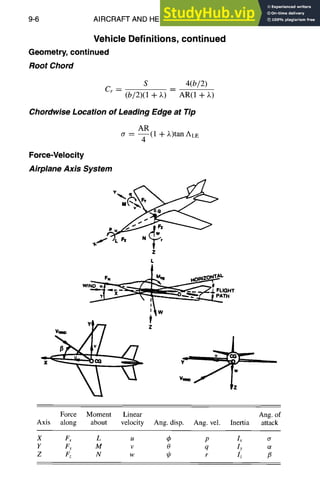
Algebra, continued
Logarithms
{_+~ whenb lies between O and l
logb b = t, logb 1 = 0, logb 0 = when b lies between 1 and cx~
logb M • N = logb M + logb N
logb N p = p logb N
logb N -- l°ga N
log~ b
M
logb ~- = log~ M - logb N
10gb ~ = t7 logb N
r
logb b N = N blOgb
N = N
The Quadratic Equation
If
then
ax 2 +bx + c = 0
-b 4- ~/~ - 4ac 2c
X ~
2a -b q: ~ - 4ac
The second equation serves best when the two values of x are nearly equal.
> | the roots are real and unequal
If b2 - 4ac = 0 / the roots are real and equal
< the roots are imaginary
The Cubic Equations
Any cubic equation y3 + py2 -t- qy + r = 0 may be reduced to the form x 3 +
ax + b = 0 by substituting for y the value [x - (p/3)]. Here a = 1/3(3q - p2),
b = 1/27(2p 3 - 9pq + 27r).
Algebraic Solution ofx 3 + ax + b = 0
If
f b ~ a 3
A= -~+ +2-7
f b ~/~ a3
B= -~- + 2--7
x =A+B
A+B A-B A+B A-B l-Z-
~
+--5--4=3 2
b2 a 3 > / 1 real root, 2 conjugate imaginary roots
- - = 0 / 3 real roots, at least 2 equal
4 + ~ < 3 real and unequal roots](https://image.slidesharecdn.com/aiaaaerospacedesignengineersguide-230807164453-d76eba30/85/Aiaa-Aerospace-Design-Engineers-Guide-pdf-13-320.jpg)
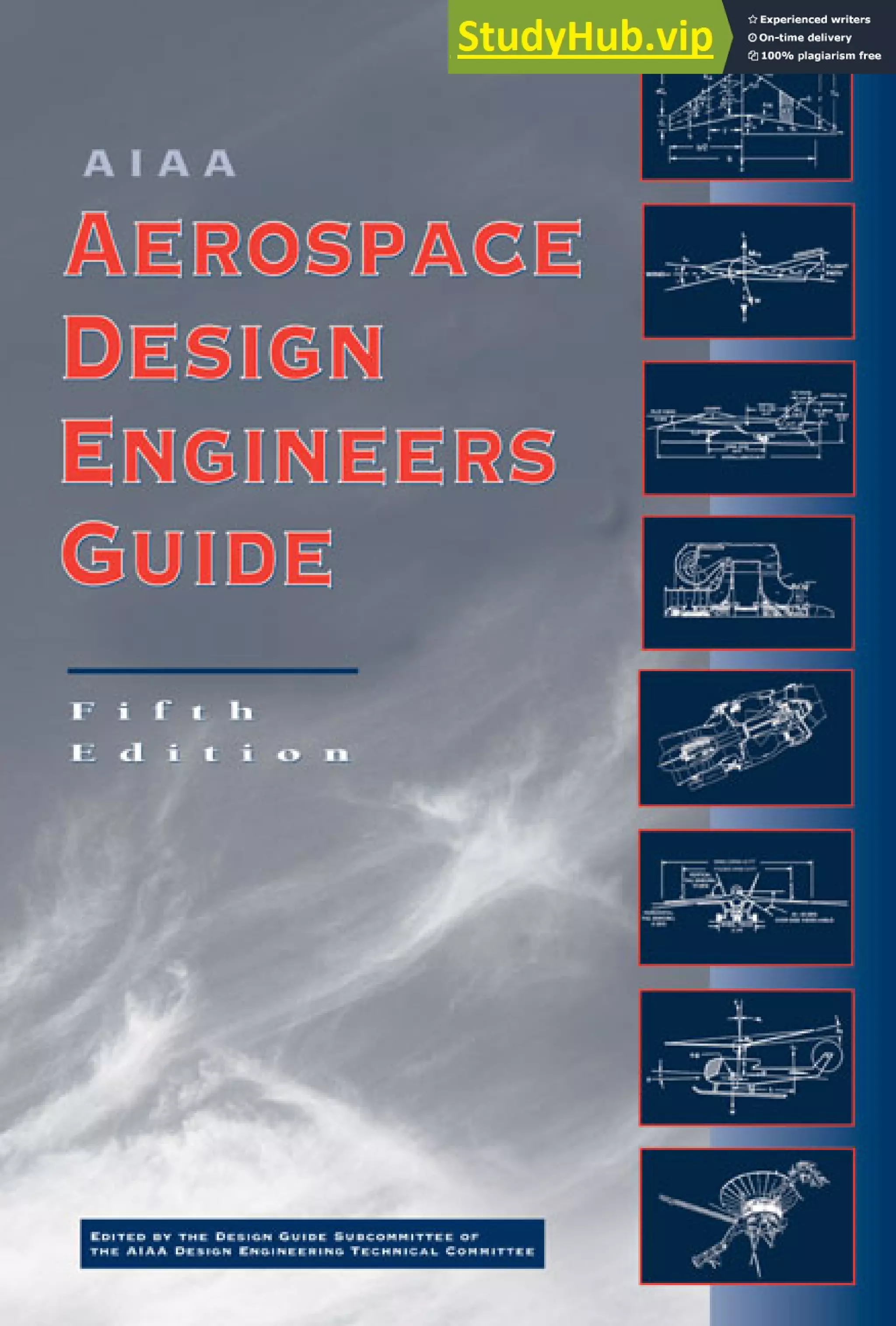
![MATHEMATICS 1-5
Algebra, continued
Trigonometric Solution for x 3 + ax + b = 0
Where (b2/4) + (a3/27) < 0, these formulas give the roots in impractical form
for numerical computation. (In this case, a is negative.) Compute the value of angle
4~derived from
ta )
cosy = + -~
x = q:2 3 cos 3
Then
where the upper or lower signs describe b as positive or negative.
Where (b2/4) + (a3/27) >= 0, compute the values of the angles ~ and q~from
cot 2~p = [(b2/4) + (a 3/27)] 1/2, tan 4>= (tan ~) 1/3. The real root of the equation
then becomes
x = +2 cot 2~b
where the upper or lower sign describes b as positive or negative.
When (b2/4) + (a3/27) = 0, the roots become
x = T2 3 3
where the upper or lower signs describe b as positive or negative.
The Binomial Equation
When x n = a, the n roots of this equation become
a positive:
Q'a( 2kJr 2kzr)
x = cos + ~ sin
n n
a negative:
~/~-d [ (2k + 1)7r (2k + 1)re]
x = cos + -v/-S1 sin --
n Y/
where k takes in succession values of 0, 1, 2, 3..... n - 1.](https://image.slidesharecdn.com/aiaaaerospacedesignengineersguide-230807164453-d76eba30/85/Aiaa-Aerospace-Design-Engineers-Guide-pdf-14-320.jpg)
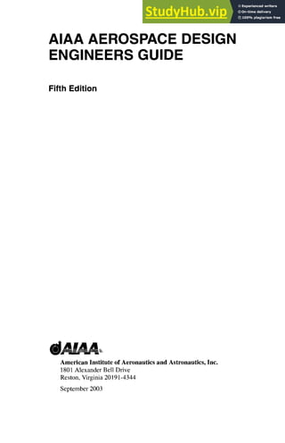
![Note: A ---- area, V = volume
ObliqueTriangleSolution
Right Triangle
I
A= 2ab
a = ~v/-~-b 2
MATHEMATICS
Mensuration
C= V/-~a
2 q- b2
b=q~-a 2
Oblique Triangle
A = ½bh
Equilateral Triangle
A= ½ah=Ja2,v/3
h---- ½av/3
a
rl -- 2v/~
a
Parallelogram
A ----ah = ab sinot
d] = ~/a2 + b2 - 2 ab cos et
d2 = ~/a2 + b2 + 2 ab cos ot
Trapezoid
I h(a + b)
A=~
1-9
I"!1"......... a -°°--°°~,1
I,,~°H°o°°° °b ....... D,, I
"~,
4 °,~,
o°~ ....... .. ,,
.... ,/ i
v',,B"....... a .......
~-..b--4](https://image.slidesharecdn.com/aiaaaerospacedesignengineersguide-230807164453-d76eba30/85/Aiaa-Aerospace-Design-Engineers-Guide-pdf-18-320.jpg)
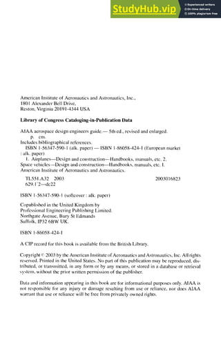
![MATHEMATICS 1-11
Mensuration, continued
Area by Approximation
If Y0, Yl, Y2, ..., y. are the lengths of a series of
equally spaced parallel chords and if h is their dis-
tance apart, the area enclosed by boundary is given
approximately by i i I |
~l, I', , L.."
As = ih[(yo + Yn)+ 4(yl + Y3 -'1-"'" -}-y.-~) + 2(y2 + Y4 -I- "'" -I- Yn-1)]
where n is even (Simpson's Rule).
Ellipse
A = zrab/4
Perimeter s
__7r(a+b) [ 1 (a-b]2+ 1 (a-b~ 1 (a-b] 6 ]
4 a+b.] ~ a+b] +~ ~a+b/ +""
(a+b) 3(1 +X) +
~rr 8 ~
?
where X = L2(a + b) J
Parabola
Length of arc s
A = (2/3)1d
1 2 12 [4d+~/16d2+12)
= ~/16d q- 12 --~ ~-'~~,~t l
=1 1+3 1 / -5
d
Height of segment dl = ~(12 _ l2)
v/-d- dl
Width of segment 11 = l -~](https://image.slidesharecdn.com/aiaaaerospacedesignengineersguide-230807164453-d76eba30/85/Aiaa-Aerospace-Design-Engineers-Guide-pdf-20-320.jpg)
![MATHEMATICS 1-13
AnalyticGeometry
Rectangular and Polar Coordinate Relations
x = r cos0 y = r sin0
r = ~5 + yZ 0 = tan -J y sin0 -- Y
x ~r~+y 2
x y
cos 0 -- tan 0 ------
~ y 2 x
Points and Slopes
For P1 (x l, Yl) and P2(x2, Y2) as any two points and ~ the angle from OX to P1 P2
measured counterclockwise,
P1P2 = d = v/(x2 -Xl) 2 + (22 -- 21) 2
xl + x2 Yl + Y2
P1 P2 midpoint -- 2 ' 2
For point m2 that divides PI P2 in the ratio m 1,
m]x2 + m2x, mlY2 + m2Yl ~
ml -}- m2 ' ml + m2 /
Y2 - Yl
Slope of P1 P2 = tan a = m -
X2 -- X1
For angle/3 between two lines of slopes ml and m2,
/3 = tan -1 m2 - - ml
1 + mlm2
P1
J o
Y
P2
Straight Line
Ax+By+C =0
-A -- B = slope
y=mx+b
(where m = slope, b = intercept on OY)
y - Yl = m(x-x~)
O
Y ;2(x2,Y2)
d
XI
[m= slope, where P](Xl, Yl) is a known point on line]
Ax2 + By2 + C
d=
-]-~A'-f + 9 2
[where d equals distance from a point Pz(x2, Y2) to the line Ax + By + C = 0]](https://image.slidesharecdn.com/aiaaaerospacedesignengineersguide-230807164453-d76eba30/85/Aiaa-Aerospace-Design-Engineers-Guide-pdf-22-320.jpg)
![MATHEMATICS
Analytic Geometry, continued
Parabola
Conic where e = 1; latus rectum, a = LR.
Parabola A
Y
(y - k) 2 = a(x - h) Vertex (h, k), axis I] OX
y2 = ax Vertex (0, 0), axis along OX
1-15
vi
h,
x
Parabola B
(x-h) 2 =a(y-k) Vertex(h,k), axis II OY
X 2 = ay Vertex (0, 0), axis along OY ii
/
1
Distance from vertex V to focus F: ~ a
A
Y V(h,k)
Sine Wave
y = a sin(bx + c)
y = a cos(bx + c') = a sin(bx + c) (where c = c' + Jr/2)
y = m sin bx + n cos bx = a sin(bx + c)
(where a = ~m 2 + n 2, c = tan -x n/m)
Y](https://image.slidesharecdn.com/aiaaaerospacedesignengineersguide-230807164453-d76eba30/85/Aiaa-Aerospace-Design-Engineers-Guide-pdf-24-320.jpg)
![1-16 MATHEMATICS
Analytic Geometry,continued
Exponential or Logarithmic Curves
l) y = ab x orx = logb y ".,(2)
a
2) y = ab -x or x = - logb ya : ""
"o
3) x=abYory=tog h-
a 0
X
4) x = ab -y or y = - logb -
a
The equations y = ae ±"x and x = ae ±ny are special cases.
(1) (3)
%...._ X
I -"........ (4)
Catenary
Line of uniform weight suspended freely between two points at the same level:
y= a[cosh(X) - 1]= a(ex/a2"+e-X/a-2a)
(where y is measured from the lowest point of the line, w is the weight per unit
length of the line, Th is the horizontal component of the tension in the line, and a
is the parameter of the catenary; a = Th/W)
Helix
Curve generated by a point moving on a cylinder with the distance it transverses
parallel to the axis of the cylinder being proportional to the angle of rotation about
the axis:
x = acosO
= a sin 0
Y
......."-"..' I
z =kO
,'"...... 2~'kl
(where a = radius of cylinder, 2zrk -=--pitch) .,~ .... 2,1](https://image.slidesharecdn.com/aiaaaerospacedesignengineersguide-230807164453-d76eba30/85/Aiaa-Aerospace-Design-Engineers-Guide-pdf-25-320.jpg)
![MATHEMATICS 1-17
Analytic Geometry, continued
Points, Lines, and Planes
Distance between points P~(xl, Yl, Zl) and P2(x2, Y2, Z2):
d = ~/(x 2 - Xl) 2 --~ (Y2 - Yl) 2 + (z2 - Zl) 2
Direction cosine of a line (cosines of the angles t~,/3, y which the line or any
parallel line makes with the coordinate axes) is related by
cosz ot + cos2/3 + cos2 y = 1
If cosa:cos/3:cosy=a:b:c, then
a b
COS (~ ~ COS/3
~/a 2 + b 2 + c 2 ~/a 2 q- b 2 + c 2
c
COS y
~/a 2 + b 2 + c 2
Direction cosine of the line joining P1(Xl, y~, zl) and P2(x2, Y2, Z2):
COSCt : COS/3 : COSy = X2 -- Xl : Y2 -- Y~ : Z2 -- Zl
Angle 0 between two lines, whose direction angles are cq,/31, Y1 and ot2,/3z, Y2:
COS 0 = COS ffl COS Ol2 -~- COS/31 COS/32 -]- COS YI COS Y2
Equation of a plane is of the first degree in x, y, and z:
Ax + By + Cz + D = 0
where A, B, C are proportional to the direction cosines of a normal or perpendi-
cular to the plane.
Angle between two planes is the angle between their normals. Equations of a
straight line are two equations of the first degree.
Alx + Bly + ClZ + D1 = 0 A2x + B2y + C2z + D2 = 0
Equations of a straight line through the point PI (x l, Yl, z l) with direction cosines
proportional to a, b, and c:
x - Xl Y - Yl z - Zl
a b c
Differential Calculus
Derivative Relations
dy dx
Ifx = f(y), then ~- = 1 + dy
dy dy dx
If x = f(t) and y = F(t), then -- +
dx dt dt
If y = f(u) and u = F(x), then dy = dy du
dx du dx](https://image.slidesharecdn.com/aiaaaerospacedesignengineersguide-230807164453-d76eba30/85/Aiaa-Aerospace-Design-Engineers-Guide-pdf-26-320.jpg)
![1-18 MATHEMATICS
Differential Calculus, continued
Derivatives
Functions of x represented by u and v, constants by a, n, and e:
~(x) = 1 (a) = 0
d du dv
d du d aU = a.~adU
~(au) = ad~ ~ dx
d dv du
= +
du _ u~
d = v~
d_____(u.) = n-1 du
nu -~
d
loga u -
d
dx
d du d du
-- cos u = -sin u-- -- tan u = see 2 u
dx dx dx dx
d d 1 du
-- cot u = -csc 2 u du -- sin-1 u -- - -
dx dx dx ~/1 - - U2 dx
(where sin -l u lies between -rr/2 and +rr/2)
d 1 du
-- COS -1 U --
dx ~/]- -- u2 dx
(where cos -1 u lies between 0 and Jr)
1 du d 1 du
d tan- 1 u -- -- cot -1 u --
dx 1 +u2dx dx
_ 1 du
d sec l u-
dx uw/~-- 1 dx
(where sec -1 u lies between 0 and zr)
d 1 du
-- csc -1 U
dx uv~-- I dx
(where csc -1 u lies between -re/2 and +re/2)
d du
--e u = e u-
dx dx
d uV vuV_ 1 du v dv
= + u
d du
-- sin u = cos u --
dx dx
log a e du
u dx
1 du
udx
1 +u2dx](https://image.slidesharecdn.com/aiaaaerospacedesignengineersguide-230807164453-d76eba30/85/Aiaa-Aerospace-Design-Engineers-Guide-pdf-27-320.jpg)
![1-22 MATHEMATICS
Differential Equations
Equations of First Order and First Degree: Mdx + Ndy = 0
Variables Separable
XIY] dx + X2Y2 dy = 0
X1 dx Y2 dy
Homogeneous EquaHon
f
[dv/f(v)-vl y
x = Ce and v = -
x
M -- N can be written so that x and y occur only as y -- x, if every term in M and
N have the same degree in x and y.
Linear Equation
dy + (Xly - X2)dx = 0
y=e-fx, e~(fX2efX'e'Xdx+C)
A similar solution exists for dx + (Ylx - Y2) dy = 0.
Exact Equation
Mdx + Ndy = 0 where OM/Oy = ON/Ox
O
fMx+f
for y constant when integrating with respect to x.
Nonexact Equation
Mdx + Ndy = 0 where OM/Oy # ON/Ox
Make equation exact by multiplying by an integrating factor /*(x, y)--a form
readily recognized in many cases.](https://image.slidesharecdn.com/aiaaaerospacedesignengineersguide-230807164453-d76eba30/85/Aiaa-Aerospace-Design-Engineers-Guide-pdf-31-320.jpg)
![MATHEMATICS 1-23
Complex Quantities
Properties of Complex Quantities
If z, Zl, z2 represent complex quantities, then
Sum or difference: Zl 4- Z2 = (Xl -{-X2) "~ j(y~ ± Y2)
Product: zl • Z2 = rlr2[cos(01 + 02) ± j sin(01 + 02)]
= rlr2 ej(O'+02) = (XlX2 -- YlY2) ± j(xlY2 Jr-x2Yl)
Quotient : zl/z2 = rl/rz[cos(01 - 02) + j sin(0~ - 02)]
• x2yl - - Xl Y2
_~ rleJ(O~_o2 ) _ XlX2 4- YlY2 + J y2
r2 + + 2
Power: z n = r n [cos nO + j sin nO] = rne jn°
0 + 2krr 0 + 2krr = ~/~ej(O+2krc/n)
Root: ~ = ~/r cos - - + j sin - -
n n
where k takes in succession the values 0, 1, 2, 3 ..... n - 1.
If zl = z2, then x~ = x2 and y~ = Y2.
Periodicity: z = r(cos 0 + j sin 0)
= r[cos(0 + 2kzr) + j sin(0 + 2kzr)]
or
Z = re j° ~ re j(O+2kzr) and e i2k~r = 1
where k is any integer.
Exponential-trigonometric relations:
e jz = cos z ± j sin z e -jz = cos z - j sin z
1 1 . _ e_jZ )
cos z = -~(e jz + e -jz) sin z = (e lz
z
Some Standard Series
Binomial Series
n(n -- 1)an_2x 2
(a + x) n = a n 4- na n - ix + - -
2!
n(n -- 1)(n -- 2)a n_3x 3 + (x 2 < a2 )
-JI- • • •
3~
The number of terms becomes infinite when n is negative or fractional.
( bx b2x2 b3x 3 )
(a - bx) -1 = i 1 ± -- + + +.-- (b2x 2 < a 2)
a a -7](https://image.slidesharecdn.com/aiaaaerospacedesignengineersguide-230807164453-d76eba30/85/Aiaa-Aerospace-Design-Engineers-Guide-pdf-32-320.jpg)
![1-24 MATHEMATICS
Some Standard Series, continued
Exponential Series
(X f~,~a)2 (x~a) 3
ax = l + x ~ a + - + - + . . .
2! 3!
x 2 x 3
eX=l+x+~.. +~. + "'"
Logarithmic Series
fi, X = (X -- 1) -- l(x -- 1) 2 + l(x -- 1) 3 .... (0 < X < 2)
x-1 1 (X 1) 2 1 (X I) 3 ( ~ )
+ + x +
Ix-1 1 (x-l~ 3 1 (x-l~ 5 1
Cx = 2 ~-~. ~ x + 1] + 5 x--~] +"" (x positive)
x 2 x 3 x 4
f.(1 +x) = x - T + T - -4-
+...
Trigonometric Series
X 3 X 5 X 7
sin x = x - ~.T + 5~- - 7-~ +'
X 2 X 4 X 6
cosx = 1 - -- + -- - -- +
2! 4! 6!
x3 2xS17x7 62x9 ( ~--~-4
)
tanx=x+~-+~-+ 3--i-~-+2--~-~+... x2<
lx 3 1 .3x 5 1 .3-5x 7
sin-lx=x+7~-+2~523.4 +2.4-~7 +'" (x2<l)
1 1 1
tan-l x=x--x 3+_x 5--x 7+... (x2<1)
3 ~ 7 =](https://image.slidesharecdn.com/aiaaaerospacedesignengineersguide-230807164453-d76eba30/85/Aiaa-Aerospace-Design-Engineers-Guide-pdf-33-320.jpg)
![1-26 MATHEMATICS
Matrix Operations, continued
In general, matrix multiplication is not commutative: AB # BA. Matrix multi-
plication is associative: A(BC) = (AB)C. The distributive law for multiplication
and addition holds as in the case of scalars.
(A + B)C = AC + BC
C(A + B) = CA + CB
For some applications, the term-by-term product of two matrices A and B of
identical order is defined as C = A • B, where cij = aijbij.
(ABC)' = C' B' A'
(ABC) H = CHBHAH
If both A and B are symmetric, then (AB)' = BA. The product of two symmetric
matrices will usually not be symmetric.
Determinants
A determinant IAI or det(A) is a scalar function of a square matrix.
IAIIBI = lAB{
IA I = all a12 =alla22--a12a21
a21 a22
IAI = IA't
a12 a13
]A] = ;;11 a22 a23 =alla22a33 +a12a23a31 +a13a21a32
O31 032 033 --a13022031 -- alla23a32 -- a12a21a33
all a12 • • • aln
fAI = a21
. . . . .
a22 '" a2n = Z (_l)~ali,a2 i ..... anin
lanl an2 • • • anm r
where the sum is over all permutations: il # i2 # '" # in, and 3 denotes the
number of exchanges necessary to bring the sequence (il, i2..... in) back into the
natural order (1, 2 ..... n).](https://image.slidesharecdn.com/aiaaaerospacedesignengineersguide-230807164453-d76eba30/85/Aiaa-Aerospace-Design-Engineers-Guide-pdf-35-320.jpg)
![MATHEMATICS 1-27
Curve Fitting
Polynomial Function
y = bo + blx + b2x2 Jr- • • • -[- bmxm
For a polynomial function fit by the method of least squares, obtain the values of
bo, bl ..... bm by solving the system of m + 1 normal equations.
nbo + blEXi + b2Ex2i + ... + bm~x m = ~Yi
b~]xi + blEx~ + b2Ex 3 +"" + bmExm+l = ~]xiYi
boEx m + bl]~Xm+l ~- b2~x m+2 +... q- bm~x 2m ~_ ~x?y i
Straight Line
y --- bo --I-blX
For a straight line fit by the method of least squares, obtain the values b0 and bl
by solving the normal equations.
nbo + bl EXi = Eyi
bo~xi q-bl~x 2 = ]~xiYi
Solutions for these normal equations:
n~xiYi - - (]~Xi)(~yi) ~Yi ~Xi
bl = nEx2i _ (]~xi)2 b0 -- n bl--n = ~ - blX
Exponential Curve
y =ab x or logy----loga+(logb)x
For an exponential curve fit by the method of least squares, obtain the values log a
and log b by fitting a straight line to the set of ordered pairs {(xi, log Yi)}.
Power Function
y = ax b or logy=loga+blogx
For a power function fit by the method of least squares, obtain the values log a and
b by fitting a straight line to the set or ordered pairs {(log xi, log Yi)}.](https://image.slidesharecdn.com/aiaaaerospacedesignengineersguide-230807164453-d76eba30/85/Aiaa-Aerospace-Design-Engineers-Guide-pdf-36-320.jpg)
![1-28 MATHEMATICS
Small-Term Approximations
This section lists some first approximations derived by neglecting all powers
but the first of the small positive or negative quantity, x = s. The expression in
brackets gives the next term beyond that used, and, by means of it, the accuracy
of the approximation can be estimated.
1
-- 1 -- S ["~S 2]
l+s
I n(n-1)s 2]
(l+s) n= l+ns -t 2
eS,+s
(1 +sl)(1 -'1-$2) = (1 +Sl -l-s2) [q-SIS2]
The following expressions may be approximated by 1 + s, where s is a small
positive or negative quantity and n any number:
es 2 - e-s cos
(7
1+ l+fi~
--S
S
(/1 +ns 1 + n sin-
n
¢
+ns,2ns12](https://image.slidesharecdn.com/aiaaaerospacedesignengineersguide-230807164453-d76eba30/85/Aiaa-Aerospace-Design-Engineers-Guide-pdf-37-320.jpg)
![1-30 MATHEMATICS
Vector Equations, continued
In space,
V1 " V2 -m-ala2 + blb2 + c1c2
An example of the scalar product of two vectors V1 • V2 is the work done by
a constant force of magnitude IV1]acting through a distance IV21,where q~is the
angle between the line of force and the direction of motion.
Vector Product (Cross Product) of Two Vectors, V1 x V2
IV 1 N V21 = [VlllV21sinq~
where ~bis the angle between V1 and V2.
Among unit vectors, the significance of the order of vector multiplication can
be seen.
ixj=k jxk=i
but reversing the order changes the sign, so that
and
Also
and always
kxi =j
j ×i=-k, etc.
V 1 X V2 = --V2 >( Vi
ixi=j×j=kxk=O
V1 x V1 = 0
because sin ~b= sin(0) = 0.
An example of a vector product is the moment M0 about a point 0 of a force
Fe applied at point P, where re/o is the position vector of the point of force
application with respect to 0.
Mo = rp/o X Fp](https://image.slidesharecdn.com/aiaaaerospacedesignengineersguide-230807164453-d76eba30/85/Aiaa-Aerospace-Design-Engineers-Guide-pdf-39-320.jpg)

![CONVERSIONFACTORS
Fundamental Constants, continued
2-15
Quantity Symbol Value
Muon magnetic moment anomaly, au
[lzJ(eh/2mu)]- 1
Muon magnetic moment /zu
Muon mass mu
Muon-proton magnetic moment ratio I~u/Izp
Nuclear magneton, eh/2m p IJ~u
Neutron-electron mass ratio m,/me
Neutron magnetic moment #,
in nuclear magnetrons Iz./IZN
Neutron mass mn
Neutron-proton mass ratio mn/mp
Neutron-proton magnetic #~/tXp
moment ratio
Newtonian constant of G
gravitation
Permeability of vacuum
Permittivity of vacuum, 1/IZoC2
Planck constant
Planck constant, molar
Proton-electron mass ratio
Proton magnetic moment
in Bohr magnetons
in nuclear magnetons
Proton mass
Quantized Hall resistance, h/e 2
Rydberg constant, moCa2/2h
Second radiation constant, hc/k
Speed of light in vacuum
Stefan-Boltzmann constant
Thompson cross section, (8zr/3)ro
2
So
h
Nab
NAhC
mp/me
#p
#pll*B
I*p/l*u
mp
Rh
R~
C2
C
(7
ao
0.0011659230
4.4904514 × 10⁻²⁶ J/I"
1.8835327 x 10⁻²⁸ kg
3.18334547
5.0507866 x 10⁻²⁷ J/T
1,838.683662
0.96623707 x 10⁻²⁶ J/T
1.91304275
1.6749286 x 10⁻²⁷ kg
1.001378404
0.68497934
6.67259 x 10-it m3 kg-l s 2
12.566370614 x 10 -7 NA 2
8.854187817 x 10⁻¹² F/m
6.6260755 x 10 -34 J-s
3.99031323 x 10⁻¹° J-s/mol
0.11962658 Jm/mol
1,836.152701
1.410607 x 10⁻²⁶ J/T
1.521032202
2.792847386
1.6726231 x 10 -27 kg
25,812.8056 f2
10,973,731.534 M -1
0.01438769 mK
299,792,458 m/s
5.67051 x 10⁻⁸ W/m2K4
0.66524616 x 10 28 m2](https://image.slidesharecdn.com/aiaaaerospacedesignengineersguide-230807164453-d76eba30/85/Aiaa-Aerospace-Design-Engineers-Guide-pdf-54-320.jpg)


![MATERIALS AND SPECIFICATIONS
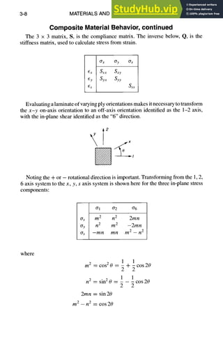
Composite Material Behavior, continued
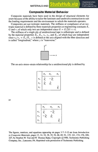
Similarly, for strain transformations,
3-9
61 f2 E6
f x m2 n2 mn
~y n 2 m 2 -mn
Es -2mn 2mn m 2 - n 2
The off-axis in-plane stress-strain relationship is defined by Qij (i, j = 1, 2, 6).
(a) OiJ • (b)
Off-Axis Off-Axis
Strain Strain
El ~2 if6
0"1 Qll Q12 QI6
o2 Q21 Q22 Q26
06 Q61 Q62 Q66
The transformation of on-axis unidirectional properties to off-axis is given by
Qxx Qyy axy Qs,
Q1] m4 n4 2m2n2 4m2n2
Q22 n4 m4 2m2n2 4m2n2
Q12 m2n2 m 2n2 m 4 + n4 -4m2n 2
Q66 m2n2 mZn2 -2m2n2 (m2 - n2)2
Q16 m3n -mn3 mn 3 - m 3n 2(mn3 - m3n)
Q26 mn3 -m3n m 3n - mn 3 2(m3n - mn 3)
m=cos0, n=sin0](https://image.slidesharecdn.com/aiaaaerospacedesignengineersguide-230807164453-d76eba30/85/Aiaa-Aerospace-Design-Engineers-Guide-pdf-65-320.jpg)
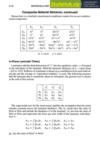
![MATERIALS AND SPECIFICATIONS 3-11
Composite Material Behavior, continued
Flexural Behavior
For flexural behavior, the moment--curvature relationship is the counterpart of
the stress-strain relationship for in-plane behavior. Simplifying for a symmetric
laminate and assuming a linear strain distribution across the thickness of the lam-
inate,
El(z)=zkl
E2(Z)=zk2
66(z)=zk6
where k is curvature with units of in-l or m -1 .
kl k2 k6
M1 DI! D12 DI6
M2 D21 D22 D26
M6 D61 D62 D66
Dll = f QllZ2dz, D22 = f Q22z2dz, D12 = A21
D12 = f Ql2z2dz, D66 = f Q66z2dz, D16 = A61
D16 = f Qi6z2dz, D26 = f Q26z2dz, D26 = A62
General Laminates
For general laminates, coupling exists between flexure and in-plane loading;
this is seen by the addition of Bij terms:
GI
0 G0 G0 kl k2 k6
N1 Al~ Ai2 AI6
N2 A21 A22 A26
N6 A61 A62 A66
M1 Bll B12 B16
M2 B2~ B22 B26
M6 B61 B62 B66
] Bll B12 B16
I Bzl B22 B26
B61 B62 B66
I DIl DI2 D16
I
I D21 D22 D26
[ D6t D62 D66
i
N1 N2 N6 M1 Me M6
GI
0 0/11 0ll2 0/16
G20 0/21 ~22 0/26
G° 0/61 0/62 0/66
kl J~ll ~21 ~61
k2 ~12 ~22 ~62
k6 ~16 J~26 ~66
[ 3. 312 ~16
] ~61 ~62 fl66
t
[ 811 812 816
] 821 822 826
! 861 862 866](https://image.slidesharecdn.com/aiaaaerospacedesignengineersguide-230807164453-d76eba30/85/Aiaa-Aerospace-Design-Engineers-Guide-pdf-67-320.jpg)
![3-12 MATERIALS AND SPECIFICATIONS
Composite Material Behavior, continued
For the symmetric anisotropic laminates, no coupling exists.
~:10 G0 ~) k] k2 k6
NI All AI2 A16 [
N2 A21 A22 A26 [
N 6 A61 At~2 A66 1
I
I
MI [ Dll D12 O16
M2 I D21 D22 D26
M6 [ D61 D62 D66
i
Ni N2 N6 Mt 342 /1//6
¢ 0-,, 0-,2 0-,6 [
I
E2
° O'21 0-22 0-26 1
~:60 0-61 0-62 0-66 I
I
I-
I
kl ~ dll dl2 d16
I
k2 I d21 d22 d26
k6 [ d6t 6/62 d66
For a homogeneous anisotropic laminate, the flexure components are directly
related to the in- plane components.
~10 (20 ~r
0 k 1 k2 k6
Ni All Ai2 AI6 ]
N2 A21 A22 A26 l
N 6 A6t A62 A66 I
i
!
M~ ]
I
M2 [
M6 I
I
h2
Aij
Ni N2 N6 Mt M2 M6
E10 0-11 O"12 (716 [
I
E20 O"21 0"22 0-26 I
~:60 0-61 0"02 0-66 ]
I
kl I
i
k2 I
,,
k6 I
12
~- 0-i
j
Or, in matrix notation,
N = Ae ° + Bk
M = Be ° + Dk](https://image.slidesharecdn.com/aiaaaerospacedesignengineersguide-230807164453-d76eba30/85/Aiaa-Aerospace-Design-Engineers-Guide-pdf-68-320.jpg)


![C
.m
c
o
o
<
c
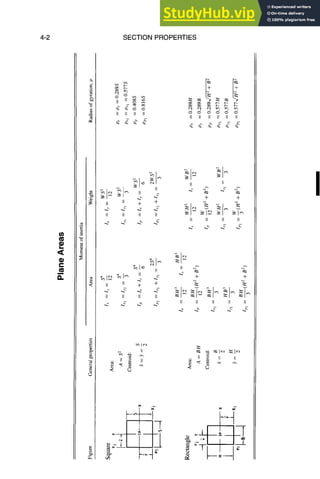
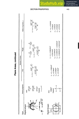
SECTION PROPERTIES
II if II II
II II II
II II II
II II
II [I II II
, , r i
-*
, ~ , , + + +
~l--- ~:1~ ~ ~, ~
II II II If II II
]1 II
L
I
II I1
i ~ I ,,,,~ ,,.,.~
II II II II II II
I
II .~ II
I
II ..~ li II
4-3](https://image.slidesharecdn.com/aiaaaerospacedesignengineersguide-230807164453-d76eba30/85/Aiaa-Aerospace-Design-Engineers-Guide-pdf-72-320.jpg)
![SECTION PROPERTIES 4-17
"0
.m
m
0
t~
.= II c"
II II
II ]1 II
H
H
H
II II II
+ + -t-
II II II
II
II II
Jl ~= , ii ii
x
II
%
II
II
II](https://image.slidesharecdn.com/aiaaaerospacedesignengineersguide-230807164453-d76eba30/85/Aiaa-Aerospace-Design-Engineers-Guide-pdf-86-320.jpg)

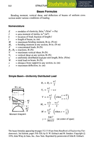
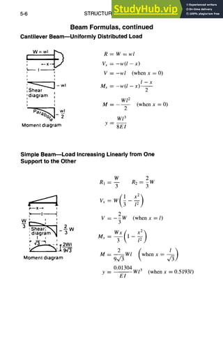
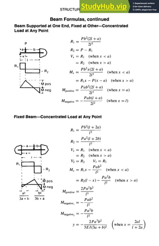
![STRUCTURAL DESIGN
Beam Formulas, continued
Simple BeammConcentrated Load at Any Point
5-3
P
y
IP-X~ I I
L
p--- I ~ ~
I I I
J•x
I ~21 i~o, ,
,diagram '
I !
,' ~'~,~ M ----
Moment diagram y --
y =
RI = P(1 -- k)
R2 = Pk
Vx =R] (whenx <kl)
= -R 2 (when x > kl)
Px(1-k) (whenx <kl)
Pk(1-x) (whenx >kl)
Pkl(1 - k) (at point of load)
3~(1 - k) k -- k2 (when k > 0.5)
3--~k (when k < 0.5)
atx=l(1-/~ -~) (whenk<0.5)
Simple Beam--Concentrated Load at Center
~-- --ll--
I I
p
-- p
2 -~
Shear diagram
I ~,-I---~
,
Moment diagram
P
RI ~ R2 ~ --
2
P
V~= V=+--
2
Mx-- 2
Mx--P(l-x)--2 (whenx>~)
m -- ~ when x =
pl 3
y -- (at center of span)
48EI](https://image.slidesharecdn.com/aiaaaerospacedesignengineersguide-230807164453-d76eba30/85/Aiaa-Aerospace-Design-Engineers-Guide-pdf-103-320.jpg)
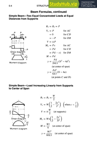
![STRUCTURALDESIGN 5-5
Beam Formulas, continued
Cantilever Beam--Load Concentrated at Free End
, R=P
~ o--X
I
I . V~ =V=-P
I I
- P I i- P Mx = --P(I -- x)
P (
' I M = -PI
Shear diagram
I
I Pl 3
I
I i Y
3El
~ - PI
Moment diagram
(when x = O)
Simple Beam--Load Increasing Linearly from Center to Supports
r-,./1
tx_ : :
wi,,, ,
' ,
- - i
2 Shear~ - W
diagram ' 2
~ T T W I
• ' ~ T'ff
Momen! diagram
W
RI = R2 = --
2
~5 ~) (whenx< ~)
W
V=±--
2
Mx = Wx - 7 + 3-ff,] when x <
Wl
M = -- (at center of span)
12
3W13
y -- (at center of span)
320 E1](https://image.slidesharecdn.com/aiaaaerospacedesignengineersguide-230807164453-d76eba30/85/Aiaa-Aerospace-Design-Engineers-Guide-pdf-105-320.jpg)
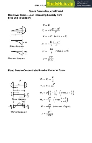
![5-8 STRUCTURALDESIGN
Beam Formulas, continued
Fixed Beam--Uniformly Distributed Load
wl W
RI = R2--
2 2
w1
d W=wl_~ Vx-- 2
x V =±-- (at ends)
,- I ~ 2
'
wJ , wl 2 X X 2
2 [ ' Mx- -
,Shear~l_ wl 2 7 +
idlagram ",, -~-
, w,.__22', M=__lw,2 (whenX=~)
~24 ' 12 x
wl2 ~ ~_' wl2
-q-/g
M -- ~- when x =
W13
y - _ _
384EI
Momentdiagram
Simple BeammUniformly Distributed Load over Part of Beam
wb(2c + b)
R 1 --
2l
wb(2a + b)
R2--
w tb/ft 21
A B.[C" c D wb(2c+b) w(x-a)
~a ]:~- --, V~ -- 21
' ' V=R1 (whena <c)
. 4 I '1
R, [--~i I I = R 2 (when a > c)
i wbx(2c + b)
] - R~ Mx = forAB
IR,~+al i 21
,'w ' "~ - - .Lj M w ( x -- a ) 2
/ ~,_ ~ = RlX 2 forBC
= R2(1 - x) for CD
wb(2c + b)[4al + b(2c + b)]
M=
8/2](https://image.slidesharecdn.com/aiaaaerospacedesignengineersguide-230807164453-d76eba30/85/Aiaa-Aerospace-Design-Engineers-Guide-pdf-108-320.jpg)
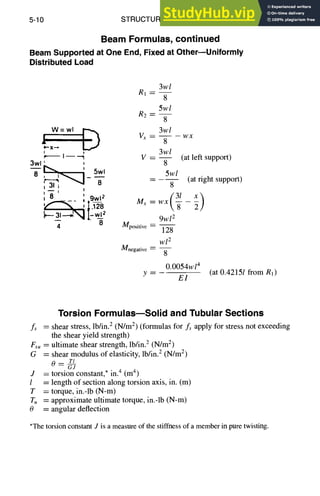
![STRUCTURAL DESIGN 5-13
Torsion Formulas--Thin-Walled Open Sections, continued
i ---~]~"~-- Center
1(2b'~ 4-dt32)
d2Ir
C s --
4
Flange j Y , d
r-q Y,~Ts.ea,
dy], 1 , ~ center
_tECen"o'0
Flange ~ T
no 2 -"~b~ y~"'-t2
tl ~ t2
1
J = 3(bl'~ + b2t3 +dt~)
d21112
Cs--
Iy
Yl Ii -- y212
g--
Iy
Y
Lb I j t,
~rl 'I
~~-r~.ea,
6 T ILK'-' Center
[ t2+ -CentrO'd
~y
!
J = 3(bt3 +dt 3)
C, = 0
Y
T n r I
~ Ce t o d
g2n~lae
r "'~b J ~
Y
CS --
1 3
J = ~(2bt 1 + dt~)
d2ly (1 x(a -
4 r~ x))
xd 2
a--
4~2
Y t~
i f .i
l ~L.,enter
d ~- I T S.ea,
J = ~(2bt 3 + dt32)
d2Ir (l - 3AF~
C~-- 4 -2-A-}](https://image.slidesharecdn.com/aiaaaerospacedesignengineersguide-230807164453-d76eba30/85/Aiaa-Aerospace-Design-Engineers-Guide-pdf-113-320.jpg)
![5-14 STRUCTURAL DESIGN
Position of Flexural (3enter (2 for Different Sections
Form of section Position of Q
Any narrow section symmetri-
cal about the x axis.
Centroid at x = 0, y = 0
' ~
X l ,
~ X
1 + 3v f xt3dx
e-
l + vft3dx
For narrow triangle (with v ----0.25),
e = 0.187a
For any equilateral triangle,
e=0
Sector of thin circular tube
e =
2R
(7r - 0) + sin0 cos0 [(rr - 0)cos 0 + sin0]
For complete tube split along element (0 = 0),
e = 2R
Semicircular area
( 8 3_+4 R
e= 15-7r l+v ] (Q is to right ofcentroid)
For sector of solid or hollow circular area
Angle
Y
1 e @
hi xl Y
e
W
22
h
2
Leg 1 = rectangle wlhl; leg 2 = rectangle w2h2
11 = moment of inertia of leg 1 about Yj (central axis)
12 = moment of inertia of leg 2 about Y2 (central axis)
,
ex = ~h2
(For ex, use xl and x2 central axes.)
1 / 11
eY : 2hl~ l~ )
If wl and w2 are small, ex = ey : 0 (practically) and
Q is at 0.
(continued)
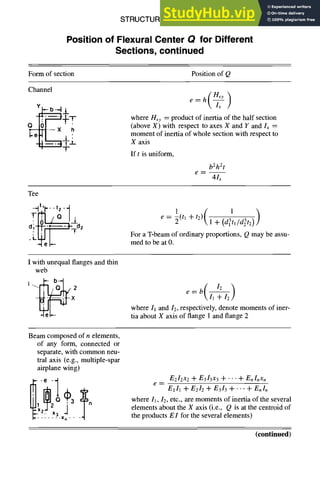
The Position of Flexural Center Q for Different Sections table appearing on pages 5-14-
5-16 is from Formulas for Stress and Strain, 4th Edition, pages 142 and 143, by R. J.
Roark. Copyright @ 1965, McGraw-Hill, New York. Reproduced with permission of The
McGraw-Hill Companies.](https://image.slidesharecdn.com/aiaaaerospacedesignengineersguide-230807164453-d76eba30/85/Aiaa-Aerospace-Design-Engineers-Guide-pdf-114-320.jpg)
![5-16 S
T
R
U
C
T
U
R
A
L
D
E
S
I
G
N
Position of Flexural Center 13 for Different
Sections, continued
Form of section Position of Q
Values of e/h
Lipped channel (t small) ~
~'~c/h~ h 1.0 0.8 0.6 0.4 0.2
Tr~z 0 0.430 0.330 0.236 0.141 0.055
0.1 0.477 0.380 0.280 0.183 0.087
O__.._/ ~ --+-~- -- 0.2 0.530 0.425 0.325 0.222 0.115
04 0 o,6,
/ _LI- q 0.4 0.610 0.503 0.394 0.280 0.155
I.__e__.L_b...] 0.5 0.621 0.517 0.405 0.290 0.161
/ T 1
Hat section (t small)
o z
-LI' ~
Values of e/h
c/h•h 1.0 0.8 0.6 0.4 0.2
0 0.430 0.330 0.236 0.141 0.055
0.1 0.464 0.367 0.270 0.173 0.080
0.2 0.474 0.377 0.280 0.182 0.090
0.3 0.453 0.358 0.265 0.172 0.085
0.4 0.410 0.320 0.235 0.150 0.072
0.5 0.355 0.275 0.196 0.123 0.056
0.6 0.300 0.225 0.155 0.095 0.040
D section (A = enclosed area) ~S/h
t,/ts
-4 0.5
,,"" s " - o 0.6
, , " ~ i th 0.7
- ~ n 0.8
, 0.9
x , 1.0
t 1.2
.o"6
3.0
Values of e(h/A)
1 1.5 2 3 4 5 6 7
1.0 0.800 0.665 0.570 0.500 0.445
0.910 0.712 0.588 0.498 0.434 0.386
-- 0.980 0.831 0.641 0.525 0.443 0.384 0.338
-- 0.910 0.770 0.590 0.475 0.400 0.345 0.305
-- 0.850 0.710 0.540 0.430 0.360 0.310 0.275
1.0 0.800 0.662 0.500 0.400 0.330 0.285 0.250
0.905 0.715 0.525 0.380 0.304 0.285 0.244 0.215
0.765 0.588 0.475 0.345 0.270 0.221 0.190 0.165
0.660 0.497 0.400 0.285 0.220 0.181 0.155 0.135
0.500 0.364 0.285 0.200 0.155 0.125 0.106 0.091](https://image.slidesharecdn.com/aiaaaerospacedesignengineersguide-230807164453-d76eba30/85/Aiaa-Aerospace-Design-Engineers-Guide-pdf-116-320.jpg)

![5-24 STRUCTURAL DESIGN
Columns
Interaction of Column Failure with Local Failure (Crippling)
The method of analysis of columns subject to local failure can be summarized as
follows:
a) Sections having four corners [-]%E
b) Sections having two comers, attached
to sheets along both flanges -l_ E
c) Sections having only two corners but
restrained against column failure about
axis thru comers
% E T_'7_'
(Arrow represents direction of column
failure)
d) Sections having three corners, attached
to a sheet along one unlipped flange -L E
For local failing stress (upper limit of column curve) use crippling stress F,.,. (see note)
e) Sections having only two comers (with "~'*" E-- L--I--
no restraint in any direction)
(Arrow represents direction of column
failure)
f) Sections having only two corners, at-
tached to sheet
-k E
(Arrow represents direction of column
failure)
For local failing stress (upper limit of column curve) use local buckling stress F,~r (see
note)
Column curve For columns that fail by Euler buckling,
select the proper column curve and deter-
mine the allowable ultimate stress Fc.
Note: The calculationsfor F,.,. and F,.r shouldbe madeby referenceto sources not includedin
thishandbook.
Source:Northrop GrummanStructuresManual.Copyright @ Northrop Grumman Corporation,
Los Angeles.Reproducedwithpermissionof NorthropGrumman.](https://image.slidesharecdn.com/aiaaaerospacedesignengineersguide-230807164453-d76eba30/85/Aiaa-Aerospace-Design-Engineers-Guide-pdf-124-320.jpg)
![STRUCTURAL DESIGN 5-25
Columns,continued
Comparison
ofDifferent
Column
Curves
70,000 !
/r Ouc
60,000!/! I
50,000
o~ 40,000
J~
~ 30,000
20,000
10,000
i!/(b) Reduced
--T-~'m°duluscurv'l~,.
] . t l ,
I [
~j (C) Tangen /-()
'O~C,( iq~ i ..~-(e) Straight-
line equation
parabola . ~
Euler columncurve
[ I 1 I
Note: all curves drawn assuming
C=1.0, E=1071b/in. 2 I
0 i [ I i J l
0 20 40 60 80 100 120
L/p
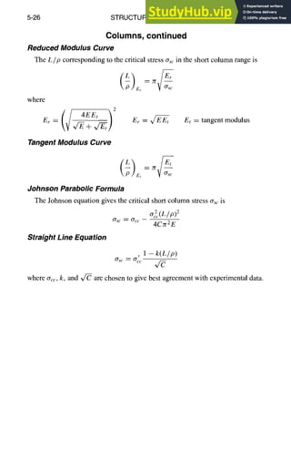
Euler Column Formula
CTr2E I
PE--
L 2
where PE ----critical column load and C = end fixity coefficient (pin end -----1.0,
restrained = 4.0). The critical column stress ~E is
C:rrZE
GE- (L/p)2
where p ----radius of gyration = vf[-/A.
The graph and text appearing on pages 5-25 and 5-26 are from WeightEngineersHandbook,
Revised 1976. Copyright (~ 1976, the Society of Allied Weight Engineers, La Mesa, CA.
Used with permission of the Society of Allied Weight Engineers.](https://image.slidesharecdn.com/aiaaaerospacedesignengineersguide-230807164453-d76eba30/85/Aiaa-Aerospace-Design-Engineers-Guide-pdf-125-320.jpg)
![5-30 STRUCTURAL DESIGN
columns, continued
Column Stress for Aluminum Alloy columns
E
o
50
40
30
20
10
Johnson-Euler formulas
for aluminum columns
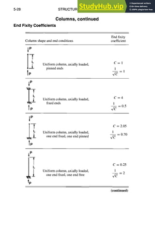
Johnson Formula
Fc = Fcc - Fc%(o~C)2
4r2E
where
C = restraint coefficient
E= 10,300,000 psi
Fc = stress, psi
~ ~ Fcc = crushing stress' psi
Euler Formula
c-~r E~ L ]
O 20 40 60 80 100
L'I~: u(~)
Column Stress for Magnesium Alloy Columns
60~
,,~ 50
9
°
0
0 20
Fc=Fcc- (Fcc)2 L 2
where
Fee = crushing stress, psi
L : column length, in.
p = radius of gyration
C =coefficient of restraint
E = rood. of elas. = 65 x 106 -
40 60 80 100 120
L'lp = L/(p~,/C)](https://image.slidesharecdn.com/aiaaaerospacedesignengineersguide-230807164453-d76eba30/85/Aiaa-Aerospace-Design-Engineers-Guide-pdf-130-320.jpg)

![5-42 STRUCTURAL DESIGN
Forced Vibration, continued
Single Degree of Freedom, continued
The steady-state solution is
x = a sin(wt - 0)
where
as
a =
~/(1--co2/co2)2+[2~(w/mn)] 2
2~(m/mn)
tan 0 --
i - (o~/oJ~)2
a~ : F0/k = maximum static-load displacement
0 = phase angle
= C/Cc = fraction of critical damping
cc = 2x/--m-k = 2row, : critical damping
con = ~,/~/ m, natural frequency, rad/s
'~ 4
" 3
2
j.-[ = 0
I
i___~ = O. I
,11
~.~~~-~0.5
0 0.5 1.0 I.S 2.0 2.5
Frequency ratio, t,o/wn
Forced response of a single-degree-of-freedom system.](https://image.slidesharecdn.com/aiaaaerospacedesignengineersguide-230807164453-d76eba30/85/Aiaa-Aerospace-Design-Engineers-Guide-pdf-142-320.jpg)
![6-2 MECHANICAL DESIGN
Springs
Spring Nomenclature
A = cross-section area of wire, in.2 (m2)
C = spring index = D/d
CL = compressed length, in. (m)
D = mean coil diameter, in. (m)
d = diameter of wire or side of square, in. (m)
E = elastic modulus (Young's modulus), psi (N/m2 = Pa)
FL = free length, unloaded spring, in. (m)
f = stress, tensile or compressive, psi (N/m2 = Pa)
G = shear modulus of elasticity in torsion, E/(2[1 + #]), psi (N/m2 = Pa)
IT = initial tension
in. = inch
J = torsional constant, in.4 (m4)
k = spring rate, P/s, lb/in. (N/m)
L = active length subject to deflection, in. (m)
l = length, in. (m)
lb = pound
N = number of active coils
OD = outside diameter, in. (m)
P = load, lb (N)
P1 = applied load (also P2, etc.), lb (N)
p = pitch, in. (m)
psi = pounds per square inch
r = radius of wire, in. (m)
SH = solid height of compressed spring, in. (m)
s = deflection, in. (m)
T = torque, in.-lb (N-m)
TC = total number of coils
t = leaf spring thickness, in. (m)
U = elastic energy (strain energy), in.-lb (N-m)
w = leaf spring width, in. (m)
/z = Poisson's ratio
zr = pi, 3.1416
r = stress, torsional, psi (N/m 2 = Pa)
Tit = stress, torsional, due to initial tension, psi (N/m 2 = Pa)](https://image.slidesharecdn.com/aiaaaerospacedesignengineersguide-230807164453-d76eba30/85/Aiaa-Aerospace-Design-Engineers-Guide-pdf-148-320.jpg)

![6-18 MECHANICAL DESIGN
Gears, continued
Bevel Gears
a = standard center distance
b
hao
hap =
hfp =
k =
Pe =
z
Znx
(Cperm) , C =
F, =
KI =
K v =
KFa ="
K F/3 =
KFX =
KH~ =
KH~ =
R e =
R m =
T =
YF,(Ys) =
=
E, =
Ztt
Z e
ZR
Zv
Olp
OlW
t~b
p ----
PaO =
O'F lim
O'H lim
tooth width
addendum of cutting tool
addendum of reference profile
dedendum of reference profile
change of addendum factor
normal pitch (Pe = P cos oe,Pet = Pt COSat)
number of teeth
equivalent number of teeth
(permissible) load coefficient
peripheral force on pitch cylinder (plane section)
operating factor (external shock)
dynamic factor (internal shock)
end load distribution factor /
face load distribution factor ] for root stress
size factor
end load distribution factor /
face load distribution / for flank stress
total pitch cone length (bevel gears)
mean pitch cone length (bevel gears)
torque
form factor, (stress concentration factor)
skew factor
load proportion factor
flank form factor
engagement factor
roughness factor
velocity factor
reference profile angle (DIN 867: ceP = 20°)
operating angle
pitch cylinder
skew angle for helical gears base cylinder
sliding friction angle (tan p = #)
tip edge radius of tool
fatigue strength
Hertz pressure (contact pressure)
The gear materialappearing onpages 6-18-6-23 is fromEngineering Formulas, 6thEdition,
McGraw-Hill, New York. Copyright @ 1990, Kurt Gieck, Reiner Gieck, Gieck-Verlag,
Germering, Germany.Reprinted with permission of Gieck-Verlag.](https://image.slidesharecdn.com/aiaaaerospacedesignengineersguide-230807164453-d76eba30/85/Aiaa-Aerospace-Design-Engineers-Guide-pdf-164-320.jpg)
![MECHANICAL DESIGN 6-23
Gears, continued
Calculation of Modulus m
Load capacity of teeth root and flanks and temperature rise are combined in the
approximate formula
Ft2 = C b2 P2 where b2 ~ 0.8 dml and P2 = mzr
0.8T2 Ft2 = 2T2/d2 = 2T2/(m z2)
m ~. q ~ 10fori = 10,20,40
Cpemaqz2 q ~ 17 for i = 80, self-locking
Assumed values for normal, naturally cooled worm gears (worm hardened and
ground steel, worm, wheel of bronze)
Vg ms -1 1 2 5 10 15 20
Cperm Nmm -2 8 8 5 3.5 2.4 2.2
When cooling is adequate this value can be used for all speeds
Cperm > 8Nm m-2
EpicyclicGearing
Presented here is a velocity diagram and angular velocities (referred to fixed
space).
arm fixed wheel
1fixed
1~"~ __ w2=-wl._.....~
~zl °~=°~=(l+r~.....
)
~ ~ ) arm
fixed wheellfixed
s
Wheel
3fixed
°JI= aJs(]-{-r3"~rl
]
_ 2~ arm
fixed wheel
1fixed wheel
4fixed
.
r~ r2r4 rlr3](https://image.slidesharecdn.com/aiaaaerospacedesignengineersguide-230807164453-d76eba30/85/Aiaa-Aerospace-Design-Engineers-Guide-pdf-169-320.jpg)
![6-24 MECHANICAL DESIGN
Formulas for Brakes, Clutches, and Couplings
The kinetic energy E of a rotating body is
E- Igco2 Wk2 N2 Wk2N2
- - - - --x -- ----ftlb
2 g 182.5 5878
where
Ig = mass moment of inertia of the body, lb ft sz
k = radius of gyration of the body, ft 2
W = weight of the body, lb
N = rotational speed, rpm
g = gravitational acceleration, ft/s2
If the angular velocity, co tad/s, of the body changes by AN rpm in t seconds,
the angular acceleration is
2srAN Aco
60t t
The torque T necessary to impart this angular acceleration to the body is
Wk 2 2srAN WkZAN ft
T=Igot= 32.----2x 60t -- 308t
lb
When a torque source drives a load inertia through a gear train, the equivalent
inertia of the load must be used when calculating the torque required to accelerate
the load.
/equivalent Ix~11/ /load
where
]equivalent= equivalent moment of inertia
I2 = moment of inertia of the load
Nl = rotational speed of the torque source
N2 = rotational speed of the load
For example, in the following figure, the equivalent inertia seen by the clutch is
" ( Nz'~2-i-]3(N3~2Nl/
Ul,/
]clutch = It + 12 ~7-~/](https://image.slidesharecdn.com/aiaaaerospacedesignengineersguide-230807164453-d76eba30/85/Aiaa-Aerospace-Design-Engineers-Guide-pdf-170-320.jpg)

![MECHANICALDESIGN
Pumps, continued
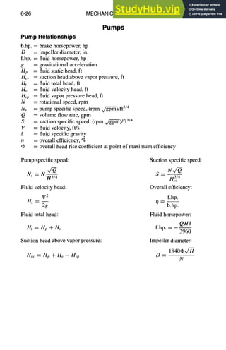
Approximate Relative Impeller Shapes and Efficiencies
as Related to Specific Speed
6-27
100
90
~. 80
0
W
~ 70
L
U.
UI
60
50
40
I i i t I I
I I I I i I t
I b ~ i J i
---,, ~ ,~ -~ ........ ~ ---~---
I i t i l i
, . - - .- . over 10,000 g.p.m.
-I . . . . . ~ - ~ . . . . . r- - - - ~ ~ ~ t- . . . .
i t i ~ t
~ " ', '1 t t
~ ~ 4 ~ t 0 0 to ~ g.p.m. ~ ',
._ ~ ~ o o ~.o~ ..... ~ ..... ~ _ _.
/j,~,~'~" "~; 00 to 2d0 g.p.m.~, ' ~
.~ . _
~ -- ~ _
II l. . . . . . ~L _ L _ _ _ I ]I _ _ ill . . . . . LI --
f ,~T...* t t t i i t
l t t l I
t i I F f
500
RADIAL
1,000 2,000 3,000 4,000 10,000 15,000
SPECIFIC SPEED
FRANCIS MIXED PROPELLER ROTATION
FLOW](https://image.slidesharecdn.com/aiaaaerospacedesignengineersguide-230807164453-d76eba30/85/Aiaa-Aerospace-Design-Engineers-Guide-pdf-173-320.jpg)
![MECHANICAL DESIGN 6-47
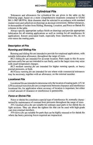
Cylindrical Fits, continued
The following chart provides a graphical representation of the cylindrical fits
provided in the previous table. The scale is thousandths of an inch for a diameter
of one inch.
,- 1
~-2
o
-3
£< m
•
,, m
m RC5 RC8 LT2 LT6 FN2 FN4
m
RC2
m
m
[] HOLES
• SHAFTS](https://image.slidesharecdn.com/aiaaaerospacedesignengineersguide-230807164453-d76eba30/85/Aiaa-Aerospace-Design-Engineers-Guide-pdf-193-320.jpg)
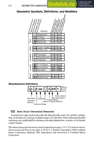
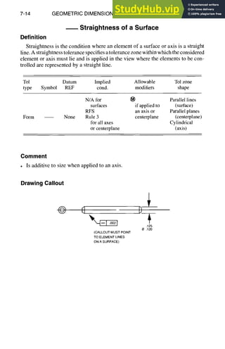
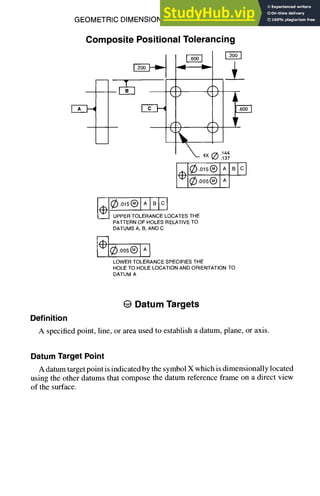
![GEOMETRIC DIMENSIONING AND TOLERANCING 7-5
Geometric Symbols, Definitions, and Modifiers, continued
O Cylindrical Tolerance Zone or Diameter Symbol
Datum Feature Symbol
A datum is the origin from which the location or geometric characteristics of
features of a part are established. Datums are theoretically exact points, axes, or
planes derived from the true geometric counterpart of a specified datum feature.
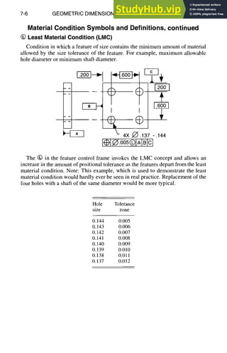
Material Condition Symbols and Definitions
Maximum MaterialCondition(MMC)
Condition in which a feature of size contains the maximum amount of material
allowed by the size tolerance of the feature. For example, minimum hole diameter
or maximum shaft diameter.
~6]-----~
iF-7--O I I +
4X J~ .137-.144
005@IAIBIcI
The ~ in the feature control frame invokes the MMC concept and allows an
increase in the amount of positional tolerance as the features depart from the
maximum material condition.
Hole Tolerance
size zone
0.137 0.005
O.138 0.006
O.139 0.007
0.140 0.008
0.141 0.009
0.142 0.010
0.143 0.011
0.144 0.012](https://image.slidesharecdn.com/aiaaaerospacedesignengineersguide-230807164453-d76eba30/85/Aiaa-Aerospace-Design-Engineers-Guide-pdf-201-320.jpg)
![Additional
GEOMETRIC DIMENSIONING AND TOLERANCING
Standard Rules, continued
Symbols
REFERENCE DIMENSION
PROJECTED TOLERANCEZONE
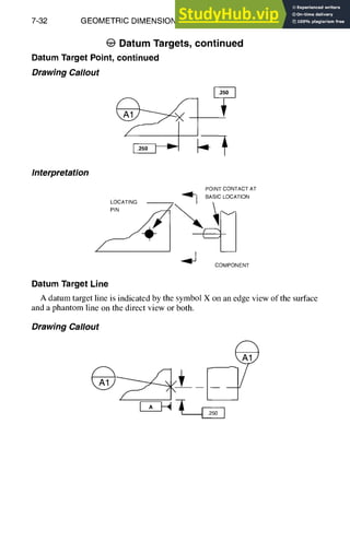
DATUM TARGET
DATUM TARGET POINT
DIMENSION ORIGIN
(5o)
®
®
X
CONICAL TAPER
SLOPE
COUNTERBORE/SPOTFACE I I
COUNTERSINK
DEPTH/DEEP
SQUARE (SHAPE)
DIMENSION NOT TO SCALE
NUMBER OF TIMES OR PLACES
ARC LENGTH
RADIUS
SPHERICALRADIUS
SPHERICAL DIAMETER
ALL AROUND (PROFILE)
BETWEEN SYMBOL
TANGENT PLANE
STATISTICALLY DERIVED VALUE
V
• %-- ,
[]
15
8X
105
SR
s~
.0
@
Q
7-9](https://image.slidesharecdn.com/aiaaaerospacedesignengineersguide-230807164453-d76eba30/85/Aiaa-Aerospace-Design-Engineers-Guide-pdf-205-320.jpg)
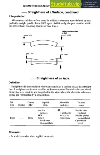
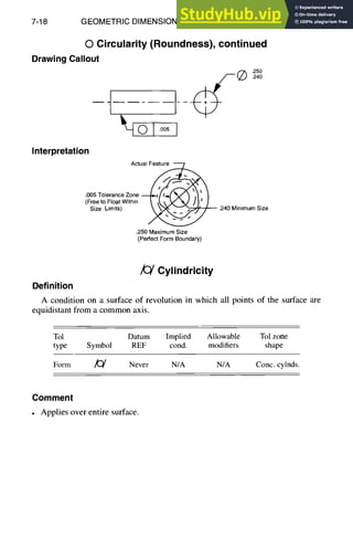
![GEOMETRIC DIMENSIONING AND TOLERANCING 7-19
Drawing Callout
/(~ Cylindricity, continued
. . . . .
Ltc, I .oo I
.250
.240
Interpretation
.250MaxSize
& PerfectFormBoundary
] :::::::::::::::::::::::::::::::::::::
~ T Size
P
nce~ntri!Cy~n;ei ie~ 7a;L; _ _ _ : ............. i
2 Co " " a
.005(Freeto FloatwithinSizeLimits)
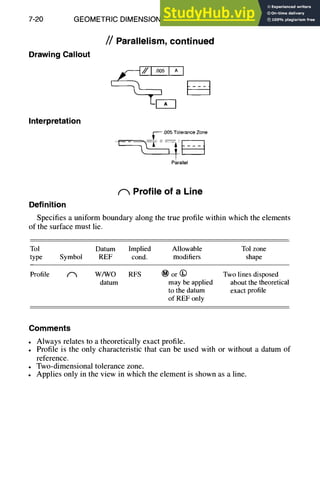
ff Parallelism
Definition
The condition of a surface or axis which is equidistant at all points from a datum
plane or datum axis.
Tol Datum Implied Allowable Tol zone
type Symbol REF cond. modifiers shape
Orientation ff Always RFS @ or (~ Parallel planes
if feature has a (surface)
size consideration Cylindrical
(axis)
Comment
• Parallelism tolerance is not additive to feature size.](https://image.slidesharecdn.com/aiaaaerospacedesignengineersguide-230807164453-d76eba30/85/Aiaa-Aerospace-Design-Engineers-Guide-pdf-215-320.jpg)
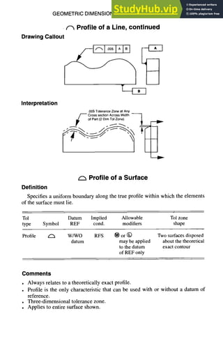
![7-22 GEOMETRIC DIMENSIONING AND TOLERANCING
(~ Profile of a Surface, continued
Drawing Callout
Interpretation
T V-r-1
.005Tolerance Zone
Across Width and ]
Length of Part 1
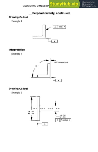
_J_Perpendicularity
Definition
Condition of a surface, axis, median plane, or line which is exactly at 90 deg
with respect to a datum plane or axis.
Tol Datum Implied Allowable Tol zone
type Symbol REF cond. modifiers shape
Orientation _1_ Always RFS ~) or (~) Parallel plane (surface
if feature has a size or centerplane)
consideration Cylindrical (axis)
Comment
• Relation to more than one datum feature should be considered to stabilize the
tolerance zone in more than one direction.](https://image.slidesharecdn.com/aiaaaerospacedesignengineersguide-230807164453-d76eba30/85/Aiaa-Aerospace-Design-Engineers-Guide-pdf-218-320.jpg)
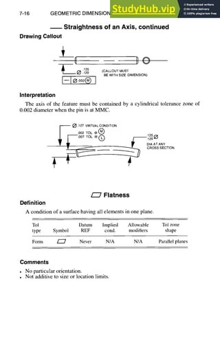
![7-24 GEOMETRIC DIMENSIONING AND TOLERANCING
Interpretation
Example 2
_]_Perpendicularity, continued
.255
(~) Virtual
~ Condition
T Possible
.005 Diametral Axis
Tol at (~ .015 Attitude
Diametral Tol
at©
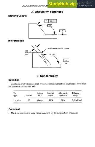
L Angularity
Definition
Condition of a surface, or axis, at a specified angle, other than 90 deg from a
datum plane or axis.
Tol Datum lmplied Allowable Tol zone
type Symbol REF cond. modifiers shape
Orientation L Always RFS ~) or (~) Parallel plane
if feature has a size (surface)
consideration Cylindrical
(axis)
Comments
• Always relates to basic angle.
• Relation to more than one datum feature should be considered to stabilize the
tolerance zone in more than one direction.](https://image.slidesharecdn.com/aiaaaerospacedesignengineersguide-230807164453-d76eba30/85/Aiaa-Aerospace-Design-Engineers-Guide-pdf-220-320.jpg)
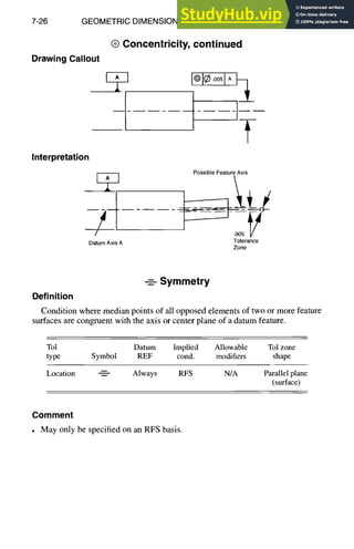
![GEOMETRIC DIMENSIONING AND TOLERANCING 7-27
Drawing Callout
Symmetry, continued
I
Interpretation
1
~ff .Possible
Centerline
I ].O05!ideZone
/ Circular Runout
Definition
A composite tolerance used to control the relationship of one or more features
of a part to a datum axis during a full 360-deg rotation.
Tol Datum Implied Allowable Tol zone
type Symbol REF cond. modifiers shape
Runout / Yes RFS None Individual circular
elements must lie
within the zone
Comments
• Simultaneously detects the combined variations of circularity and coaxial mis-
registration about a datum axis.
• FIM defined as full indicator movement.](https://image.slidesharecdn.com/aiaaaerospacedesignengineersguide-230807164453-d76eba30/85/Aiaa-Aerospace-Design-Engineers-Guide-pdf-223-320.jpg)
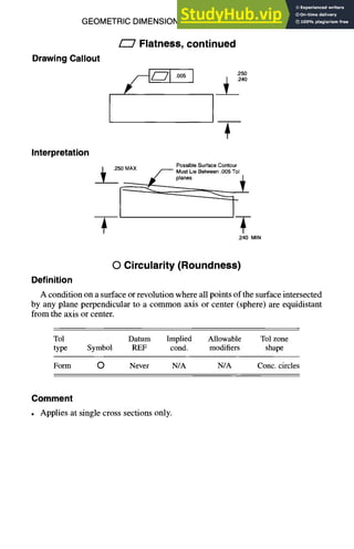
![7-28 GEOMETRIC DIMENSIONING AND TOLERANCING
f Circular Runout, continued
Drawing Callout
I"10051~~
I"l°°51A~" ~-.1 I ,
Interpretation
.005FIMAtlowe~
ateachCircular
ElementWith/ndicator
Held
i InaFixedPosition
.~ = PartRotated360deg
onDatumAxisA
~ Single
Circular
Elements
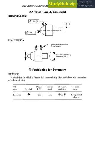
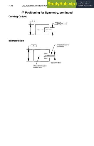
Total Runout
Definition
A composite tolerance used to control the relationship of several features at
once, relative to a datum axis.
Tol Datum Implied Allowable Tol zone
type Symbol REF cond. modifiers shape
Runout ~ Always RFS N/A L'r ] "005 I A I
FIM
Comments
• Can be defined as the relationship between two features.
• May only be specified on an RFS basis.
Simultaneously detects combined errors of circularity, cylindricity, straightness,
taper, and position.](https://image.slidesharecdn.com/aiaaaerospacedesignengineersguide-230807164453-d76eba30/85/Aiaa-Aerospace-Design-Engineers-Guide-pdf-224-320.jpg)


![8-8 ELECTRICAL/ELECTRONIC/ELECTROMAGNETIC DESIGN
Resistor, Capacitor, Inductance Combinations
Parallel Combinations of Resistors, Capacitors, and Inductors
Magnitude of
Parallel Impedance, ohms impedance, ohms
combination (Z = R + jX) (IZI = ~ X 2)
R1R2 R1R2
R1, R2
R1 + R2 R1 + R2
1 1
C1, C2 j co(CI ~- C2) co(C1 ~- C2)
coZLZR + jcoLR 2 mLR
L,R
CO2L2+ R2 ~/CO2L2+ R2
R - jcoRzC R
R,C
1 ~t_co2R2C2 ~/l + CO2R2C2
wL coL
L, C +J 1 - m2LC 1 - co2LC
L1L2 - M 2 L]L2 - M2
LI(M)L2 +jw co
La + L2 qz 2M L1 + L2 q: 2M
( ,) /j ( l;
L, C, R T - i coC R I+R 2 COC
coL coL
Parallel Phase angle, rad Admittance, siemens
combination [4) = tan I(X/R)] (Y = 1/Z)
R1 +R2
R1, R2 0
R1R2
7/
C1, C2 +jco(C1 + C2)
2
R l j
L, R tan-~ --
coL R coL
1
R,C tan-l(-coRC) ~ + jcoC
L,C -~ j wC
75.,1
(LI_+ LzTZM~
7g
-J~u L1L2 - m 2 ]
LI(M)L2 ±2
L,C,R tan 1-R(wC ~)](https://image.slidesharecdn.com/aiaaaerospacedesignengineersguide-230807164453-d76eba30/85/Aiaa-Aerospace-Design-Engineers-Guide-pdf-241-320.jpg)
![ELECTRICAL/ELECTRONIC/ELECTROMAGNETIC DESIGN 8-9
Resistor, Capacitor, Inductance Combinations, continued
Series Combinationsof Resistors,Capacitors,and Inductors
Magnitude of
Series Impedance, ohms impedance, ohms
combination (Z = R + jX) (IZ[ = ~ + X 2)
R R R
L +jcoL coL
C -j(1/wC) 1/wC
R1 + R2 Rj q- R 2 R1 q- R2
Lj(M)L~ +jw(L1 + Le 4- 2M) co(L1 + L2 + 2M)
11c,+c2"~ 1(c,+c2)
c, +c2 ~ c-GG- ) ~ c--EG-)
R + L R + jcoL ~/R2 + c02L2
1 /w2C2R 2 + 1
R q-C R- j w~ */v ~2
(1) ((l)
R + L + C R + j coL o~C R2+ WL - o~C
Series Phase angle, rad Admittance, siemens
combination [q5 = tan-1 (X/R)] (Y = 1/Z)
R 0 1/R
L +re/2 -j(l#oL)
C -re~2 jogC
R 1 q- R 2 0 1/(Rj + R2)
LI(M)L 2 +rr/2 -j/og(L1 + L2 -4-2M)
Y'( . [" GIG 2 "~
c,+c2 2 J'°~,c--,~)
ogL R - jwL
R + L tan-1 __
R R 2 q- 092L2
l wzCZR+ jcoC
R + C -tan -l - -
coRC w2C2R2 + 1
zr j coC
L+C 4---
2 w2LC - 1
(09L -_ l/coC ) R - j(09L -1/o>C)
R + L + C tan-1 R2 + (wL - l/~oC)2](https://image.slidesharecdn.com/aiaaaerospacedesignengineersguide-230807164453-d76eba30/85/Aiaa-Aerospace-Design-Engineers-Guide-pdf-242-320.jpg)
![ELECTRICAL/ELECTRONIC/ELECTROMAGNETIC DESIGN 8-11
Dynamic Elements and Networks, continued
DC-Motor, Field Controlled
O(s) Km
Vf(s) s(Js + f)(Lfs + R f)
DC-Motor, Armature Controlled
R a La
Va(S)~wl
Vbl
C
O(s) gm
Va(s) s[(Ra -t- Las)(Js q- f) -t- KbKm]
Laplace Transforms
The Laplace transform of a function f(t) is defined by the expression
F(p) = f(t)e -p' dt
If this integral converges for some p = Po, real or complex, then it will converge
for all p such that Re(p) > Re(p0).
The inverse transform may be found by
f
c+joo
f(t) = (j27r) -1 F(z)e tz dz t > 0
v c--joo
where there are no singularities to the fight of the path of integration.
Re (p) denotes real part of p
lm (p) denotes imaginary part of p
The Laplace transform material appearing on pages 8-11-8-13 is from Reference Datafor
Engineers: Radio, Electronics, Computer,and Communications, 8th Edition, page 11-36.
Copyright (~) 1993, Butterworth-Heinemann, Newton, MA. Reproduced with permission
of Elsevier.](https://image.slidesharecdn.com/aiaaaerospacedesignengineersguide-230807164453-d76eba30/85/Aiaa-Aerospace-Design-Engineers-Guide-pdf-244-320.jpg)
 + azFz(p)
-f(O) + pF(p)
P-ll f f(t)dt]t=o+[f(P)/P],
Rep > 0
~r f('~)e-px __ e-Pr), 0
d)~/(l r >
fo r f()~)e-~ + e-Pr), 0
d,k/(1 F >
F(p/a)/a
F(p -a), Re(p) > Re(a)
(- 1)"[dnF(p)/dp"]
lim pF(p)
p--~0
lim pF(p)
aF(p) denotes the Laplace transform of f(t).
Miscellaneous Functions
Function Transform
Step
Impulse
u(t - a) = O, 0 < t < a e ap/p
= 1, t>a
8(0 l
t~, Re(a) > -1 F(a + 1)/p a+a
e"t 1/(p - a), Re(p) > Re(a)
t"ebt, Re(a) > -1 F(a + 1)/(p - b)a+l, Re(p) > Re(b)
cos at p/(p2 + a2)|
sinat a/(p 2 q- a2) "
~Re(p) IIm(a)l
>
(continued)](https://image.slidesharecdn.com/aiaaaerospacedesignengineersguide-230807164453-d76eba30/85/Aiaa-Aerospace-Design-Engineers-Guide-pdf-245-320.jpg)
![ELECTRICAL/ELECTRONIC/ELECTROMAGNETIC DESIGN
Laplace Transforms, continued
Miscellaneous Functions, continued
8-13
Function Transform
cosh a t
sinhat
~t
1/(t+a), a >0
e at2
Bessel function Jv (a t),
Re(v) > - 1
Bessel function Iv(at),
Re(v) > - 1
p/(p2 _ a 2) i
l/(p 2 -- a 2) "IRe(p) IRe(a)l
-(y + f~p)/p, y is Euler's constant = 0.57722
eapEl (ap)
½(rc/a)l/2epZ/n%rfc[p/2(a) 1/2]
r-l[(r - p)/a] v, r =(p2 + a2)1/2, Re(p) > IRe(a)l
R-I[(R - p)/aff, R =(p2 _ a2)1/2, Re(p) > IRe(a)]
InverseTransforms
Transform Function
1 3(t)
1/(p + a) e-at
1/(p + a)v, Re(v) > 0 t v le-at/I'(v)
1/[(p + a)(p + b)] (e.... e b')/(b -- a)
p /[(p + a)(p + b)] (ae .... be-bt)/(a -- b)
1/(p 2 + a 2) a -l sinat
1/(p 2 - a 2) a -1 sinh at
p/(p2 + az) cosat
p/(p2 _ a 2) coshat
1/(p 2 + a2) 1/2 Jo(at)
e-aP/p u(t - a)
e-aP/p v, Re(v) > 0 (t - a)V-lu(t - a)/F(v)
(1/ p)e -alp Jo[2(at)1/2]
(1/ pV)e a/p ]~ , , (t/a)(v-l)/2 jv_l [2(at)l/2]
(1/pv)ea/p IKew) > 0 (t/a)~V_W2lv_l[2(at)i/2]
(l/p) Gp --y -- Gt, 2/ = 0.57722](https://image.slidesharecdn.com/aiaaaerospacedesignengineersguide-230807164453-d76eba30/85/Aiaa-Aerospace-Design-Engineers-Guide-pdf-246-320.jpg)
![8-14 ELECTRICAL~ELECTRONIC~ELECTROMAGNETIC
DESIGN
T
F
H
~k
Electromagnetic Symbol Definition
il
f')~=c
k
Ikl = k 9.r
E 377 ohms
Z:T]°-- n --
~= ~: × ~I
1 H 2 1 E 2
W = ~#. + ~e.
#
S
Electric field (volts/meter)
Magnetic field (amps/meter)
Frequency (f) and wavelength (~.)
related by velocity of propagation (c)
Direction of propagation
Propagation constant (1/meter)
Impedance of free space
Energy flow (watts/meter2)
Energy density
Complex permeability
Complex permittivity
Electromagnetic Spectrum (Wave Length vs Frequency)
Frequency (MHz)
o o z o o o o o o o o . . . . . . .
x ~ x x x x . K ~ × x x ~ × x x
03 eo o3 ¢0 03 03 ¢0 co co eo 03 co ¢q 03 03 03 o~ o~ 03
Hertzian waves ,
.c,o I
waves ~ e
~ " ~ --Cosmic rays--~
Wavelength (A) . . . . : | L ~ '~, ~
~x~O~A ~xi°~Ai ~x,O~Ai 4,,0~A
Orange Yellow ] Viole
.ed I IOr;on
Infrared ~ ~ Ultraviolet
Speed of light = 3 x 101°cm/sec White Light ;~ =5500 A
1 micron = 10 "4 cm White Light ~, =0 00022 inches
1 Angstrom unit (A) = 10 "8 cm White Light ~, =0.00055 mm
P1 Vl 11
- - - - = 20 log1
db=10 log10 P2 db=20 Ioglo V2 0"~-
2
Source: WeightEngineers Handbook, Revised 1976. Copyright (~ 1976, the Society of
Allied Weight Engineers, La Mesa, CA. Reproduced with permission of the Society of
Allied WeightEngineers.](https://image.slidesharecdn.com/aiaaaerospacedesignengineersguide-230807164453-d76eba30/85/Aiaa-Aerospace-Design-Engineers-Guide-pdf-247-320.jpg)
![ELECTRICAL/ELECTRONIC/ELECTROMAGNETIC DESIGN 8-21
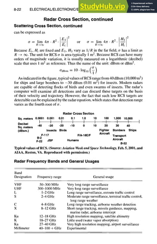
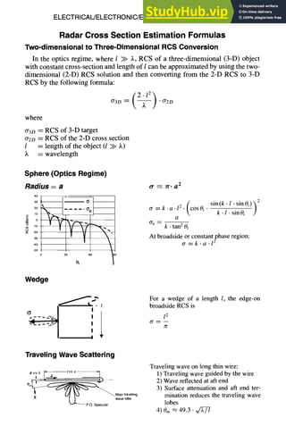
Radar Cross Section, continued
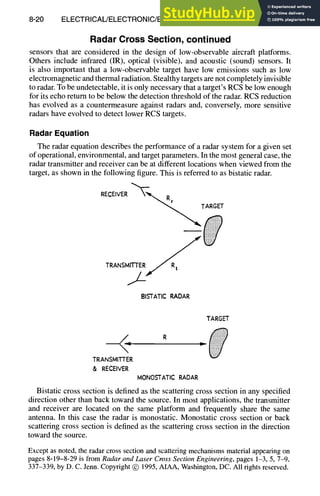
The radar equation is usually written as
PT " DT " DR • cr • 3.2
PR ~- (47r)3 . R4
or
Rmax = I PT " DT " DR ")~2"a ]
where
R = distance between monostatic radar and target
Pv = radar transmitting power
PR = radar receive power
DR = transmitting antenna directivity
Dr = receiving antenna directivity
¢r = target "cross section" or radar cross section
~. = wavelength
For a given scattering object, upon which a plane wave is incident, that portion
of the scattering cross section corresponding to a specified polarization component
of the scattered wave is considered the RCS.
Scattering Cross Section
The RCS for a scattering object, upon which a plane wave is incident, is consid-
ered to be that portion of the scattering cross section corresponding to a specified
polarization component of the scattering wave.
The RCS of a target can be simply stated as the projected area of an equivalent
isotropic reflector that returns the same power per unit solid angle as the target
returns; it is expressed by
where
P/
Ps
or-P/
o-.P/
-- Ps • R2
4Jr
= power density incident on target
= power density scattered by target
4zr = power scattered in 4zr steradians solid angle
Ps • R2 = power per unit solid angle reflected to the receiver
Because RCS is a far-field quantity, RCS can then be expressed as
cr= lim (47rR2"~
- ) R - - , ~
Power density can be expressed in terms of electric or magnetic fields, and RCS](https://image.slidesharecdn.com/aiaaaerospacedesignengineersguide-230807164453-d76eba30/85/Aiaa-Aerospace-Design-Engineers-Guide-pdf-254-320.jpg)
![ELECTRICAL/ELECTRONIC/ELECTROMAGNETIC DESIGN 8-25
Scattering Mechanisms, continued
will be reflected back toward its origin. Traveling wave RCS lobes can achieve
surprisingly large levels.
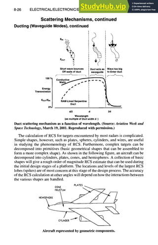
A metallic sphere of radius a is commonly used as a calibration target for RCS
measurement; its RCS vs circumference in wavelengths ka is illustrated below.
This figure also illustrates three frequency regimes that are applicable to general
targets. For small ka (k >> a) the RCS of the sphere is cr/zra 2 = 9 • (ka) 4. This
is also known as the Rayleigh scattering law, which is applicable when k is large
in comparison with the target characteristic dimension. The oscillatory nature of
the resonance (Mie) region results from the interference between creeping waves
and specular reflected waves. At very large ka (k << a), the scattering behavior is
similar to optical scattering; i.e., cr/~a 2 = 1. In this regime, simple formulas can
be derived for several canonical shapes assuming that the phase of the wavefront is
constant across the impinged target area. The term "constant phase region" refers
to this approximation for RCS at very high frequency.
°l :
1 A4^, .....
]~2 .1
"01L~RAYLEIG H~RESONANCE~L OPTICs
..,V.-,O.T ..o,o. T.-,o.
.1 1 10 100
Im
RCS of a metallic sphere with radius of a. (Source: Radar Cross Section, page 53,
figure 3-5, by Knott, Schaeffer, and Tuley. Copyright (~)1985, Artech House Publishers,
Norwood, MA. Reproduced with permission of Artech House, www.artechhouse.com.)
Ducting(WaveguideModes)
Ducting occurs when a wave is trapped in a partially closed structure. An exam-
ple is an air inlet cavity on a jet propelled vehicle. At high frequencies, where the
wavelengths are small relative to the duct dimensions, the wave enters the cavity
and many bounces can occur before a ray hits the engine face and bounces back
toward the radar, as illustrated in the following figure. The ray can take many paths,
and therefore, rays will emerge at most all angles. The result is a large, broad RCS
lobe. In this situation, radar absorbing material (RAM) is effective in reducing the
backscatter. At the resonant frequencies of the duct, waveguide modes can be ex-
cited by the incoming wave. In this case the use of RAM is less effective. At lower
frequencies, where the wavelength is relatively larger than the duct dimensions, no
energy can couple into the duct and most of the scattering occurs in the lip region
of the duct.](https://image.slidesharecdn.com/aiaaaerospacedesignengineersguide-230807164453-d76eba30/85/Aiaa-Aerospace-Design-Engineers-Guide-pdf-258-320.jpg)

![9-2 AIRCRAFT AND HELICOPTER DESIGN
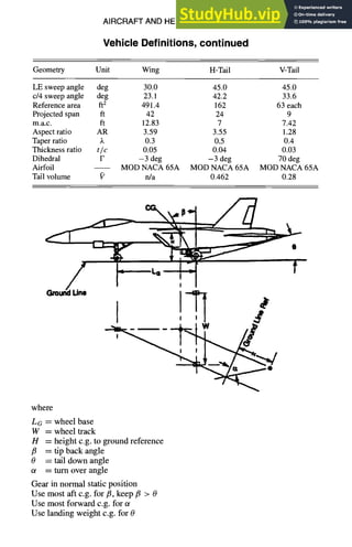
Vehicle Definitions
Geometry
The following figures and formulas provide an introduction on geometric re-
lationships concerning vehicle physical dimensions. These dimensions are used
throughout this section.
WING
45DEG
HORIZONTAL
TAIL
(~ / ~)~ .I
~ . .... 18FT.... ~'11 C
H
o
R
D
R
O
O
T. TAIL
SPAN24
FT
~ ~ _ _ ~ ] ~ ~ T?MAFCT
~ I
I~" 9FT
C/4SWEEP/ M A ~ F ~ L ~ b ...1
=~--, ,, 'T~iL;~ffM'- -'-I-,'I4.SFTI"-
/ ~" 18FT TIPCHORD
LEoS~EEEP " ~ /
--=~ 5.4FT ~-
TIPCHORD
TIPCHORD
.=~i 4
~=_~.~/S VERTICAL
TAIL
I VERTICAL/ // F" f f
COCKPIT ~ TAILARM~ MAC / TAILSPAN /
PILOTVISION ~ 14F A • ,-
T 9 FT HEfGHT
13D E G - ' ~ 1 ~ 9 ; T 18FT
, '
I'u OVERALLLENGTH60FT m
I WINGSPAN4.2FT
II FOLDEDSPAN33FT ---'
I
/ VERTICAL k i I
ITAILDIHEDRAL~ ,I
.?, ,ODEG~ ,~ /
iI -- i1,
/ , ~ ~ ~ h" 4 ., WINGDIHEDRAL
J ~ ~ -3DEG
HORIZONTAL ~ ~'% ~ 40- 45DEG
TAILDIHEDRAL
L " " OVERSIDEVISIONANGLE
-3DEG ~DI WHEELTRACKll~
/ 11FT /](https://image.slidesharecdn.com/aiaaaerospacedesignengineersguide-230807164453-d76eba30/85/Aiaa-Aerospace-Design-Engineers-Guide-pdf-264-320.jpg)
![9-4 AIRCRAFT AND HELICOPTER DESIGN
Vehicle Definitions, continued
Geometry, continued
The following definitions and equations apply to trapezoidal planforms, as
illustrated here.
r S~/m(~ r
''I"1
_I.
0,4
~= b/2 =
"~ b
~Y
,p,,
{:
LE /
r AXE ~ r _ S f C°
. r ~,
-I
x
Co = overall length of zero-taper-ratio planform having same leading- and
trailing-edge sweep as subject planform
(~ = ratio of chordwise position of leading edge at tip to the root chord length
= (b/2) tan ALE(1/Cr)
7,. 72 = span stations of boundary of arbitrary increment of wing area
Am, A. = sweep angles of arbitrary chordwise locations
rn, n = nondimensionalchordwise stations in terms of C
General
y
7=
b/2
~. = C,/Cr
C = Cr[1 - 7(1 - X)]
tan A = 1/ tan E
XLE = (b/2)7 tan ALE
b 1 - aZ
= - tan ALE + Ct = Cr - -
2 1-a
Area
b 2 b b
S -- AR -- 2 Cr(1 +X) -----~Co(1 -a)(1 -X)
CoZ(1 - a)(1 - Z2)
tan ALE
b -ql
AS = ECr[2 - (1 - )v)(71 - 02)] 72](https://image.slidesharecdn.com/aiaaaerospacedesignengineersguide-230807164453-d76eba30/85/Aiaa-Aerospace-Design-Engineers-Guide-pdf-266-320.jpg)
![AIRCRAFT AND HELICOPTER DESIGN 9-5
Vehicle Definitions, continued
Aspect Ratio
AR--
b 2
S
2b 4(1 - X)
Cr(l q- )~) (1 -- a)(1 + X)tan ALE
Cutout Factor
a D
tan ATE Cr(1 - ~) 4(1 - )~)
- - -1 -1-
tan ALE (b/2)tan ALE AR(1 + X)tan ALE
Sweep Angles
1 Cr(1 - X) 4(1 - X)
tan ALE : -- tan ATE --
a (b/2)(1 - a) AR(1 + X)(1 - a)
Co(1 - X) AR(1 q- )~)tan Ac/4 -1-(1 - ~,) 4 tan Ac/4
b/2 AR(1 + X) 3 + a
tan A m = tan ALE[1 -- (1 - a)m]
tan Am = tan ALE -- ~--~ ]-~
1
cosAm=tanALE,-,{1 )2
G~LE "[-[1 -- (1 -- a)m] 2
Mean Aerodynamic Chord (m.a.c.)
2f b/2 2 ( )v2 )
e=~,o C2dy=~Cr 1+ 1~- ~
= 5Co(1 - a) +
1
4 S ~ X
2( CrxC~t
)
= -~ Cr + G Cr-7-
2 fb/2 1 -- ((J/Cr)
rl = S., o Cy dy -- 1 - )v --
1
3l+X/
XLE = y tan ALE](https://image.slidesharecdn.com/aiaaaerospacedesignengineersguide-230807164453-d76eba30/85/Aiaa-Aerospace-Design-Engineers-Guide-pdf-267-320.jpg)
![AIRCRAFT AND HELICOPTER DESIGN 9-7
Aerodynamics
BasicAerodynamicRelationships
AR = aspect ratio = b2/S
Co = drag coefficient = D/qS = Coo + Col
CDi = induced drag coefficient = CeL/(rcARe)
CL = lift coefficient = L/qS
Ct = rolling-moment coefficient = rolling moment/qbS
Cm = pitching-moment coefficient = pitching moment/qcS
Cn = yawing-moment coefficient = yawing moment/qbS
Cy = side-force coefficient = side force/qS
D = drag = CDqS
d = equivalent body diameter = ~/4AMAx/Yr
FR = fineness ratio = £/d
L = lift = CLqS
M = Mach number = V/a
P = planform shape parameter = S/be
q = dynamic pressure = ½(PV 2) = ½(pa2M2)
Rn = Reynolds number = Vgp/tz
Ro = d/2 = equivalent body radius
(t/C)RMS= root-mean-square thickness ratio
1
i1 [b/2 2dy]~
(t/C)RMS ~- b/2- r~r (t/c)
V = true airspeed = Ve/ff1/2
= chordwise location from apex to C/Z (equivalent to chordwise loca-
tion of centroid of area)
=- cx+ y
Sjo
)¢LE = chordwise location of leading edge of m.a.c.
XLE ~ X -- --
2
I? = spanwise location of C (equivalent to spanwise location of centroid of
area)
2 fb/2
= -- cy dy
Suo
/~ = ~ - 1 (supersonic), ~/1 -- M 2 (subsonic)
= complement to wing sweep angle = 90 deg--ALE
O = nondimensional span station = y/(b/2)
)~ = taper ratio, tip-to-root chord = Ct/Cr
a = air density ratio = P/Po
v = kinematic viscosity = #/p](https://image.slidesharecdn.com/aiaaaerospacedesignengineersguide-230807164453-d76eba30/85/Aiaa-Aerospace-Design-Engineers-Guide-pdf-269-320.jpg)
![9-12 AIRCRAFT AND HELICOPTER DESIGN
Aerodynamics, continued
AirspeedRelationships
IAS --indicated airspeed (read from cockpit instrumentation, includes cockpit-
instrument error correction)
CAS--calibrated airspeed (indicated airspeed corrected for airspeed-instru-
mentation position error)
EAS--equivalent airspeed (calibrated airspeed corrected for compressibility
effects)
TAS--true airspeed (equivalent airspeed corrected for change in atmospheric
density)
EAS
TAS --
Mach number:
where
Va = true airspeed
a = sonic velocity
y = specific heat ratio
g = gravitational constant
R = gas constant
T = ambient temperature
M -- vo - vo/,/7 Rr
a
Change in velocity with change in air density, p, at constant horsepower, hp:
V2 = Vl ,3//~]S (approximate)
V /92
Change in velocity with change in horsepower at constant air density:
3/hp2 (approximate)
V2= V1V hpl
The following are equivalent at 15,000 ft, 30°C day:
M = 0.428
TAS = 290 kn
CAS = 215 kn
EAS = 213 kn](https://image.slidesharecdn.com/aiaaaerospacedesignengineersguide-230807164453-d76eba30/85/Aiaa-Aerospace-Design-Engineers-Guide-pdf-274-320.jpg)
![9-14 AIRCRAFT AND HELICOPTER DESIGN
Aerodynamics, continued
Airspeed Conversion Charts, continued
n"
LU
t,n
Z
~ .40
0
PRESSUREALTITUDE,103FT
50 40 30 20 10
.50 500
~,..] B Soo
/, / I'~.~ / oO/ 400
~20 200
','o ,,.:~ A CAS=215kt
~ ~i B Altitude=15,000ft
C M =.428
D TAS (ICAOstd. day)=268 kt
| E Tam=30°C I
I F TAS=290kt
l
.10 !A| j 100
100 200 300 400
CALIBRATEDAIRSPEED,KNOTS
CB
I--
O
Z
v
d
W
ILl
O.
C
S
~
rr
W
rr](https://image.slidesharecdn.com/aiaaaerospacedesignengineersguide-230807164453-d76eba30/85/Aiaa-Aerospace-Design-Engineers-Guide-pdf-276-320.jpg)
![9-16 AIRCRAFT AND HELICOPTER DESIGN
Aerodynamics, continued
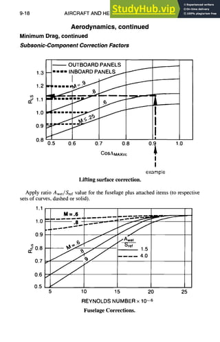
MinimumDrag
Subsonic
The basic minimum drag of an aerodynamic vehicle consists of not only friction
drag but also drag due to the pressure forces acting on the vehicle.
The following equations present a method of predicting minimum drag:
Minimum drag = Comi.qS
~_,(Cfoomp )< z .... p)
C Omin = S -~- COcamber -~- CDbase -~- C Omisc
where the component skin-friction coefficients are evaluated according to the fol-
lowing equations.
Awcomp
C
Cfcom p =
C fwing =
Cffuselage =
Cfnacelle =
C fcanopy =
C fhoriz&verttails(onepiece)
C fhoriz&verttails(hinged)
CL........ =
CD~.mbe~
C Dbase
CDmin
CDmi~c
CfFP =
FR =
component wetted area
lifting surface exposed streamwise m.a.c.
component drag coefficient
CfFp[1 + L(t/c) + lO0(t/c)4]Res
Cf~[1 + 1.3/P--Ii,15 + 44/F-t~3]Rfus
CSF
P × Q[1 + 0.35/(F--1~)1
CfFp[1 + 1.3/Fl~15 -Jr44/F--I~3]
Cf~[1 + L(t/c) + lO0(t/c)4]Rts
(1.1)CfFp[l + L(t/c) -I- lO0(t/c)a]Rts
CfFo X Q[1 + 1.3/F-R1'5 + 44/~ 3]
0.7(AC2)(SExp/S) (do not use for conical camber)
base drag: a good estimate can be obtained by using a base
pressure coefficientof Cp = -0.1. (More detailed discussion
of base drag may be found in Hoerner's Fluid Dynamic Drag.)
minimum drag coefficient
miscellaneous drag coefficient
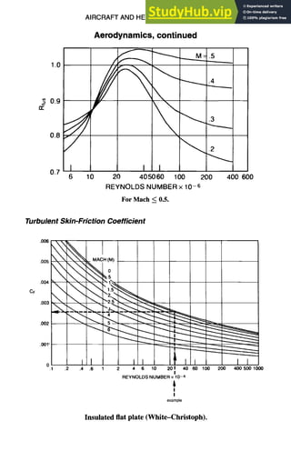
White-Christoph's flat-plate turbulent-skin-friction coeffi-
cient based on Mach number and Reynolds number (in which
characteristic length of lifting surface equals exposed m.a.c.)
fineness ratio
length/diameter (for closed bodies of circular cross section)
length/~/(width)(height) (for closed bodies of irregular cross
section and for nacelles)
/ V/ 1 (1 ~) (~)2 (for closed bodies of elliptic
length a 1-4-g -
cross section, where a = minor axis and b = major axis)](https://image.slidesharecdn.com/aiaaaerospacedesignengineersguide-230807164453-d76eba30/85/Aiaa-Aerospace-Design-Engineers-Guide-pdf-278-320.jpg)
![AIRCRAFTAND HELICOPTERDESIGN
Aerodynamics, continued
Lift Effect on Critical Mach Number (For Conventional Airfoils)
1.0
o
t4
i
.9
~
.8
9-25
.o2 //o
.06 .1--
.08
'16 18
2 g ~
.4
.18
.5
Drag Rise
Following the critical Mach number, the drag level increases abruptly. This
phenomenon is associated with strong shocks occurring on the wing or body,
causing flow separation. To estimate the drag rise increment at these conditions,
Hoerner, in Fluid Dynamic Drag, gives the following empirical relation.
ACDR,se=(K/IO3)[IOAM/(cos1-ALE
MCR)]n
where
K = 0.35 for 6-series airfoils in open tunnels
= 0.40 for airfoil sections with tic ~ 6%
= 0.50 for thicker airfoils and for 6-series airfoils
AM = M - MCR
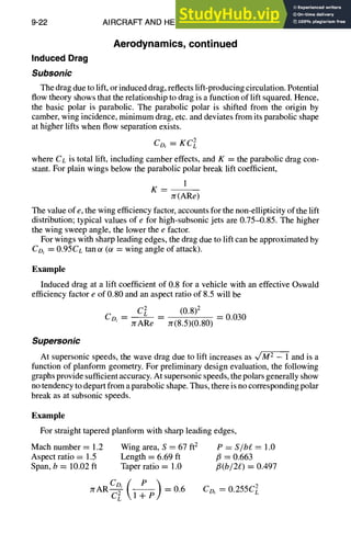
n = 3/(1 + ~-~R)](https://image.slidesharecdn.com/aiaaaerospacedesignengineersguide-230807164453-d76eba30/85/Aiaa-Aerospace-Design-Engineers-Guide-pdf-287-320.jpg)
![9-26 AIRCRAFT AND HELICOPTER DESIGN
Aerodynamics,continued
Drag Rise, continued
Example
Determine the drag rise increment for the following.
AM ----0.05
Aspect ratio = 3.0
t/c = 0.068 (K = 0.40)
ALE = 50 °
McR = 0.895
0.4 F 10(0.05) ] ,+-]/3
mfoRise -- 1000 kcos(5~ i ~-0.895
= 0.0002136
Aerodynamic Center
The prediction of wing-alone aerodynamic center (a.c.) may be made from
curves presented in the following graphs which show a.c. location as a fraction of
the wing root chord. These curves are based on planform characteristics only and
are most applicable to low-aspect-ratio wings. The characteristics of high-aspect-
ratio wings are primarily determined by two-dimensional section characteristics
of the wing.
The wing is the primary component determining the location of the airplane a.c.,
but aerodynamic effects of body, nacelles, and tail must also be considered. These
effects can be taken into account by considering each component's incremental
lift with its associated center of pressure and utilizing the expression,
CM~
a.c.--
CL~
Example
Determine the location of the aerodynamic center of a wing under the following
conditions.
Machnumber = 1.2 (fl = 0.663)
ALE = 45 deg
Aspect ratio = 2.0
Taper ratio (~.) = 0.2
Xac
-- 0.51 (see Location of Wing Aerodynamic Center graph)
Cr](https://image.slidesharecdn.com/aiaaaerospacedesignengineersguide-230807164453-d76eba30/85/Aiaa-Aerospace-Design-Engineers-Guide-pdf-288-320.jpg)
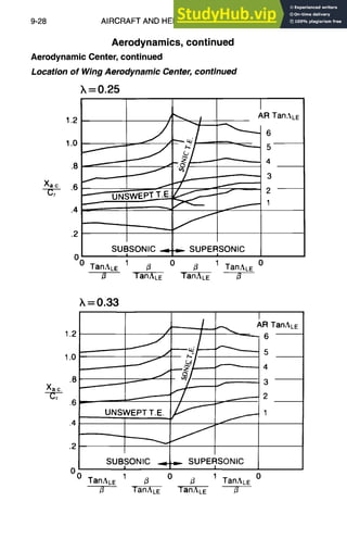
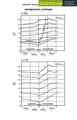
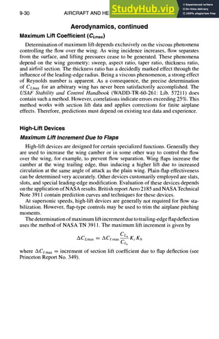
![AIRCRAFT AND HELICOPTER DESIGN 9-31
Aerodynamics, continued
AR
cLo/C,o =
oo [@)2 c As
+ 71-cosAc/2] j
where
ao = section lift-curve slope, per radian
Kb = flap span factor (see Flap Span Factor graph)
Kc = flap chord factor (see Flap Chord Factor graph)
Care should be exercised in use of all prediction techniques for ACLmax due to flap
deflection, because flap effectiveness is modified to a large extent by the ability of
the wing-leading-edge devices to maintain attached flow.
Example
Determine AfLmax due to flap deflection, with the following wing characteris-
tics.
Aspect ratio = 4.0
Section lift-curve slope = 5.73 per radian
Semichord sweep = 20 deg
Taper ratio = 0.2
4.0
CL,/Ceo = 1 = 0.6197
5.73 [(_~)2 [ 4.0 ,~1 ~
--Y- + + ~cos(20)t j
For plain flaps with 50 deg deflection, 16% chord,
ACemax = 0.80 for a typical plain flap
Inboard span, rh = 0.15 gbi = 0.22 (see Flap Span Factor graph)
Outboard span, r/o = 0.65 Kbo = 0.80 (see Flap Span Factor graph)
Kb = 0.8 -- 0.22 = 0.58
(otS)Ce = 0.5 (see Flap Chord Factor graph)
Kc = 1.1 (see Flap Chord Factor graph)
CLmax = (0.8)(0.6197)(1.1)(0.58) = 0.3163](https://image.slidesharecdn.com/aiaaaerospacedesignengineersguide-230807164453-d76eba30/85/Aiaa-Aerospace-Design-Engineers-Guide-pdf-293-320.jpg)
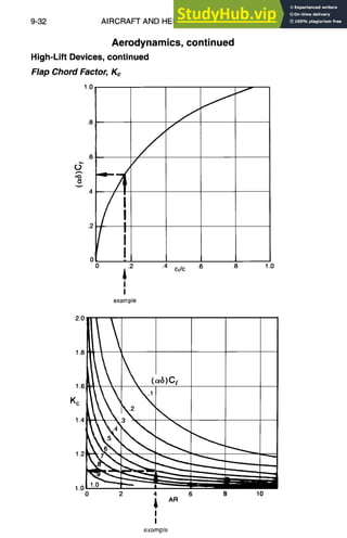
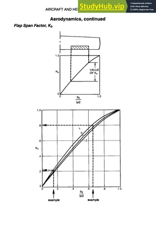
![9-34 AIRCRAFT AND HELICOPTER DESIGN
Aerodynamics, continued
High-Lift Devices,continued
Effects of Flap Deflection on Zero-Lift Angle of Attack
The set of Plain-Flap Effectiveness graphs may be used with the following
expression to obtain subsonic, plain-flap effectiveness. Correction factors for body
effect, partial span, and flap-leading-edge gap are shown.
AOtLo = (0t~/0~)COS AHLS[I -- (a + bf)l~l]
Example
Determine At~Lodue to plain-flap deflection, with the following wing charac-
teristics.
Aspect ratio = 4.0
Sweep at flap hinge line = 10 deg
Sweep at wing leading edge = 32 deg
For inboard plain flaps with 25 deg deflection, 15% flap chord,
Flap gap ratio, GAP/(f = 0.002
Inboard span, 01 = 0.15
Outboard span, qo = 0.65
Ratio of body diameter to wing span, 2Ro/b = 0.15
Approach Mach number = 0.1
,6 = ~ - M 2 = 0.995
Flap effectiveness = -0ot/0~ = 0.49 (see Plain-Flap Effectiveness graph)
Sweep factor:
-a = 0.039
(see Sweep factor graph)
b = 0.034
Fuselage factor:
(A~Lo)wB
-- 0.93 (see Wing-body graph)
(AOILo)W
Flap span factor:
SF(Ps)/SF(FS) = ~0 -- ~1 = 0.65 -- 0.15 = 0.50
(AOtLo)PS
- - -- 0.55 (see Flap span graph)
(AOtLo)FS
Flap gap factor:
(AOtL°)gap -- 0.96 (see Flap Gap graph)
(AOtLo)sealed
AotLo = (--0.49)cos(10 deg)(25)[1 - (-0.039 + 0.034(0.995))(25)]
x (0.93)(0.55)(0.96) -----6.69 deg](https://image.slidesharecdn.com/aiaaaerospacedesignengineersguide-230807164453-d76eba30/85/Aiaa-Aerospace-Design-Engineers-Guide-pdf-296-320.jpg)
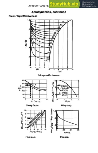
![9-36 AIRCRAFT AND HELICOPTER DESIGN
Aerodynamics, continued
High-Lift Devices, continued
Induced Drag due to Flaps Deployed
Subsonic. Trailing-edge flaps on a wing give it a camber for improving lift.
Elevons in a similar manner camber the wing, although they are utilized for control
at cruise lift values. Drag due to lift ratio can be expressed as follows.
CDi~ (l__F)(Ol~OlLo$) 2 (~--OlL°~
- - - - +F
Coi8 = 0 Ol-- OlLo -- OILo.]
where F = sin Ac/4(0.295 + 0.066ct - 0.00165ot2).
The following graph shows working plots of these relationships. Zero-lift angle
of attack with flaps deflected is obtained from the preceding section.
Supersonic. At the supersonic speeds, flaps as such are not likely to be used.
However, elevons still are required on tailless configurations for pitch control. The
subsonic data listed above may be used.
Example
Find induced-drag ratio for flaps deployed for the following wing characteristics:
angle of attack at zero lift C~Loof --6 deg and quarter-chord sweep Ac/4 : 26 deg.
For a plain flap with 25 deg deflection, and with angle of attack at zero-lift with
flaps deflected aLo~ of -10 deg, the induced-drag ratio at 10 deg angle of attack
will be as follows.
F
- - -- 0.79 (see Drag-Due-to-Lift Ratio with Flap Deflection graph)
sin Ac/4
CDi~
Coi8 = 0
- OtLo~ _ 10 - (-10) _ 1.25
ot - OtLo 10 - (-6)
F = (0.79)sin(26 deg) = 0.3463
- - -- 1.454 (see Drag-Due-to-Lift Ratio with Flap Deflection graph)](https://image.slidesharecdn.com/aiaaaerospacedesignengineersguide-230807164453-d76eba30/85/Aiaa-Aerospace-Design-Engineers-Guide-pdf-298-320.jpg)
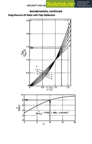
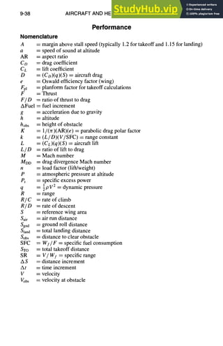
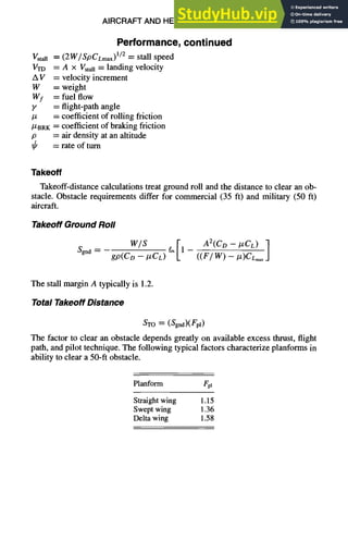
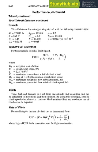
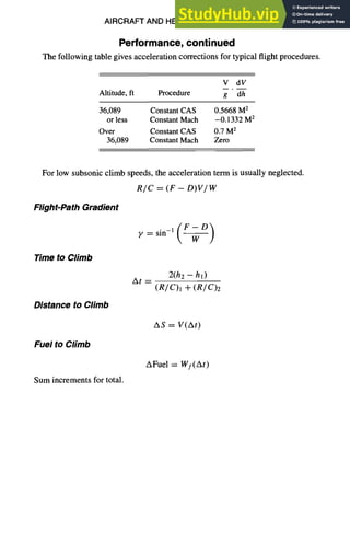
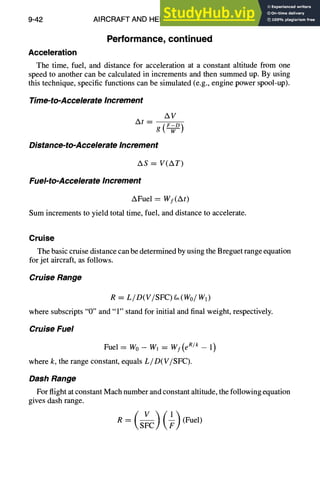
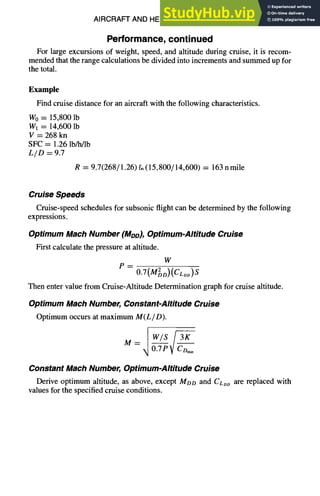
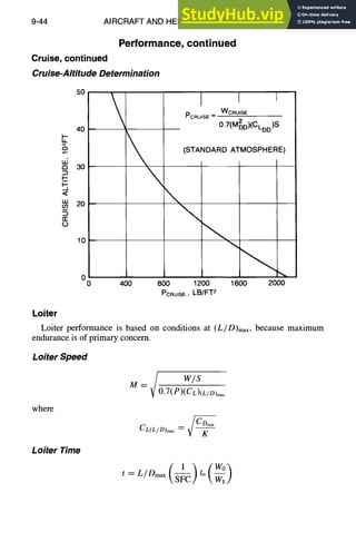
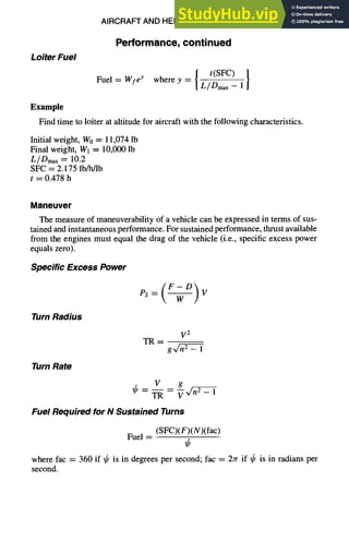
![9-46 AIRCRAFT AND HELICOPTER DESIGN
Performance, continued
Maneuver, continued
Fuel Required for N Sustained Turns, continued
Example
Determine turn radius for the following vehicle.
V = 610 fps
n=l.3g
TR = 13,923 ft
Landing
Landing distance calculations cover distance from obstacle height to touchdown
and ground roll from touchdown to a complete stop.
Approach Distance
[V2~
Sair = [ oOS2g- + hobs)(L/D)
where Vobs= speed at obstacle, VTo = speed at touchdown, hobs = obstacle height,
and L/D = lift-to-drag ratio.
Landing Ground-Roll
(W/S) ~[1- A2(CD--
#BRKCL)]
Sgnd = gp(CD -- #BRKCL) ((F---'7~ 5 ~aax
This equation, of course, also describes takeoff roll, except being positive to ac-
count for deceleration from touchdown to zero velocity.
Normally the distance would require a two-second delay to cover the time
required to achieve full braking. Commercial requirements may also dictate con-
servative factors be applied to the calculated distances.
Example
Find landing distance for an aircraft with the following characteristics.
W = 17,000 lb #BRK = 0.6
S = 262 ft2 A = 1.15
CL = 0.46 Vobs = 226 ft/s
Co =0.352 VTD =200ft/s
CLm,x= 1.44 L/D = 1.88
p = 0.0023769 lb-sZ-ft-4 hobs = 50 ft
F = 0.0
Sair= 418 ft Sgnd = 1229 ft S~and= S~ir + Sgn~= 1647 ft](https://image.slidesharecdn.com/aiaaaerospacedesignengineersguide-230807164453-d76eba30/85/Aiaa-Aerospace-Design-Engineers-Guide-pdf-308-320.jpg)
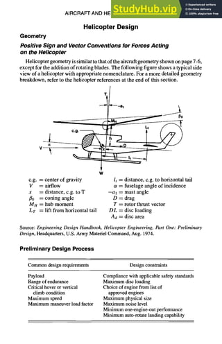
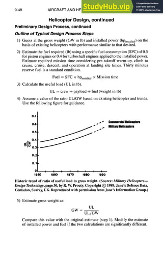
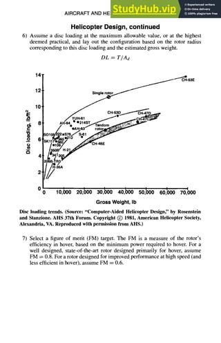
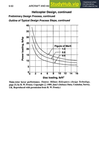
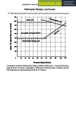
![9-52 AIRCRAFT AND HELICOPTER DESIGN
Helicopter Design, continued
PreliminaryDesignProcess,continued
Outline of Typical Design Process Steps, continued
9) Make first estimates of drag in forward flight. Estimatefe [equivalent flat plate
area, ft2(m2)] by using existing helicopters designed for similar missions as a
basis.
Parasite drag in forward flight
l
d
10,000
6,000
4,000
2,000
o~ 1,ooo ,,
e- " " , S,~34
= l
"0 ~u= recor
.2o
O~ 400 "~A341z
¢~ CH58A ~_
200
Alouette II
lOO - h
1,000 10,000 20,000 100,000
Gross Weight, Ib
Helicopter and airplane drag state of the art. (Source: "Computer-Aided Helicopter
Design," byRosenstein and Stanzione,AHS37th Forum. Copyright (~)1981,American
Helicopter Society, Alexandria, VA. Reproduced with permission from AHS.)](https://image.slidesharecdn.com/aiaaaerospacedesignengineersguide-230807164453-d76eba30/85/Aiaa-Aerospace-Design-Engineers-Guide-pdf-314-320.jpg)
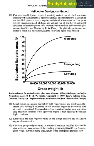
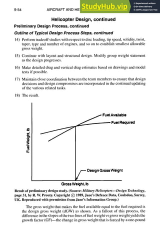
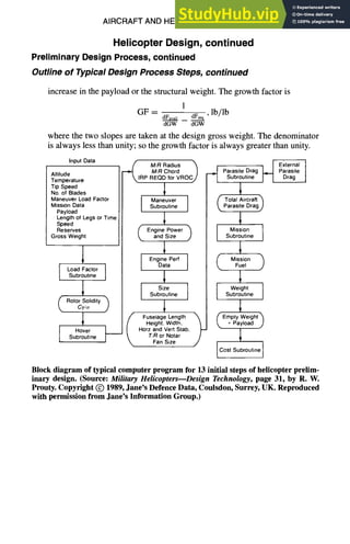
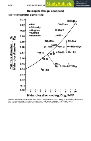
![AIRCRAFT AND HELICOPTER DESIGN 9-57
Helicopter Design, continued
Performance
2200 r
Torque limit
2000 P.~
L ~ ~ • Turboshaft engine
1800 ~'~. ~ ' ~ r r (5 • 1986 technology
.v.o
1400 " . ~ ~ ~ .
°1200
- - "A.'~~ "'%g¢~X"~" .. 7"S~ - ~ ~ )Standard
600 ous -.. ~ "...
400 -.. ~- ~.'~
"...~ 95 Fday
200
0 I i i ] i i ~ i i i i i i i i
2,000 6,000 10,000 14,000 18,000 22,000 26,000 30,000
Altitude, ft
Typical uninstalled engine ratings as a function of altitude and temperature. (Source:
Helicopter Performance, Stability, and Control, page 274, figure 4.1, by R. W. Prouty.
Copyright (~) 1995, Krieger Publishing Company, Malabar, FL. Reproduced with
permission of Krieger.)](https://image.slidesharecdn.com/aiaaaerospacedesignengineersguide-230807164453-d76eba30/85/Aiaa-Aerospace-Design-Engineers-Guide-pdf-319-320.jpg)
![9-58 AIRCRAFT AND HELICOPTER DESIGN
Helicopter Design, continued
Performance, continued
1100 - • Turboshaft Engine
,1986 technology /
1000 -
/ /
Std.Day
900 "- Max.Cont.~//.i
= 8OO6oo ~">'"]'Limit/
700- Sea-LevelStd
l< 500 5 , ~ ~ Std Day
If) I ~ ~ T. C).Limit
o 400
30O
/~/,~//.,,~ " 15,000'Std
200 ~..~//..,~" "20,O00'Std
lOO .5,ooo st.
30,000'Std
O0 260 ' 6()0 ' I0()0 ' 14'00 ' 18'00 ' 22'00
Engine Shaft Horsepower
Typicalengine fuel flowcharacteristics. (Source:Helicopter Performance, Stability, and
Control, page 276, figure 4.3, by R. W. Prouty. Copyright (~) 1995, Krieger Publishing
Company, Malabar, FL. Reproduced with permission of Krieger.)](https://image.slidesharecdn.com/aiaaaerospacedesignengineersguide-230807164453-d76eba30/85/Aiaa-Aerospace-Design-Engineers-Guide-pdf-320-320.jpg)
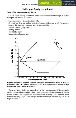
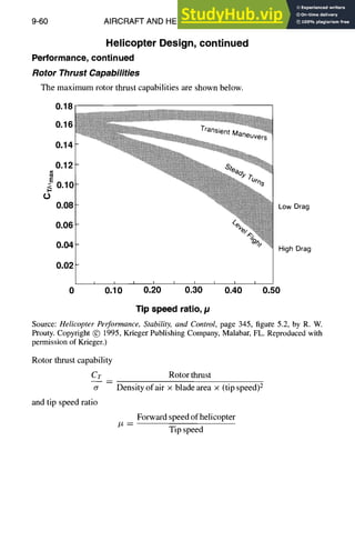
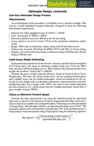

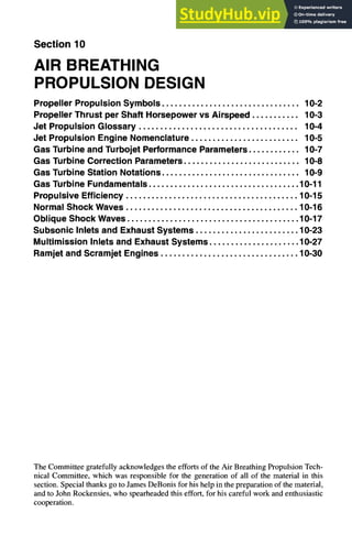

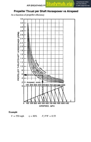


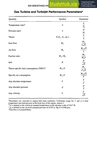
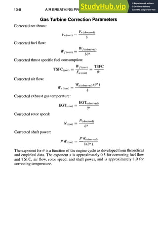
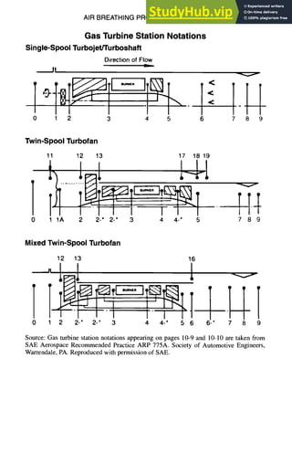
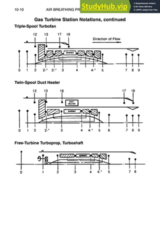
![AIR BREATHING PROPULSION DESIGN 10-11
Gas Turbine Fundamentals
The following definitions and relationships are commonly used in gas turbine
analysis; the number subscripts indicate the station at which the parameter is to
be evaluated. Values of y = 1.4, Cp = 0.241 and cv = 0.173 for air at standard
conditions can be used in the equations that follow to yield approximate results. For
more exact results, the work of compression and expansion of air can be determined
by using tables that reference the properties of air at different temperatures and
pressures and take into account variations in y and cp.
Compressor power:
Pc = W2cpc(Tt3 - Tt2) Btu/s
Compressor efficiency:
Tt3 - Tt2
Turbine power:
etur = W4cptur (Tt4 - Tt5) Btu/s
Turbine efficiency:
Power balance:
~tur
Tt4 - Tt5
Tt4[1-(pts/Pt4) ~ ]
Pm 71- W2cpc(Tt3 - Tt2) = W4cptur(Tt4 - Tt5) Btu/s
where Pm= mechanical drive output power required to drive the fan of a turbofan
engine or the power to drive the propeller shaft of a turbo-prop engine. Also
included in this category are aircraft/engine accessories (i.e., fuel pumps, fuel
controls, oil pumps, generators, hydraulic pumps).
In the analysis of an engine, the requirement of airflow continuity through the
engine must be satisfied. Small pressure losses occur in the combustion and exhaust
systems and have to be minimized by careful design of these systems. The amount
of total pressure loss is characterized by the ratio of total pressure at combustion
chamber discharge Pt4 to the total pressure at the combustion chamber entrance
Pt3, and is equal topt4/Pt3. Typical values of total pressure loss coefficients are
between 0.93 and 0.98. Losses in the exhaust system will be minimized if the
tailpipe is made as short as possible, which will reduce wall friction losses.
The gas turbinefundamentalsmaterialappearingon pages 10-11-10-14 is from the General
ElectricAircraftPropulsionDataBook,AEG.215.4168(15 m), pages 3-7; reference data is
taken from Jet Engines:Fundamentalsof Theory,Design,and Operations,pages 128 and
129,by K. Hunecke.Copyright @ 1997,MotorbooksInternational,St. Paul, MN. Reprinted
with permission of GE and Motorbooks.](https://image.slidesharecdn.com/aiaaaerospacedesignengineersguide-230807164453-d76eba30/85/Aiaa-Aerospace-Design-Engineers-Guide-pdf-335-320.jpg)
![10-12 AIR BREATHING PROPULSION DESIGN
Gas Turbine Fundamentals, continued
Allowance also must be made for the combustion efficiency of the burner. In
general, injected fuel does not burn completely and produces less heat than would
be possible theoretically. The degree of actual fuel usage is characterized by a
combustion efficiency factor 0b giving the amount of heat released by combustion
to the heat theoretically available in the fuel. Modem combustion chambers achieve
efficiencies between 0.90 and 0.98.
Note that in the following equations subscripts are shown as station 9 indicating a
convergent-divergent nozzle. For a convergent nozzle the subscript would indicate
station 8.
Jet velocity:
V 9 = Cv~ZgJcpTt9 [1 - (p9/Pt9) y-I/e]
where Cv is the coefficient of velocity that is equal to the nozzle efficiency (qnoz)1/2.
Thrust (gross):
W~
Fg = ~V9q-A9(P9-Po)
g
The pressure-area product here is zero if the nozzle allows complete expansion,
that is, if P9 = Po.
In the inlet system the following equations apply:
Tt___~2
= Tto = 1 + ~' - 1M2
To To 2
Pt2po-- --PtoPt2
Pt° -- Pt2 II -k- Y - IM21
Pro 2
where Pt2/Pto is the total pressure recovery of the inlet system.](https://image.slidesharecdn.com/aiaaaerospacedesignengineersguide-230807164453-d76eba30/85/Aiaa-Aerospace-Design-Engineers-Guide-pdf-336-320.jpg)
![AIR BREATHING PROPULSION DESIGN 10-13
Gas Turbine Fundamentals, continued
Propulsion of a jet aircraft is accomplished by the principle of reaction, where a
gas exhausting at a high velocity through a nozzle generates a force in the opposite
direction, which is termed thrust. The amount of thrust depends on the mass of
the airflow passing through the engine and the exhaust velocity, the product of
which (Wig × V) is termed momentum. Changes in momentum per unit time
(conservation of momentum theorem) result in a force being generated that is the
basis for jet propulsion. Consider an engine installed in a nacelle as indicated in
the following figure.
V FIo~ velocilv J ................... -7
,.x A~¢,~ " / /
p Pressure /" Dra~ /
----- Control / .... ~ / /
, / " ~ / - P',- ~Mnbzent
vommc /" ~ 1 .,
lh-essure p~j , " -- i
Pressure force I ~ ;
P0 x A t gA~ 'l]qrttst @
Source: Jet Engines: Fundamentals of Theory, Design, and Operations, page 33, by
K. Hunecke. Copyright @ 1997, Motorbooks International, St. Paul, MN. Reprinted by
permission of Motorbooks.
This figure shows a control volume that allows flow to pass from open boundaries
from engine station 1-9 but does not transfer momentum effects across solid
boundaries that make up the engine casing.
Calculation of the engine thrust can be made knowing the boundary conditions at
the inlet and exit of the engine. The conditions internal to the engine are represented
by Fret,a resultant force where the propulsive thrust can be taken as the integral over
those surfaces and components of the engine where thrust is most directly apparent,
or chiefly exerted (e.g., inlet, compressor, diffuser, burner, turbine, nozzle, and the
surfaces inside and outside of the engine).
Applying the conservation of momentum theorem to the internal flow between
stations 1 and 9 gives
poA1 + /~nt -- p9A9 = W9 V9 - W~Iv1
g g
Fint ~ W9V9 7t- A9(P9 - P0) - W--~Iv1+ po(A9 - A1)
g g](https://image.slidesharecdn.com/aiaaaerospacedesignengineersguide-230807164453-d76eba30/85/Aiaa-Aerospace-Design-Engineers-Guide-pdf-337-320.jpg)
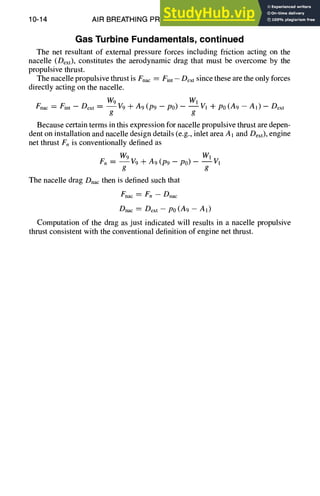
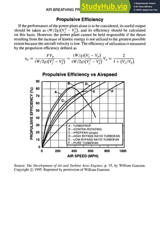
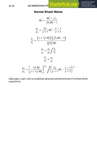
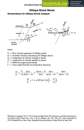
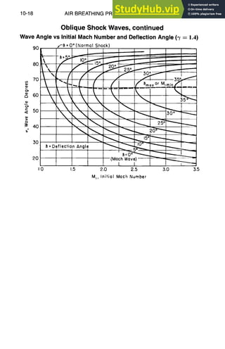
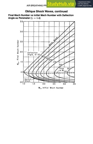
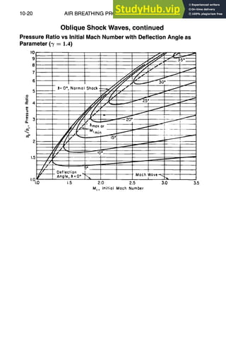
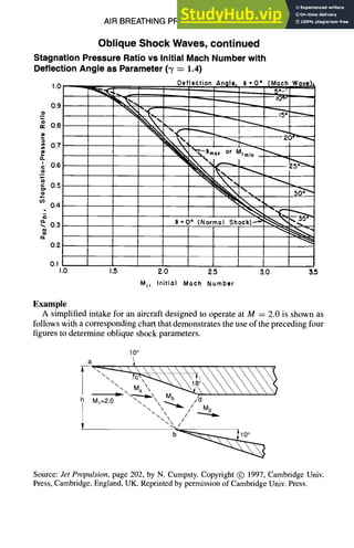
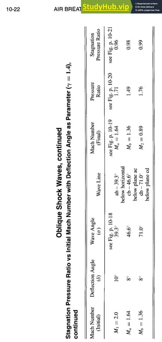
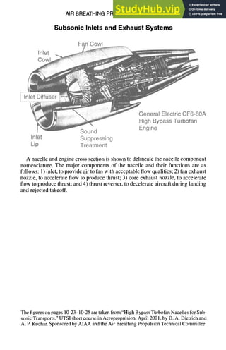
![10-24 AIR BREATHING PROPULSION DESIGN
Subsonic Inlets and Exhaust Systems, continued
Inlet and Fan Cowl Component Design Parameters
d
I- Lmax D'lq Lfc
~ lr!ax
(Amax)
~~r~ e~BOattail
rhl
(ihl)r]h
(Ath2(~cc~iff)Engine
Centerline }ne
1"~ kinlet=I
The following are the most significant geometric parameters and their major
influence factors used in describing a particular inlet design. These parameters have
been determined from the results of an experimental database, flowfield analysis,
and wind tunnel testing.
rh]/rth : the low speed angle of attack and crosswind performance
rh]/rmax : high speed drag and engine-out cowl drag
rfa. tip/rth : inlet diffuser recovery and influence on distortion
Typical Values for Inlet Design Parameters
Parameter Typical values
Maximum Mth 0.70-0.77
Ld/rff 0.56-0.90
rh]/rth 1.11--1.20
rhl/ rmax 0.75--0.86
Lmax/rmax 0.80-1.30
Typical values are shown for throat Mach number at nominal maximum corrected
flow, rhl/rth (internal lip contraction), rh]/rma× (forebody diameter ratio), and dif-
fuser area ratio Afa, tip/Ath. Specific installation values depend on particular re-
quirements, but the values shown generally reflect the following:
1)Design throat Mach number Mth is moderately high to near choking, to reduce
nacelle size, assuming moderate-to-high cruse flight speed.
2) There are typical takeoff climb incidence and crosswind requirements, with
some tendency toward increasing the ratio rhl/rth, which indicates a thicker lip,
proceeding from top to bottom around the periphery.](https://image.slidesharecdn.com/aiaaaerospacedesignengineersguide-230807164453-d76eba30/85/Aiaa-Aerospace-Design-Engineers-Guide-pdf-348-320.jpg)
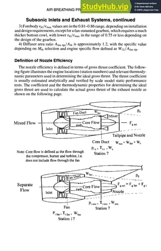
![10-26 AIR BREATHING PROPULSION DESIGN
Subsonic Inlets and Exhaust Systems, continued
Definition of Nozzle Efficiency, continued
Fgact
Cfg -- Finoz -- Nozzle gross thrust coefficient
where
Fgact = nozzle actual gross thrust
Finoz = nozzle ideal gross thrust
= (Wnoz/g) V~noz, for mixed flow
: (Wfan/g) V/fan -']- (We~g) gic, for separate flow
Ideal velocity, where flow is completely expanded to ambient pressure at the
gas stream total temperature and total pressure, is represented by the following:
V/'noz = f (Ptnoz/P0, Ttnoz)
V/fan = f(Ptfan/PO, Ttfan)
V/c = f (Ptc/PO, Tt~)
Definition of Engine Net Thrust Fnand Net Propulsive Force NPF
F. = Fgact -- Dr = engine net thrust (provided by the engine manufacturer)
where Dr = (Wo/g)Vo = ram drag and Fgact = engine actual gross thrust.
NPF = Fn - Dcowl - Dinlet - Dinter
where
Dcowl = cowl drag
Dspillage = inlet spillage drag
Dinte r = interference drag
which are determined by the aircraft manufacturer from scale model wind tunnel
tests.](https://image.slidesharecdn.com/aiaaaerospacedesignengineersguide-230807164453-d76eba30/85/Aiaa-Aerospace-Design-Engineers-Guide-pdf-350-320.jpg)
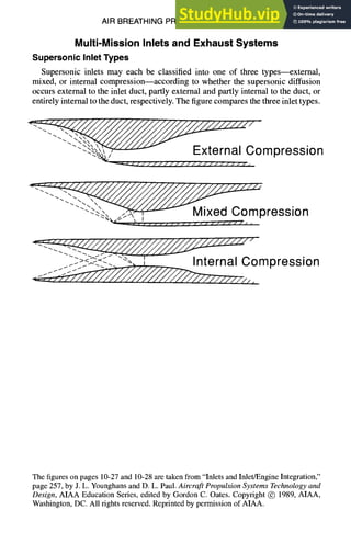
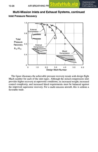
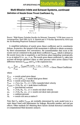

![10-32 AIR BREATHING PROPULSION DESIGN
Ramjet and Scramjet Engines, continued
The RamjetEngine,continued
Jet Engine Operational Envelopes
200
150
ALTITUDE,
1000 FT
100
50
0
0 2 4 6 8 10
FLIGHT MACH NUMBER
Source: "Advanced Ramjet-Scramjet Technology,"UTSI Short Course in Aeropropulsion,
Nov. 1981, by A. N. Thomas, Jr. Sponsored by AIAA and the Air Breathing Propulsion
Technical Committee.
Ideal Performance of a Ramjet
The ideal performance of a ramjet is characterized by a cycle shown on a tem-
perature vs entropy diagram (see page 10-36), where compression in the inlet
and expansion in the nozzle are isentropic processes (constant entropy), and the
heat added in the combustion chamber is a thermodynamically reversible process.
Therefore these processes do not take into account any nonideal conditions where
performance in the cycle is degraded because of total pressure losses due to shocks,
friction, heat due to friction, and mass diffusion.
The ideal engine thrust is
Fn = wa [(1 ~- f) gj -- gp]
g
The ramjet ideal performance text appearing on pages 10-32 and 10-33 is based on
Mechanics and Thermodynamics ofPropulsion, 2nd Edition, pages 151 and 152,by E Hill
and C. Peterson, Copyright @ 1992, Addison-Wesley, Reading, MA. Reprinted by permis-
sion of Pearson Education, Inc.](https://image.slidesharecdn.com/aiaaaerospacedesignengineersguide-230807164453-d76eba30/85/Aiaa-Aerospace-Design-Engineers-Guide-pdf-356-320.jpg)
![AIR BREATHING PROPULSION DESIGN
Ramjet and Scramjet Engines, continued
The specific thrust (thrust per pound of airflow per second) is
_,
where
F./ Wa= net thrust/lb airflow/s
Tt4 = total combustion temperature, °R
To = free stream static temperature, °R
The thrust specific fuel consumption, TSFC, is
TSFC -- WI _ f x 3600
Fn F./Wo
where the fuel-air ratio f is defined as
f =
(~4/~0) -- ]
(Q/cp~,o) - (T,4/v,0)
10-33
Note that r/b is the combustion efficiency and qb Q is the actual heat release per
unit weight of fuel.](https://image.slidesharecdn.com/aiaaaerospacedesignengineersguide-230807164453-d76eba30/85/Aiaa-Aerospace-Design-Engineers-Guide-pdf-357-320.jpg)
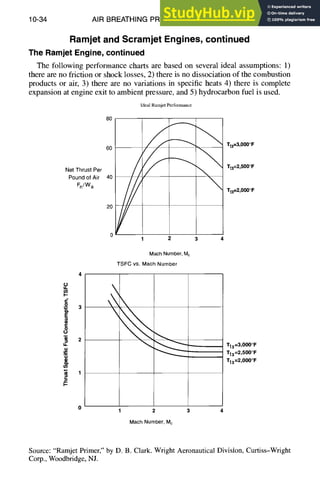
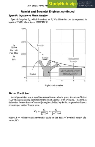
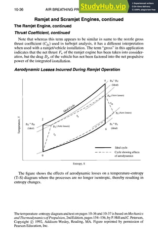
![AIR BREATHING PROPULSION DESIGN 10-37
Ramjet and Scramjet Engines, continued
Losses in the ramjet engine are characterized by total pressure losses due to
shocks, friction, heat and mass diffusion, etc. The total pressure loss ratios for
inlet (diffuser), combustor (burner), nozzle and engine are
rd
rb
r n
Pt6
Pro
Pt2
Pto
Pt4
Pt2
Pt6
Pt4
-- r d rbrn
The thrust per unit air flow rate (nonideal) is
1
Fn _ 1 [(1 + f) Vj - Vp] + Waa(P6 -- PO)A6
Wa g
or
where
Fn (1-l-f) /2yRTt4(m-1) M p6A6 (1_ p~)
- V y,/V-o +
(y l)
m=(I+Y--IM2) (rdrbrnp°)
P6/
The thrust specific fuel consumption is
f x 3600
TSFC --
F.IW~](https://image.slidesharecdn.com/aiaaaerospacedesignengineersguide-230807164453-d76eba30/85/Aiaa-Aerospace-Design-Engineers-Guide-pdf-361-320.jpg)
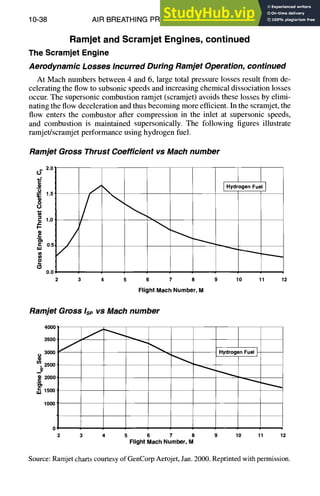

![SPACECRAFT AND LAUNCH VEHICLE DESIGN 11-3
Spacecraft General Information, continued
Spacecraft BlockDiagram
Spacecraft I
I Payload ]l ,[ Spacecraftbus ]
J Communications
Antennas
Transponder
Meteorology
Veryhigh
resolution
radiometer
Earth resources
Multispectral
scanner
Scientific
Surveillance
Attitude control
Sensors
Torquers
Angularmomentum
storage
Propulsion
Orbit injection(solid
and liquid)
Orbit correction
(liquid)
Torquer (liquid)
Electricpower
Solarcells
Batteries
Powercontrol
electronics
Thermalcontrol
Coatings
Insulation
Activecontrol
_~ Stmcture
Mainstructure
Deployment
mechanisms
Telemetry and command
Encoder
Decoder
Source: Designof Geosynchronous, Spacecraft,page 3, figure 1.2, by B. N. Agrawal.
Copyright (~) 1986, Prentice-Hall, Englewood Cliffs, NJ. Reprinted by permission of
Prentice-Hall, Inc.](https://image.slidesharecdn.com/aiaaaerospacedesignengineersguide-230807164453-d76eba30/85/Aiaa-Aerospace-Design-Engineers-Guide-pdf-365-320.jpg)
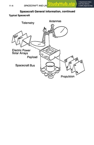
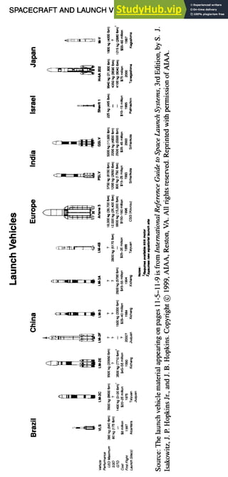

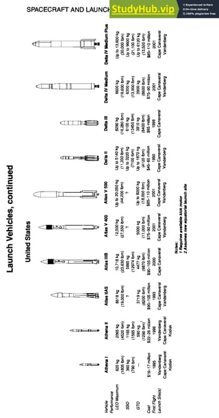
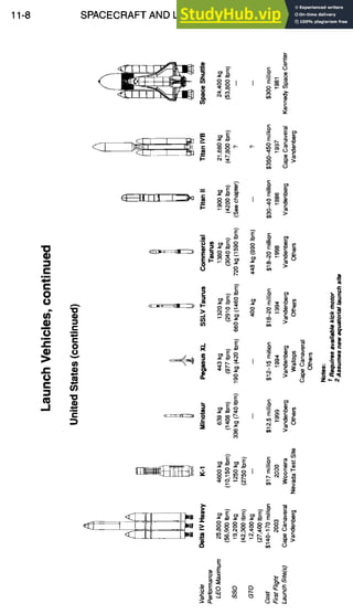
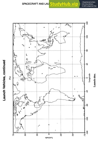
![11-10 SPACECRAFT AND LAUNCH VEHICLE DESIGN
Launch Vehicles, continued
Space Shuttle Launch Configuration
(2) solid rocket
External / boosters (SRB) ~ ~-
Cargo bay envelope<.,,..,.,,_
~" (16.03'trn)--'~ / ~
Orbit, ~f~.~
100 X103
40 X 103
]0
30 ~0
~20
;0
c &
10 tO
--•lntegral
OMS as early as possible.
,
~T- First OMS
i. Secon O S
"'~' N, ~ ~ "',-,,,,,,dr.--'T-Third
OMS
'~'-~ k ~ kitadded
•
"-.,
0
100 200 300 400 500 600
Circular orbit altitude (nmi)
I I I I I I
200 400 600 800 1000 t 200
• Shuttle performance is a function of program variables
(launch date. engine Thrust, individual orbiler weTghl,
etc.) and must be determined on a caseby casebasis
• Cargo weight includes all payloaOitems ano oayload
support services.
• Data shown for 28.5; inclination only.
• Shadedareasrepresent primary regionsaffec:ed bv
-- program variables. Payloadsrequiring performance
in these regions should verify capability w,tn JSC
Circular orbit altitude (kin)
Near-termSpaceShuttlecargoweightvscircularorbitalaltitude-KSClaunch
700 800](https://image.slidesharecdn.com/aiaaaerospacedesignengineersguide-230807164453-d76eba30/85/Aiaa-Aerospace-Design-Engineers-Guide-pdf-372-320.jpg)
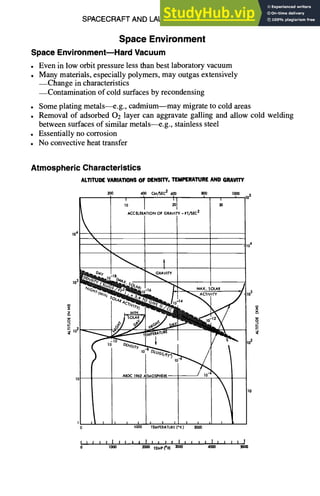
![11-12 SPACECRAFT AND LAUNCH VEHICLE DESIGN
Space Environment, continued
Space Environment--Radiation
• Cosmic Rays
--Infrequent, highly energetic
--Shielding impractical
--Total dose not a problem
--Single event upset can be serious
• Solar Flare
--Usually not serious for electronics
--Human crew requires 2-4 g]cm2 shielding for average event
--Infrequent major event may require 40 g/cm2 for crew
• Radiation Belts
--Charged particles trapped by planetary magnetic field
--Earth's Van Allen belts a major problem to both electronics and crew
--Jupiter radiation environment very severe
Natural Radiation Environment for Various Orbits
lot~
106
ELECTRONS 0
PROTONS 0
. . . . ELLIPTICAL ORBIT SELECTED FOR
HIGH RADIATION EXPOSURE
180 x 10,000 nmi 0° INCLINATION
10TM ~ - GEOSTATIONARY ORBIT - EQUATORIAL
LOW EARTH ORBIT UP TO 400 nmi
%' ANY INCLINATION
ELECTRON DATA -- NASA MODEL AEI-7 Hi
Z • PROTON DATA -- NASA MODEL AP-8
10I1 ~.-.~
DE
1010 el ",.
>. ,.
(3 " ~'
z !'
109 ,,.e
%,%-.,
%
-.J 108 "-. ~ "~.
107
p+ ~ ~.. ~ p+
1 2 3 4 5 6
50 100 150 200 250 300
PARTICLE ENERGY (E) MeV](https://image.slidesharecdn.com/aiaaaerospacedesignengineersguide-230807164453-d76eba30/85/Aiaa-Aerospace-Design-Engineers-Guide-pdf-374-320.jpg)

![1 1-14 SPACECRAFT AND LAUNCH VEHICLE DESIGN
Space Environment, continued
Space Environment--Oxygen Atom FluxVariationwith Altitude
a
i-.
.J
<~
9OO
800
700
60(]
sooI
400
•
•%
300
1012 1016
SUNSPOT MAXIMUM
~ STANDARD ATMOSPHERE
- ~ SUNSPOT MINIMUM
L
10 I"~ 1014 10is
1017 10TM 1019
OXYGEN ATOM FLUX (m -2 sec-l), v = 8 kin/tee
Space Environment--Meteoroid/Debris
Meteoroid
• Large particles very rare
• Most damage pitting/sandblasting
• Near comet environment can be hazardous
• Planetary bodies increase concentration but also shield
Protection
• "Whipple meteor bumper" very effective for high velocity particles
• Large slow particles very difficult
Debris
• Major, growing problem in lowEarth orbit
• Launch debris, explosions, ASAT tests
• Armoring imposes tremendous mass penalty](https://image.slidesharecdn.com/aiaaaerospacedesignengineersguide-230807164453-d76eba30/85/Aiaa-Aerospace-Design-Engineers-Guide-pdf-376-320.jpg)
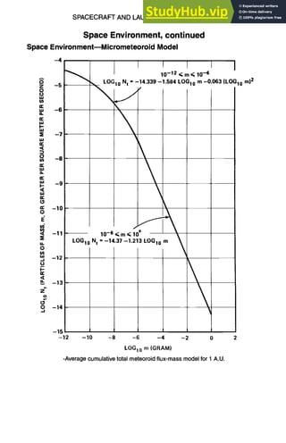
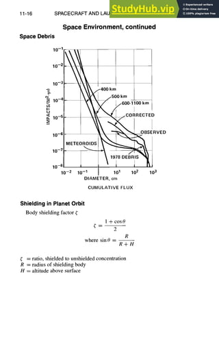
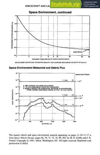
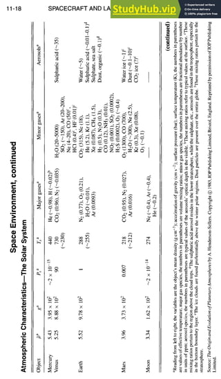
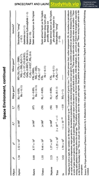
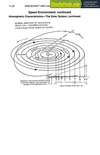
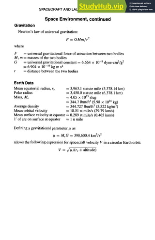
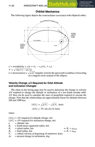
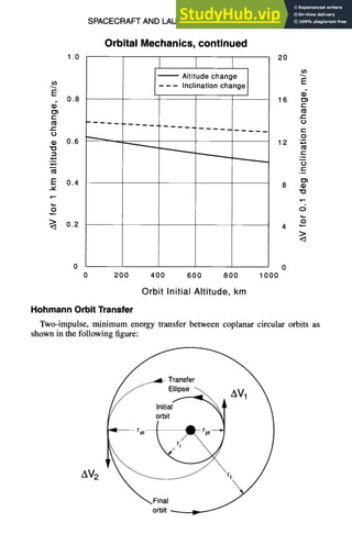
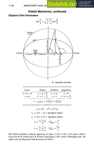
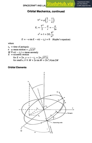
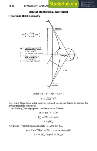
![SPACECRAFT AND LAUNCH VEHICLE DESIGN 11-27
Orbital Mechanics, continued
This is the basis for "gravity assist" maneuvers.
e= l+(rpV2/Iz)=~/[l+(~V~/tz) 2]
= rp~[1 + (2#/rpV2~)]
(rp/~) = (--Iz/~V~) = ~ll + (Iz/flV2) 2}
Satellite Lifetime vs Altitude
F=ma
Fd = Msc--
AV _ O'CdV2Af
At 2
.'. Satellite life = At _
MscA V
CdAfpV 2
seconds
where
Fd
Msc =
AV=
At =
p =
C d =
V =
Af =
Cb =
atmospheric drag force, N
spacecraft mass, kg
change in velocity, km/s
time increment (satellite lifetime), s
atmospheric density, kg/m3
drag coefficient, assumed to be 2.0
orbital velocity, km/s
projected area of spacecraft normal to velocity vector, m 2
ballistic coefficient = BC = Msc/CdAf, kg/m 2
The following chart shows the approximate lifetime of a satellite, as determined
by the atmospheric drag. End of life is defined as loss of 50 km of altitude; no
additional propulsion is assumed.](https://image.slidesharecdn.com/aiaaaerospacedesignengineersguide-230807164453-d76eba30/85/Aiaa-Aerospace-Design-Engineers-Guide-pdf-389-320.jpg)
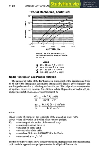
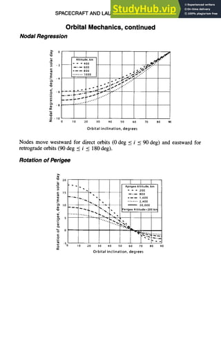
![11-30 SPACECRAFT AND LAUNCH VEHICLE DESIGN
Orbital Mechanics, continued
Inclination for Sun-Synchronous Orbits
The oblateness of Earth can cause fairly large secular changes in the location of
the longitude of the ascending node. Solving for the inclination i in the previous
equation for df2/dt results in
["2a2-~n~df2/dt
e2 _]
/-----zr-acos[ (1 +e 2)
With df2/dt set to the rotational rate of the Earth about the sun, about 1 deg/day,
the following chart results, which shows the approximate inclination of sun-
synchronous, circular, or elliptical orbits:
102 ecentricity, e
0 (circular)
100 -- 0.2
0.4
0.6
................ 0.8
98
O
- ~
~ 96 ~'
94 ~.~.~-~""
92
90
0
, ..... J . . . . . . . . . . . . . ~ ......... ,. -.-
200 400 600 800 1000 1200 1400
Perigee Altitude (km)](https://image.slidesharecdn.com/aiaaaerospacedesignengineersguide-230807164453-d76eba30/85/Aiaa-Aerospace-Design-Engineers-Guide-pdf-392-320.jpg)
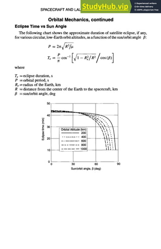
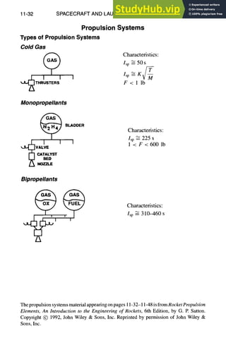
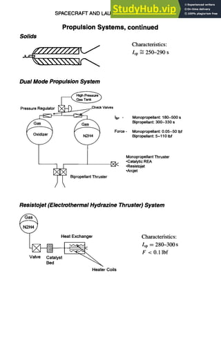
![11-34 SPACECRAFT AND LAUNCH VEHICLE DESIGN
Propulsion Systems, continued
Summaryof Key Equationsfor IdealRockets
Atmosphere@
P3
Chamber ~ k't
01, Pl, A~, Tl
llll
vl at, pt, At p2, P2, Az, T2
Nozzle Nozzle
throat exit
o
Note: Four subscripts are used above (1, 2, 3, t). They are shown in circles and
refer to the specific locations. Thus, Pl is the chamber pressure, P2 is the nozzle
exit pressure, P3 is the external fluid of atmospheric pressure, and Pt is the nozzle
throat pressure. Ta is the combustion chamber absolute temperature.
Parameter Equations
Average exhaust velocity,
v2 (m/s or ft/s)
(assume that Vl = O)
Effective exhaust velocity,
c (m/s or ft/s)
Thrust, F (N or lbf)
Characteristic exhaust
velocity, c* (m/s or ft/s)
v2 = c - (P2 - p3)A2/th
When P2 : P3, v2 : c
v2 = ~/[2k / (k - 1)]RT1 [1 - (pz/ pl) (k-1)/k]
= ~/2(hl -- h2)
c = C*CF = F/rh = Ispgo
c : v2 + (P2 -- p3)A2//n
F = crn = cmp/tb
F = CFP1At
F = rhv2 + (P2 -- p3)A2
F :/nlsp/go
c* = C/CF = piAt/rh
C* =
k~/[2/(k + 1)](k+l)(k l)
C* : Ispgo/ C F
(continued)](https://image.slidesharecdn.com/aiaaaerospacedesignengineersguide-230807164453-d76eba30/85/Aiaa-Aerospace-Design-Engineers-Guide-pdf-396-320.jpg)
![SPACECRAFT AND LAUNCH VEHICLE DESIGN
Propulsion Systems, continued
11-35
Parameter Equations
Thrust coefficient, C F
(dimensionless)
C F = c/c* = F/(plAt)
f 2k2 [ 2 (k+l)/(k-l) r (p2) (k-Wk]
= ) j
P2 -- P3 A2
4 - -
Pl At
Atvt
Mass flow rate, rn rh -- -- -- plA1/c*
(kg/s or lb/s) Vt
= A,pl k~/[2/(k + 1)](k+l)/(k-l)
f,b
Total impulse, It It = Fdt
[N-s or lbf-s] =Ftb (F constant over tb)
Specific impulse, Isp Isp = c/go = C*CF/go
[N-s/(kg x 9.8066 Isp = F/mgo = F/w
m/s2) or lbf-s/lbm Isp = v2/go + (P2 -- p3)A2/(rngo)
or s] Isp = It/(mego) = It/w p
Propellant mass fraction
(dimensionless) ( ----"mp/mo -- mo --
m y
m0
(=l-MR
Mass ratio of vehicle or
stage, MR (dimensionless)
Vehicle velocity increase in
gravity free vacuum, Av
(m/s or ft/s)
(assume that v0 = 0)
Propellant mass flow rate, rh
(kg/s or lb/s)
MR- m f _ mo -m a
mo mo
= mi/(m I + rap)
mo = mf --[-mp
Av = -c &MR = +c &m0
mf
= c ~ mo/(mo -- mp)
= c ~,(mp + mf)/mf
= Isago ~ MR
~t = Av/V = Alvl/V1
= Atvt/Vt = A2Vz/V2
rh = F/c = plAt~c*
• , /[2/(k + 1)](k+l)/(k-l)
th : mp/t b
(continued)](https://image.slidesharecdn.com/aiaaaerospacedesignengineersguide-230807164453-d76eba30/85/Aiaa-Aerospace-Design-Engineers-Guide-pdf-397-320.jpg)
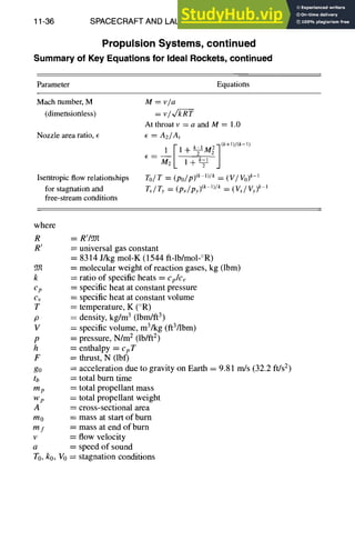
![SPACECRAFT AND LAUNCH VEHICLE DESIGN 11-37
Propulsion Systems, continued
Summary of Key Equations for Solid Rocket Motors
Mass flow rate, kg/s (lbm/s):
rh = Abrpb
d / k [ 2 "~(k+l)/(k-1)
= ~(plV1) + AtPl~/-~l~-~---~)
Burn rate r, in./s:
Propellant mass mp, kg (Ibm):
Assuming:
r -=ap'~
mp=f rndt=pbf Abrdt
d / k [ 2 ,~(k+l)/(~-l)
-~(p, Vc) <<AtPlV--~I ~-~--~)
(Rate of change of gas mass in motor cavity is small relative to mass flow through
the nozzle.)
Then,
Ab . ['Ratio of burning area-]
At -- /~ Lto nozzle throat area J
p~l-n)x/k[2/(k + 1)](k+l)/(k-l)
pba~--~l
It follows:
Pl = [Kpbac*] 1~(l-n)
where
Ao = burn area of propellant grain
Pa = solid propellant density prior to motor start
V1 = combustion chamber gas volume
a = burn rate coefficient
n = burn rate exponent](https://image.slidesharecdn.com/aiaaaerospacedesignengineersguide-230807164453-d76eba30/85/Aiaa-Aerospace-Design-Engineers-Guide-pdf-399-320.jpg)
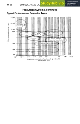
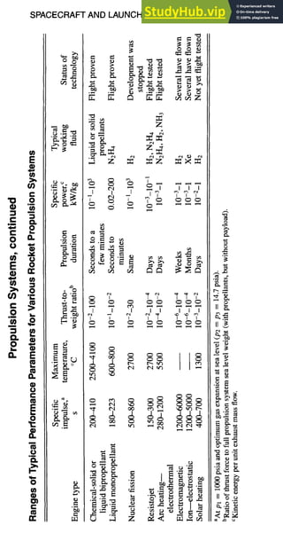
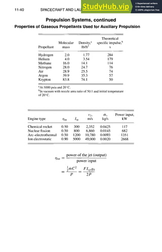
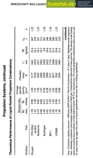
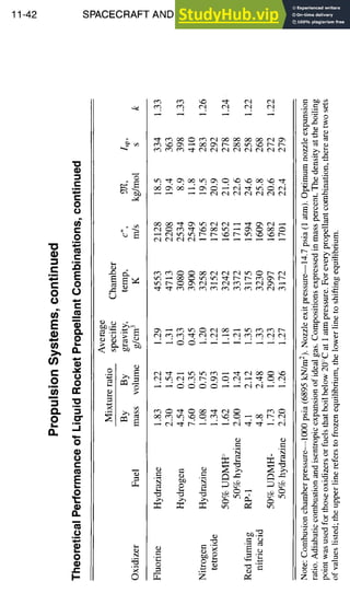
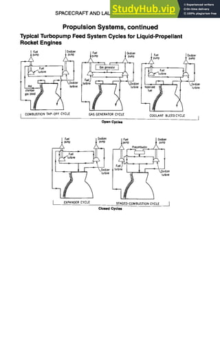
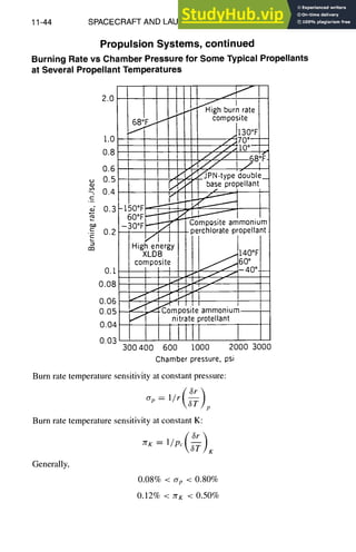
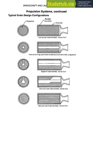
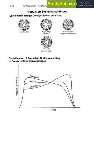

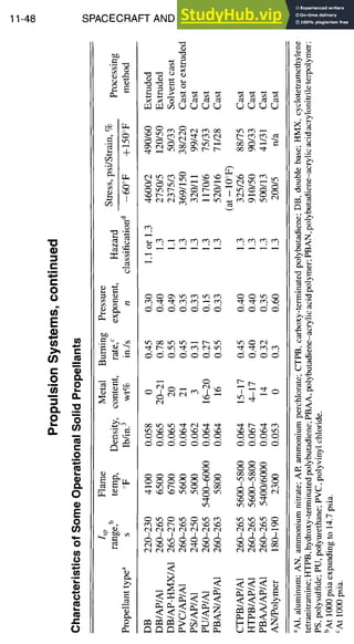
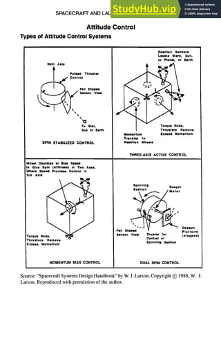
![11-50 SPACECRAFT AND LAUNCH VEHICLE DESIGN
Attitude Control, continued
Types
ofAttitude
Control
Systems,
continued
Typical
Method accuracy Remarks
Spin 0.1 dog Passive, simple; single axis
stabilized inertial; low cost
Gravity 1-3 dog Passive, simple; central body
gradient oriented; low cost
Jets 0.1 dog Consumables; fast; high cost
Magnetic 1 dog Near Earth; slow; low weight,
low cost
Reaction 0.01 dog Internal torque, requires
wheels other momentum control;
high power, cost
Coordinate
Frames
The attitude of a satellite defines the relation between a reference coordinate
frame and a satellite body-fixed coordinate frame.
ZR ZB ZS
ro~~j Tatt
]Tsen
XR XB XS
Measurements of reference vectors (e.g., sun, stars, local vertical) made in the
sensor frame are used to compute the attitude matrix Tatt. Tatt is usually parame-
terized in Euler angles for analysis or Euler symmetric parameters (quaternions)
for numerical computations.
The choice of an Euler angle sequence for the transformation Tatt is dependent on
the application, such as inertially stabilized, spin stabilized, or vertically stabilized.
Proper choice of the Euler angle sequence will simplify the formulation. A typical
Euler angle sequence (0, q~, gr) is shown in the following figure.
The attitude control material appearing on pages 11-50-11-54 is from SpaceVehicleDesign,
pages 282, 283, 288, 289, by M. D. Griffin and J. R. French. Copyright @ 1991, AIAA,
Washington, DC. All rights reserved. Reprinted with permission of AIAA.](https://image.slidesharecdn.com/aiaaaerospacedesignengineersguide-230807164453-d76eba30/85/Aiaa-Aerospace-Design-Engineers-Guide-pdf-412-320.jpg)

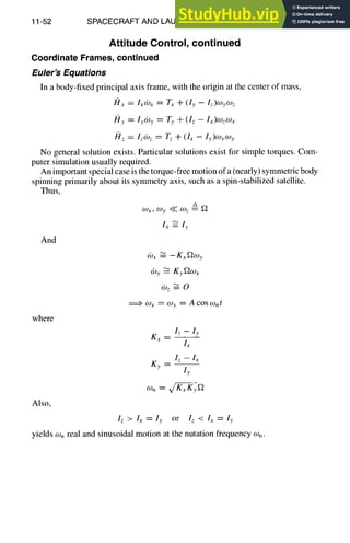
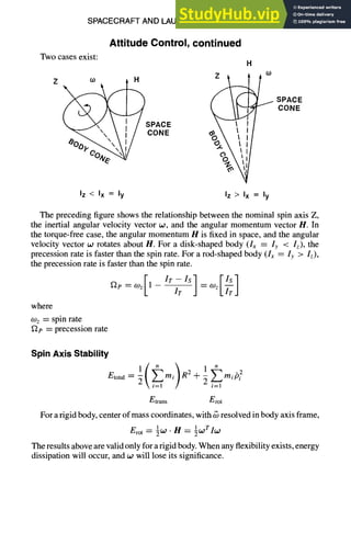

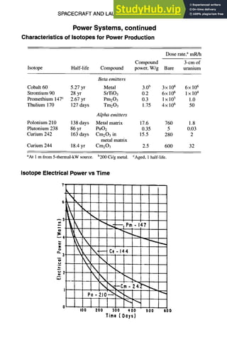


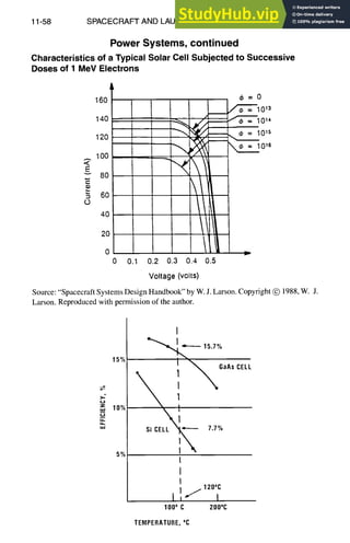
![SPACECRAFT AND LAUNCH VEHICLE DESIGN 11-59
Power Systems, continued
Nadir Pointed Spacecraft with a Flat, Rooftop Solar Array
O FIXED, 0° CANT
[] FIXED, 15°CANT
,& FIXED, 30" CANT
O FIXED, 45° CANT
FLAT
PLAT~
22
1~=/iNGLE BErWI-:ENTHEECLIPTICPLANEANO THEORBITPI.,~E
t" CJ~ ANG~
Eclipse Time vs Beta
40
A 3O
_=
E
,?,
10
',",,7 ,
,~0
0
0 30 60 90
s~ (d~)
Source: "Spacecraft Systems Design Handbook" by W. J. Larson. Copyright@ 1988, W. J.
Larson. Reproduced with permission of the author.
Te = (P/180), cos -] [(1 -- R2e/R2)0"5/cos(fl)]
P = 2 • 7~ • [R3/398,600.8]°'5/60
where
Te = eclipse time, min
P = orbital period, min
Re = radius of Earth, 6378.135 km
R = distance from the center of Earth to the s/c, km
fl = sun/orbit angle, deg](https://image.slidesharecdn.com/aiaaaerospacedesignengineersguide-230807164453-d76eba30/85/Aiaa-Aerospace-Design-Engineers-Guide-pdf-421-320.jpg)
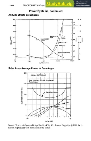
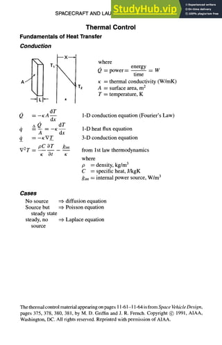
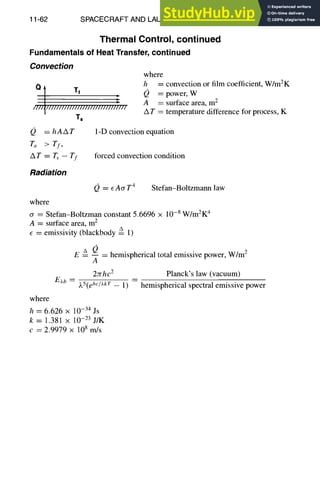
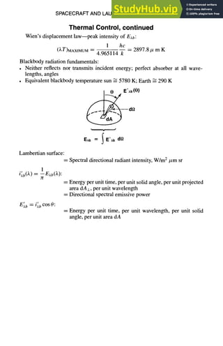
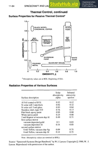
![SPACECRAFT AND LAUNCH VEHICLE DESIGN
Thermal Control, continued
Equilibrium Temp vs Absorptivity to Emittance Ratio (/3 = ~/~).
11-65
o
I-
cy
t~
ILl
I--
200
175
150 i
125
100
75 i"
J
50 t
/
2~) j i
-25 / / /-
-50 /
-75 /
-100
-125
-150
E'mEII
I m l l
|~Iml
illI
.0
MII
4111
IIII
IIII
Itll
Itll
IIII
IIII
IIII
IIit
IIII
Iltl
LEGEND
Average (Sphere, Cube, Cyl)
.-~ Ftat Plate
-13- Ins Flat Plate
aDoes not account for shadowing, albedo, Earthshine, or internal heat dis-
sipation. It is appropriate for MLI covers, solar arrays dissipation, and
passive structure.
Source: "Spacecraft Systems Design Handbook" by W. J. Larson. Copyright @ 1988, W. J.
Larson. Reproduced with permission of the author.
Equations
TEs = [(/3 , S • Ae/A~ • Ar)/(AR * 0")]0.25
TESA = [((Or -- Fp * e) * AF * S * Ae)/(eF * AF + e~ * AB)] 0'25
where
/3 = absorbance/emissivity, ~/e
S = solar constant = 1356 W/m 2
Ae -- projected area, m 2
Ar = total area, m 2
AR = radiator area, m 2
A B = back of solar array area, m 2
AF ---- frontal area of solar array, m 2
0" = Boltzman constant = 5.97 × 10 -8 W/m 2
oe = absorbance
Fe = packing factor for solar array
e = solar cell efficiency
eF = emissivity of front of solar array
eB = emissivity of back of solar array](https://image.slidesharecdn.com/aiaaaerospacedesignengineersguide-230807164453-d76eba30/85/Aiaa-Aerospace-Design-Engineers-Guide-pdf-427-320.jpg)
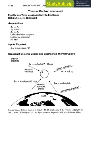
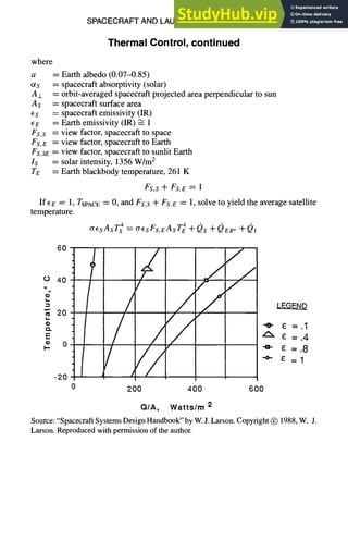
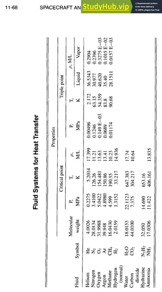
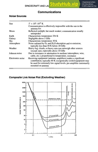
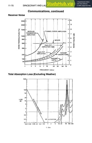
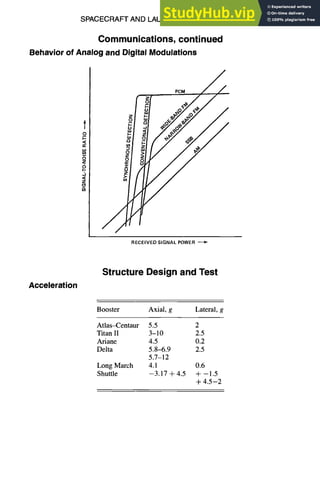
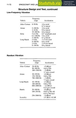
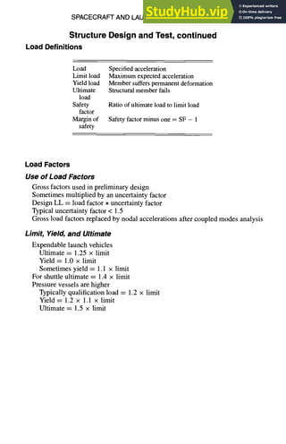
![11-74 SPACECRAFT
AND LAUNCHVEHICLE DESIGN
Structure Design and Test, continued
Spacecraft Structure Design/Verification
Launch
vehicle
constraints
Preliminary launch
loads from launch
vehicle user's manual
Launch vehicle
dynamic model
and forcing
function
Coupled launch
vehicle/spacecraft
dynamic analysis
t
Spacecraft dynamic
response
Loads
Accelerations
Compare preliminary
loads with update
loads and modify
structural design, if
necessary
Spacecraft ]
dynamic z
model
Spacecraft
structural
configuration
. [ Preliminary
. spacecraft
I structural design
I.
Structural analysis
Finite element model
Dynamic analysis
Stress analysis
Thermal distortion
Functional
requirements
of subsystems
Natural frequency
constraints
Thermal analysis
Fabricate spacecraft ]
structure
Temperature
distribution
I Environmentaltesting ]
I I
Ista'iotestingllsinetes'ingllAcoustintes'ing I
Source: Designof Geosynchronous Spacecraftby B. N. Agrawal. Copyright (~) 1986,
Prentice-Hall, Englewood Cliffs, NJ. Reprinted by permission of Prentice-Hall, Inc.](https://image.slidesharecdn.com/aiaaaerospacedesignengineersguide-230807164453-d76eba30/85/Aiaa-Aerospace-Design-Engineers-Guide-pdf-436-320.jpg)


This document provides an overview and introduction to the 5th edition of the AIAA Aerospace Design Engineers Guide. It discusses the guide's purpose of providing commonly used engineering reference data and general reference information for aerospace design disciplines. It also outlines some key systems engineering concepts for design engineers to consider, including understanding customer needs, developing a concept of operations, reviewing requirements for completeness, and using trade study methods to develop the product design.