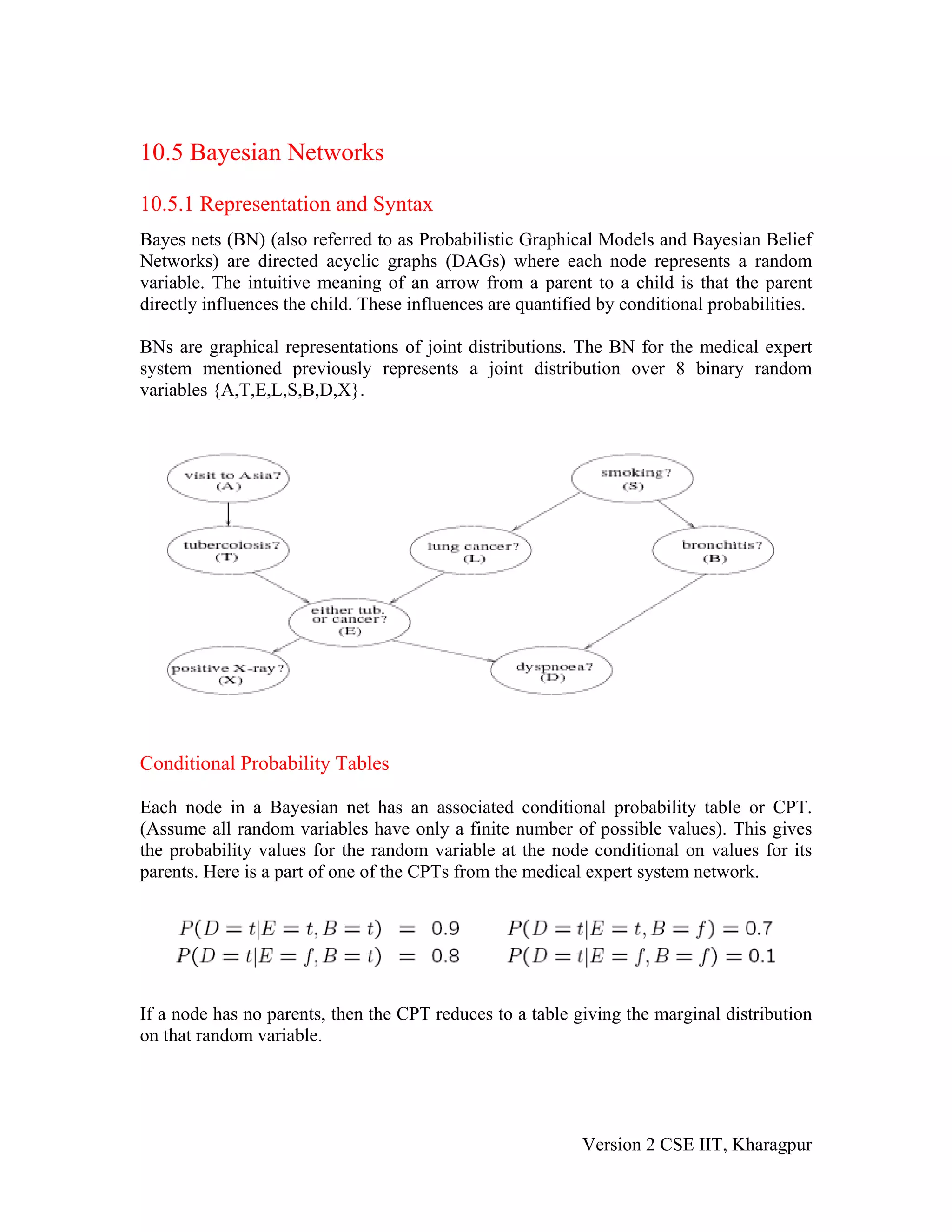
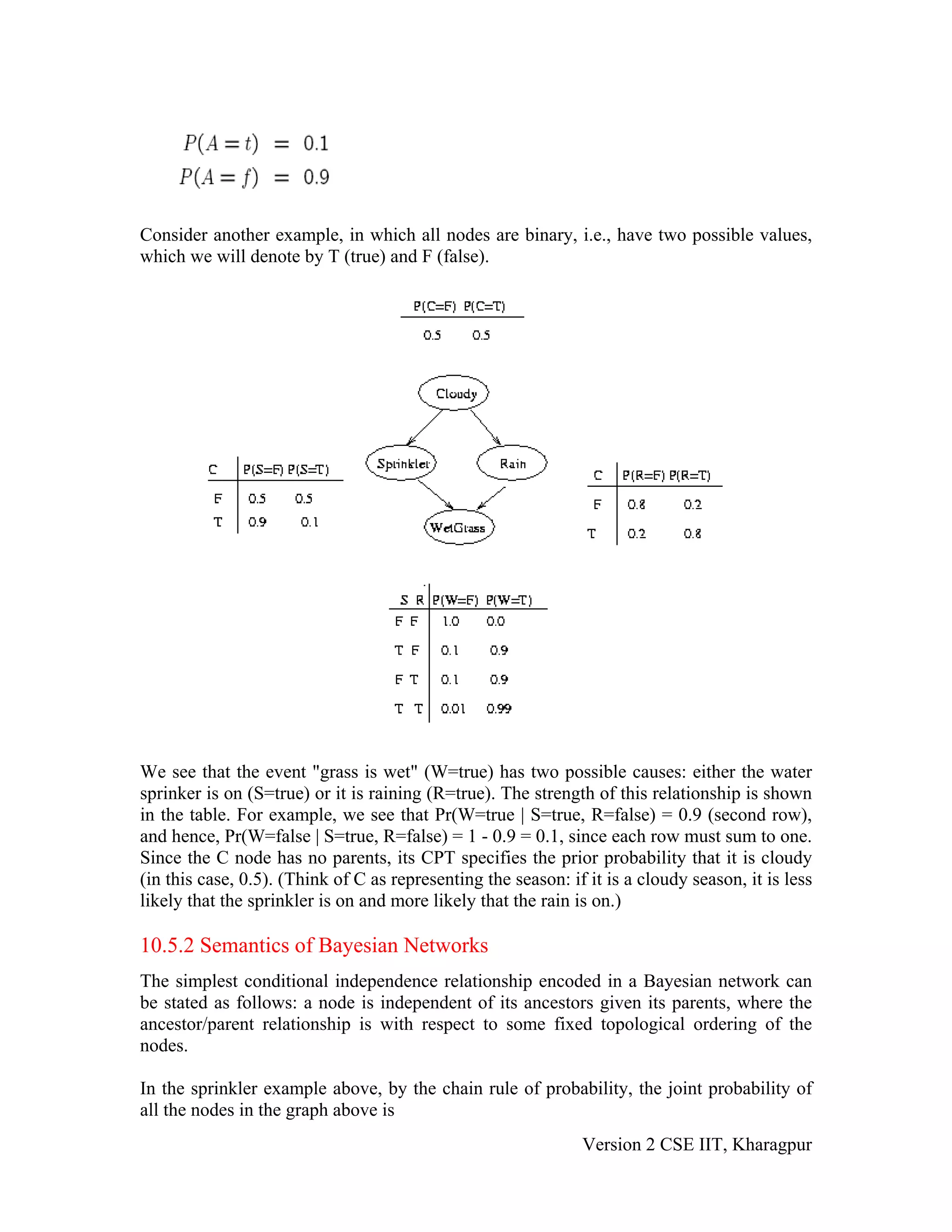
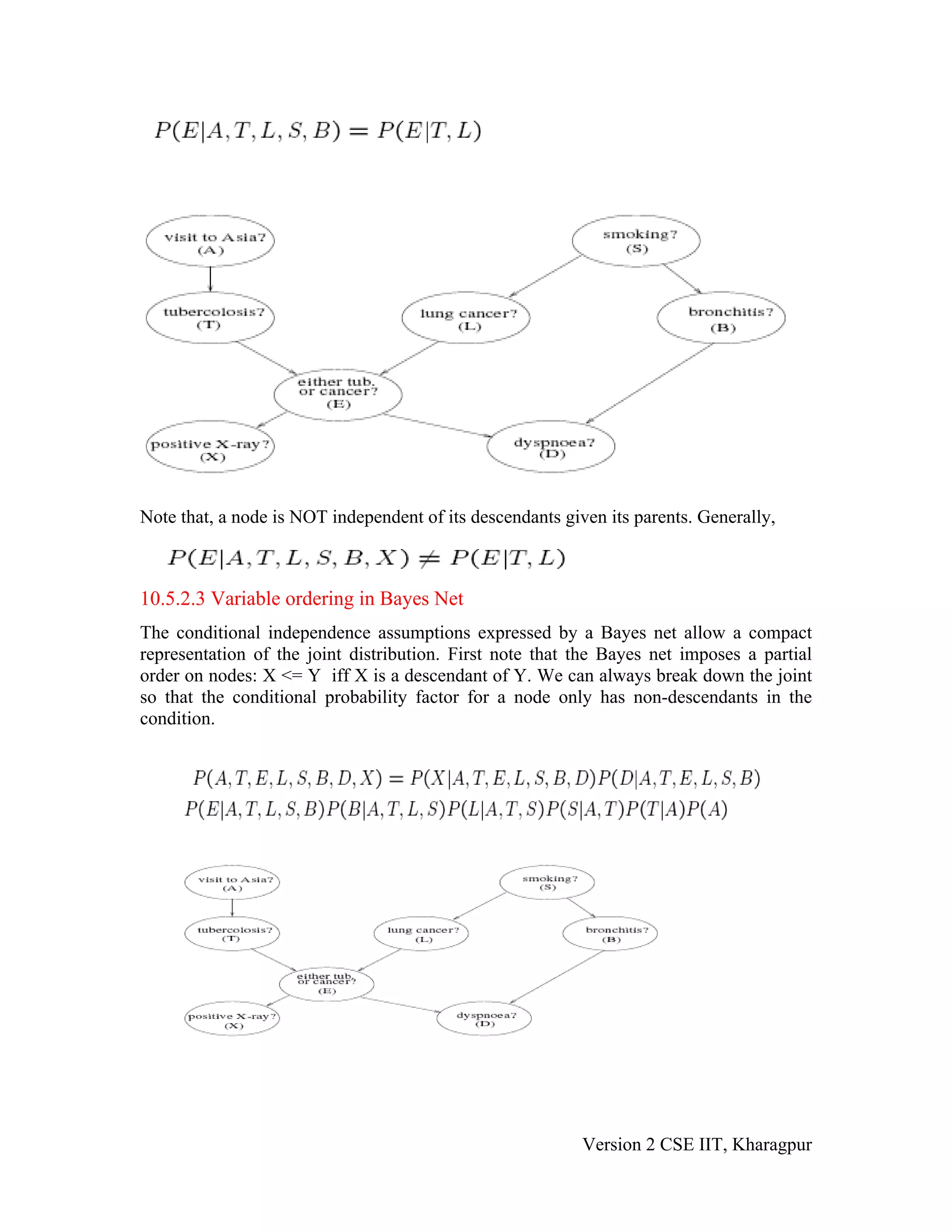
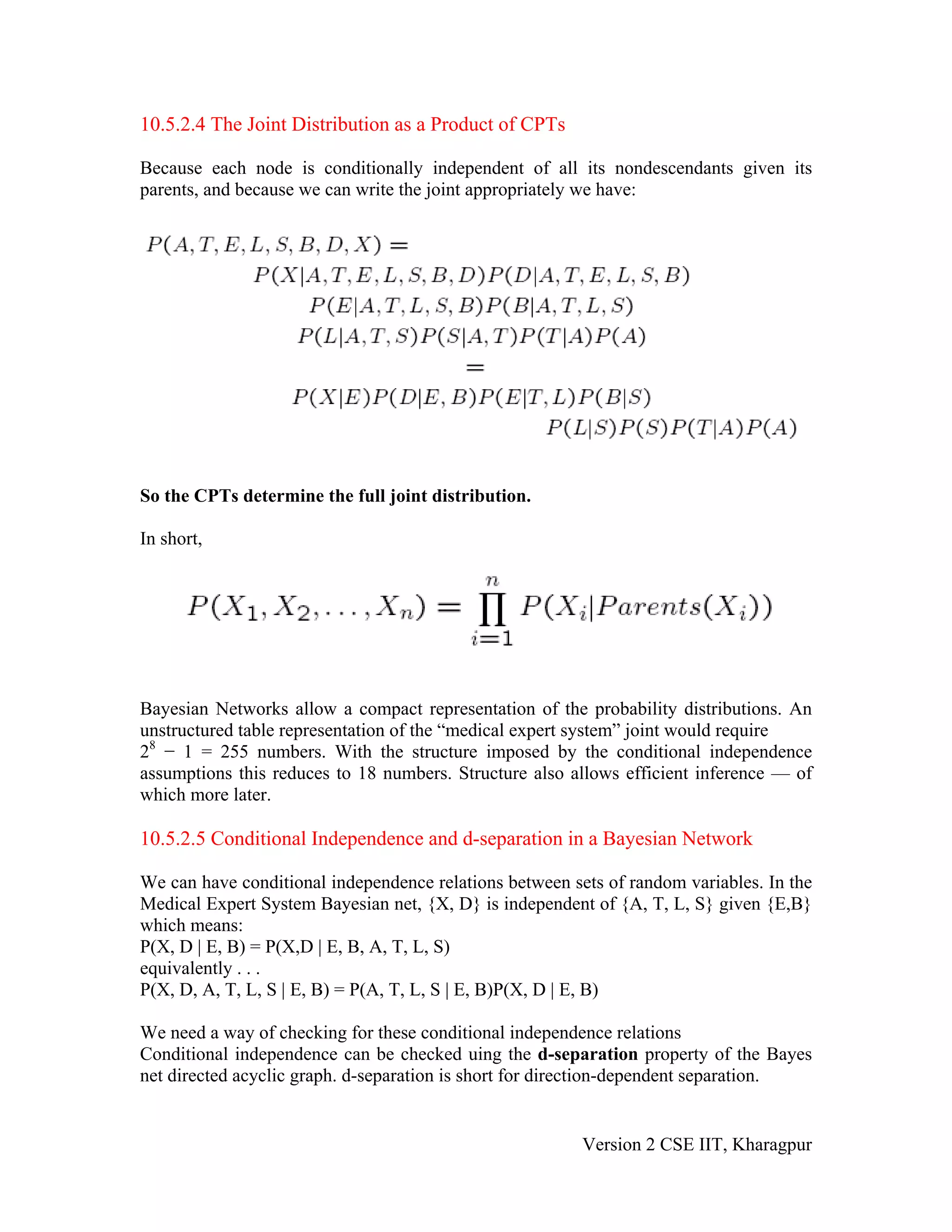
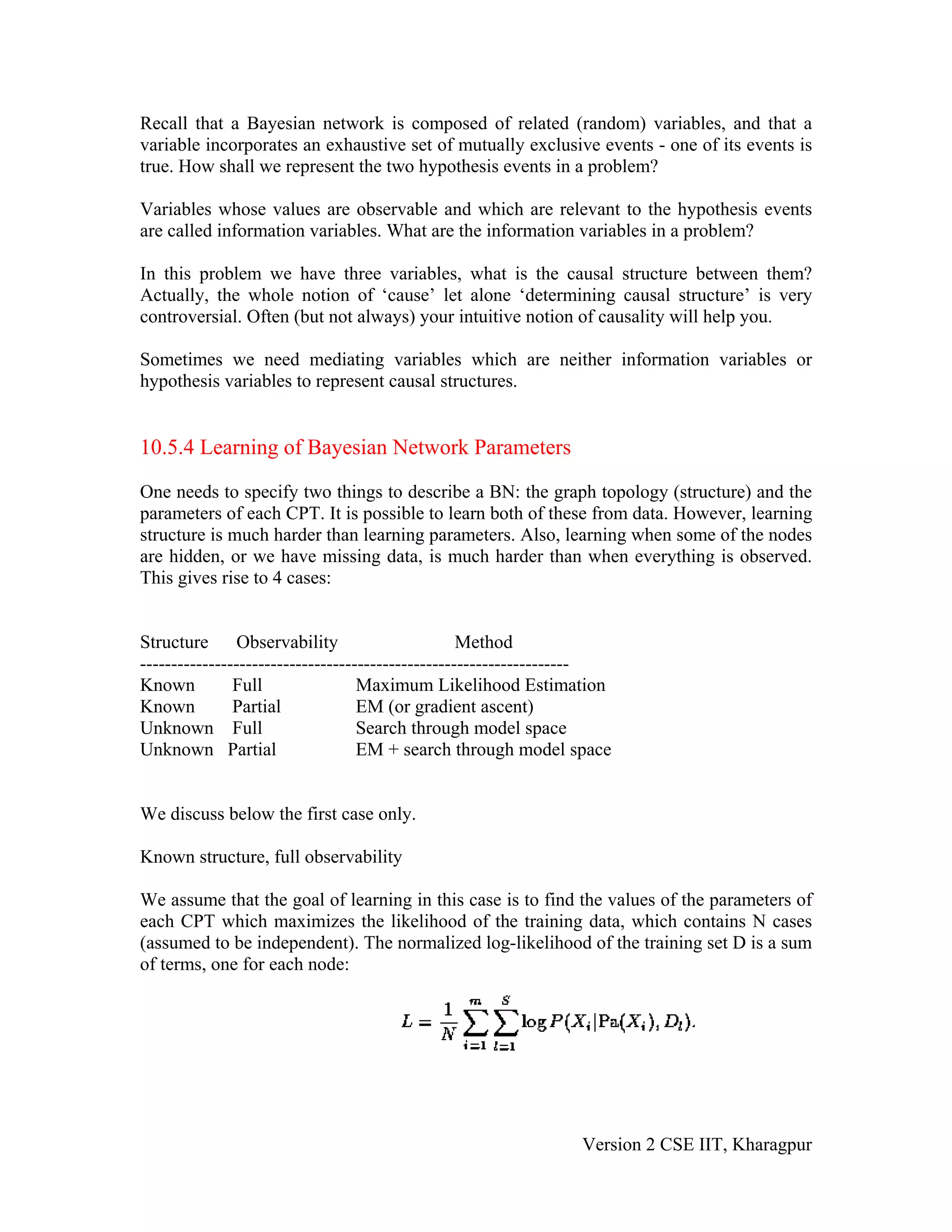
SlideShare a Scribd company logo
Module
                10
       Reasoning with
          Uncertainty -
Probabilistic reasoning

              Version 2 CSE IIT, Kharagpur
Lesson
         28
Bayes Networks
      Version 2 CSE IIT, Kharagpur
10.5 Bayesian Networks

10.5.1 Representation and Syntax
Bayes nets (BN) (also referred to as Probabilistic Graphical Models and Bayesian Belief
Networks) are directed acyclic graphs (DAGs) where each node represents a random
variable. The intuitive meaning of an arrow from a parent to a child is that the parent
directly influences the child. These influences are quantified by conditional probabilities.

BNs are graphical representations of joint distributions. The BN for the medical expert
system mentioned previously represents a joint distribution over 8 binary random
variables {A,T,E,L,S,B,D,X}.


Conditional Probability Tables

Each node in a Bayesian net has an associated conditional probability table or CPT.
(Assume all random variables have only a finite number of possible values). This gives
the probability values for the random variable at the node conditional on values for its
parents. Here is a part of one of the CPTs from the medical expert system network.


If a node has no parents, then the CPT reduces to a table giving the marginal distribution
on that random variable.


                                                            Version 2 CSE IIT, Kharagpur
Consider another example, in which all nodes are binary, i.e., have two possible values,
which we will denote by T (true) and F (false).


We see that the event "grass is wet" (W=true) has two possible causes: either the water
sprinker is on (S=true) or it is raining (R=true). The strength of this relationship is shown
in the table. For example, we see that Pr(W=true | S=true, R=false) = 0.9 (second row),
and hence, Pr(W=false | S=true, R=false) = 1 - 0.9 = 0.1, since each row must sum to one.
Since the C node has no parents, its CPT specifies the prior probability that it is cloudy
(in this case, 0.5). (Think of C as representing the season: if it is a cloudy season, it is less
likely that the sprinkler is on and more likely that the rain is on.)

10.5.2 Semantics of Bayesian Networks
The simplest conditional independence relationship encoded in a Bayesian network can
be stated as follows: a node is independent of its ancestors given its parents, where the
ancestor/parent relationship is with respect to some fixed topological ordering of the
nodes.

In the sprinkler example above, by the chain rule of probability, the joint probability of
all the nodes in the graph above is
                                                               Version 2 CSE IIT, Kharagpur
P(C, S, R, W) = P(C) * P(S|C) * P(R|C,S) * P(W|C,S,R)

By using conditional independence relationships, we can rewrite this as

P(C, S, R, W) = P(C) * P(S|C) * P(R|C) * P(W|S,R)

where we were allowed to simplify the third term because R is independent of S given its
parent C, and the last term because W is independent of C given its parents S and R. We
can see that the conditional independence relationships allow us to represent the joint
more compactly. Here the savings are minimal, but in general, if we had n binary nodes,
the full joint would require O(2^n) space to represent, but the factored form would
require O(n 2^k) space to represent, where k is the maximum fan-in of a node. And fewer
parameters makes learning easier.

The intuitive meaning of an arrow from a parent to a child is that the parent directly
influences the child. The direction of this influence is often taken to represent casual
influence. The conditional probabilities give the strength of causal influence. A 0 or 1 in
a CPT represents a deterministic influence.


10.5.2.1 Decomposing Joint Distributions

A joint distribution can always be broken down into a product of conditional probabilities
using repeated applications of the product rule.


We can order the variables however we like:


10.5.2.2 Conditional Independence in Bayes Net
A Bayes net represents the assumption that each node is conditionally independent of all
its non-descendants given its parents.

So for example,


                                                           Version 2 CSE IIT, Kharagpur
Note that, a node is NOT independent of its descendants given its parents. Generally,


10.5.2.3 Variable ordering in Bayes Net
The conditional independence assumptions expressed by a Bayes net allow a compact
representation of the joint distribution. First note that the Bayes net imposes a partial
order on nodes: X <= Y iff X is a descendant of Y. We can always break down the joint
so that the conditional probability factor for a node only has non-descendants in the
condition.


                                                           Version 2 CSE IIT, Kharagpur
10.5.2.4 The Joint Distribution as a Product of CPTs

Because each node is conditionally independent of all its nondescendants given its
parents, and because we can write the joint appropriately we have:


So the CPTs determine the full joint distribution.

In short,


Bayesian Networks allow a compact representation of the probability distributions. An
unstructured table representation of the “medical expert system” joint would require
28 − 1 = 255 numbers. With the structure imposed by the conditional independence
assumptions this reduces to 18 numbers. Structure also allows efficient inference — of
which more later.

10.5.2.5 Conditional Independence and d-separation in a Bayesian Network

We can have conditional independence relations between sets of random variables. In the
Medical Expert System Bayesian net, {X, D} is independent of {A, T, L, S} given {E,B}
which means:
P(X, D | E, B) = P(X,D | E, B, A, T, L, S)
equivalently . . .
P(X, D, A, T, L, S | E, B) = P(A, T, L, S | E, B)P(X, D | E, B)

We need a way of checking for these conditional independence relations
Conditional independence can be checked uing the d-separation property of the Bayes
net directed acyclic graph. d-separation is short for direction-dependent separation.


                                                         Version 2 CSE IIT, Kharagpur
If E d-separates X and Y then X and Y are conditionally independent given E.

E d-separates X and Y if every undirected path from a node in X to a node in Y is
blocked given E.

Defining d-separation:

A path is blocked given a set of nodes E if there is a node Z on the path for which one of
these three conditions holds:

1. Z is in E and Z has one arrow on the path coming in and one arrow going out.

2. Z is in E and Z has both path arrows leading out.

3. Neither Z nor any descendant of Z is in E, and both path arrows lead in to Z.

10.5.3 Building a Bayes Net: The Family Out? Example

We start with a natural language description of the situation to be modeled:

I want to know if my family is at home as I approach the house. Often my wife leaves on
a light when she goes out, but also sometimes if she is expecting a guest. When nobody is
home the dog is put in the back yard, but he is also put there when he has bowel trouble.
If the dog is in the back yard, I will hear her barking, but I may be confused by other dogs
barking.

Building the Bayes net involves the following steps.

We build Bayes nets to get probabilities concerning what we don’t know given what we
do know. What we don’t know is not observable. These are called hypothesis events – we
need to know what are the hypothesis events in a problem?


                                                            Version 2 CSE IIT, Kharagpur
Recall that a Bayesian network is composed of related (random) variables, and that a
variable incorporates an exhaustive set of mutually exclusive events - one of its events is
true. How shall we represent the two hypothesis events in a problem?

Variables whose values are observable and which are relevant to the hypothesis events
are called information variables. What are the information variables in a problem?

In this problem we have three variables, what is the causal structure between them?
Actually, the whole notion of ‘cause’ let alone ‘determining causal structure’ is very
controversial. Often (but not always) your intuitive notion of causality will help you.

Sometimes we need mediating variables which are neither information variables or
hypothesis variables to represent causal structures.


10.5.4 Learning of Bayesian Network Parameters

One needs to specify two things to describe a BN: the graph topology (structure) and the
parameters of each CPT. It is possible to learn both of these from data. However, learning
structure is much harder than learning parameters. Also, learning when some of the nodes
are hidden, or we have missing data, is much harder than when everything is observed.
This gives rise to 4 cases:


Structure Observability                            Method
---------------------------------------------------------------------
Known          Full                Maximum Likelihood Estimation
Known          Partial             EM (or gradient ascent)
Unknown Full                       Search through model space
Unknown Partial                    EM + search through model space


We discuss below the first case only.

Known structure, full observability

We assume that the goal of learning in this case is to find the values of the parameters of
each CPT which maximizes the likelihood of the training data, which contains N cases
(assumed to be independent). The normalized log-likelihood of the training set D is a sum
of terms, one for each node:


                                                                Version 2 CSE IIT, Kharagpur
We see that the log-likelihood scoring function decomposes according to the structure of
the graph, and hence we can maximize the contribution to the log-likelihood of each node
independently (assuming the parameters in each node are independent of the other
nodes). In cases where N is small compared to the number of parameters that require
fitting, we can use a numerical prior to regularize the problem. In this case, we call the
estimates Maximum A Posterori (MAP) estimates, as opposed to Maximum Likelihood
(ML) estimates.

Consider estimating the Conditional Probability Table for the W node. If we have a set of
training data, we can just count the number of times the grass is wet when it is raining
and the sprinler is on, N(W=1,S=1,R=1), the number of times the grass is wet when it is
raining and the sprinkler is off, N(W=1,S=0,R=1), etc. Given these counts (which are the
sufficient statistics), we can find the Maximum Likelihood Estimate of the CPT as
follows:


where the denominator is N(S=s,R=r) = N(W=0,S=s,R=r) + N(W=1,S=s,R=r). Thus
"learning" just amounts to counting (in the case of multinomial distributions). For
Gaussian nodes, we can compute the sample mean and variance, and use linear regression
to estimate the weight matrix. For other kinds of distributions, more complex procedures
are necessary.

As is well known from the HMM literature, ML estimates of CPTs are prone to sparse
data problems, which can be solved by using (mixtures of) Dirichlet priors (pseudo
counts). This results in a Maximum A Posteriori (MAP) estimate. For Gaussians, we can
use a Wishart prior, etc.


                                                           Version 2 CSE IIT, Kharagpur

More Related Content

What's hot

PRML Chapter 5
PRML Chapter 5PRML Chapter 5
PRML Chapter 5
Sunwoo Kim
 
PRML Chapter 1
PRML Chapter 1PRML Chapter 1
PRML Chapter 1
Sunwoo Kim
 
PRML Chapter 11
PRML Chapter 11PRML Chapter 11
PRML Chapter 11
Sunwoo Kim
 
Fuzzy logic
Fuzzy logicFuzzy logic
Fuzzy logic
Nateshwar Kamlesh
 
PRML Chapter 12
PRML Chapter 12PRML Chapter 12
PRML Chapter 12
Sunwoo Kim
 
PRML Chapter 10
PRML Chapter 10PRML Chapter 10
PRML Chapter 10
Sunwoo Kim
 
PRML Chapter 7
PRML Chapter 7PRML Chapter 7
PRML Chapter 7
Sunwoo Kim
 
PRML Chapter 6
PRML Chapter 6PRML Chapter 6
PRML Chapter 6
Sunwoo Kim
 
Fuzzy logic
Fuzzy logicFuzzy logic
Fuzzy logic
Mahmoud Hussein
 
PRML Chapter 8
PRML Chapter 8PRML Chapter 8
PRML Chapter 8
Sunwoo Kim
 
Fuzzy Membership Function
Fuzzy Membership Function Fuzzy Membership Function
PRML Chapter 2
PRML Chapter 2PRML Chapter 2
PRML Chapter 2
Sunwoo Kim
 
Fuzzy logic Notes AI CSE 8th Sem
Fuzzy logic Notes AI CSE 8th SemFuzzy logic Notes AI CSE 8th Sem
Fuzzy logic Notes AI CSE 8th Sem
DigiGurukul
 
Optimization using soft computing
Optimization using soft computingOptimization using soft computing
Optimization using soft computing
Purnima Pandit
 
Fuzzy Logic Ppt
Fuzzy Logic PptFuzzy Logic Ppt
Fuzzy Logic Pptrafi
 
Lec 5 uncertainty
Lec 5 uncertaintyLec 5 uncertainty
Lec 5 uncertainty
Eyob Sisay
 
Fuzzy Logic ppt
Fuzzy Logic pptFuzzy Logic ppt
Fuzzy Logic ppt
Ritu Bafna
 

What's hot (19)

PRML Chapter 5
PRML Chapter 5PRML Chapter 5
PRML Chapter 5
 
PRML Chapter 1
PRML Chapter 1PRML Chapter 1
PRML Chapter 1
 
PRML Chapter 11
PRML Chapter 11PRML Chapter 11
PRML Chapter 11
 
Fuzzy logic
Fuzzy logicFuzzy logic
Fuzzy logic
 
PRML Chapter 12
PRML Chapter 12PRML Chapter 12
PRML Chapter 12
 
PRML Chapter 10
PRML Chapter 10PRML Chapter 10
PRML Chapter 10
 
PRML Chapter 7
PRML Chapter 7PRML Chapter 7
PRML Chapter 7
 
PRML Chapter 6
PRML Chapter 6PRML Chapter 6
PRML Chapter 6
 
Fuzzy logic
Fuzzy logicFuzzy logic
Fuzzy logic
 
PRML Chapter 8
PRML Chapter 8PRML Chapter 8
PRML Chapter 8
 
Fuzzy Membership Function
Fuzzy Membership Function Fuzzy Membership Function
Fuzzy Membership Function
 
PRML Chapter 2
PRML Chapter 2PRML Chapter 2
PRML Chapter 2
 
Fuzzy logic Notes AI CSE 8th Sem
Fuzzy logic Notes AI CSE 8th SemFuzzy logic Notes AI CSE 8th Sem
Fuzzy logic Notes AI CSE 8th Sem
 
fuzzy logic
fuzzy logicfuzzy logic
fuzzy logic
 
Optimization using soft computing
Optimization using soft computingOptimization using soft computing
Optimization using soft computing
 
Fuzzy Logic Ppt
Fuzzy Logic PptFuzzy Logic Ppt
Fuzzy Logic Ppt
 
Lesson 32
Lesson 32Lesson 32
Lesson 32
 
Lec 5 uncertainty
Lec 5 uncertaintyLec 5 uncertainty
Lec 5 uncertainty
 
Fuzzy Logic ppt
Fuzzy Logic pptFuzzy Logic ppt
Fuzzy Logic ppt
 

Viewers also liked

Fuzzy logic - copy
Fuzzy logic - copyFuzzy logic - copy
Fuzzy logic - copy
Basil John
 
L 27(tb)(et) ((ee)nptel)
L 27(tb)(et) ((ee)nptel)L 27(tb)(et) ((ee)nptel)
L 27(tb)(et) ((ee)nptel)Pradeep Godara
 

Viewers also liked (8)

Fuzzy logic - copy
Fuzzy logic - copyFuzzy logic - copy
Fuzzy logic - copy
 
AI Lesson 31
AI Lesson 31AI Lesson 31
AI Lesson 31
 
AI Lesson 30
AI Lesson 30AI Lesson 30
AI Lesson 30
 
AI Lesson 27
AI Lesson 27AI Lesson 27
AI Lesson 27
 
AI Lesson 25
AI Lesson 25AI Lesson 25
AI Lesson 25
 
L 27(tb)(et) ((ee)nptel)
L 27(tb)(et) ((ee)nptel)L 27(tb)(et) ((ee)nptel)
L 27(tb)(et) ((ee)nptel)
 
AI Lesson 09
AI Lesson 09AI Lesson 09
AI Lesson 09
 
L15 fuzzy logic
L15  fuzzy logicL15  fuzzy logic
L15 fuzzy logic
 

Similar to AI Lesson 28

Reasoning Over Knowledge Base
Reasoning Over Knowledge BaseReasoning Over Knowledge Base
Reasoning Over Knowledge Base
Shubham Agarwal
 
Reasoning Over Knowledge Base
Reasoning Over Knowledge BaseReasoning Over Knowledge Base
Reasoning Over Knowledge Base
Shubham Agarwal
 
On the identifiability of phylogenetic networks under a pseudolikelihood model
On the identifiability of phylogenetic networks under a pseudolikelihood modelOn the identifiability of phylogenetic networks under a pseudolikelihood model
On the identifiability of phylogenetic networks under a pseudolikelihood model
Arrigo Coen
 
pcse.pdf
pcse.pdfpcse.pdf
pcse.pdf
LalaLebay
 
Quantum Deep Learning
Quantum Deep LearningQuantum Deep Learning
Quantum Deep Learning
Willy Marroquin (WillyDevNET)
 
A statistical criterion for reducing indeterminacy in linear causal modeling
A statistical criterion for reducing indeterminacy in linear causal modelingA statistical criterion for reducing indeterminacy in linear causal modeling
A statistical criterion for reducing indeterminacy in linear causal modeling
Gianluca Bontempi
 
A PROBABILISTIC ALGORITHM OF COMPUTING THE POLYNOMIAL GREATEST COMMON DIVISOR...
A PROBABILISTIC ALGORITHM OF COMPUTING THE POLYNOMIAL GREATEST COMMON DIVISOR...A PROBABILISTIC ALGORITHM OF COMPUTING THE POLYNOMIAL GREATEST COMMON DIVISOR...
A PROBABILISTIC ALGORITHM OF COMPUTING THE POLYNOMIAL GREATEST COMMON DIVISOR...
ijscmcj
 
712201907
712201907712201907
712201907
IJRAT
 
Bayesian Co clustering
Bayesian Co clusteringBayesian Co clustering
Bayesian Co clusteringlau
 
So sánh cấu trúc protein_Protein structure comparison
So sánh cấu trúc protein_Protein structure comparisonSo sánh cấu trúc protein_Protein structure comparison
So sánh cấu trúc protein_Protein structure comparison
bomxuan868
 
Bachelor's Thesis
Bachelor's ThesisBachelor's Thesis
Bachelor's Thesis
Bastiaan Frerix
 
A tutorial in Connectome Analysis (1) - Marcus Kaiser
A tutorial in Connectome Analysis (1) - Marcus KaiserA tutorial in Connectome Analysis (1) - Marcus Kaiser
A tutorial in Connectome Analysis (1) - Marcus Kaiser
Lake Como School of Advanced Studies
 
Improving Tree augmented Naive Bayes for class probability estimation
Improving Tree augmented Naive Bayes for class probability estimationImproving Tree augmented Naive Bayes for class probability estimation
Improving Tree augmented Naive Bayes for class probability estimation
Beat Winehouse
 
Redundancy elimination of_big_sensor_data_using_bayesian_networks (1)
Redundancy elimination of_big_sensor_data_using_bayesian_networks (1)Redundancy elimination of_big_sensor_data_using_bayesian_networks (1)
Redundancy elimination of_big_sensor_data_using_bayesian_networks (1)
Crislanio Macedo
 

Similar to AI Lesson 28 (20)

Reasoning Over Knowledge Base
Reasoning Over Knowledge BaseReasoning Over Knowledge Base
Reasoning Over Knowledge Base
 
Reasoning Over Knowledge Base
Reasoning Over Knowledge BaseReasoning Over Knowledge Base
Reasoning Over Knowledge Base
 
On the identifiability of phylogenetic networks under a pseudolikelihood model
On the identifiability of phylogenetic networks under a pseudolikelihood modelOn the identifiability of phylogenetic networks under a pseudolikelihood model
On the identifiability of phylogenetic networks under a pseudolikelihood model
 
Lesson 26
Lesson 26Lesson 26
Lesson 26
 
AI Lesson 26
AI Lesson 26AI Lesson 26
AI Lesson 26
 
AI Lesson 29
AI Lesson 29AI Lesson 29
AI Lesson 29
 
pcse.pdf
pcse.pdfpcse.pdf
pcse.pdf
 
Quantum Deep Learning
Quantum Deep LearningQuantum Deep Learning
Quantum Deep Learning
 
A statistical criterion for reducing indeterminacy in linear causal modeling
A statistical criterion for reducing indeterminacy in linear causal modelingA statistical criterion for reducing indeterminacy in linear causal modeling
A statistical criterion for reducing indeterminacy in linear causal modeling
 
A PROBABILISTIC ALGORITHM OF COMPUTING THE POLYNOMIAL GREATEST COMMON DIVISOR...
A PROBABILISTIC ALGORITHM OF COMPUTING THE POLYNOMIAL GREATEST COMMON DIVISOR...A PROBABILISTIC ALGORITHM OF COMPUTING THE POLYNOMIAL GREATEST COMMON DIVISOR...
A PROBABILISTIC ALGORITHM OF COMPUTING THE POLYNOMIAL GREATEST COMMON DIVISOR...
 
712201907
712201907712201907
712201907
 
Bayesian Co clustering
Bayesian Co clusteringBayesian Co clustering
Bayesian Co clustering
 
So sánh cấu trúc protein_Protein structure comparison
So sánh cấu trúc protein_Protein structure comparisonSo sánh cấu trúc protein_Protein structure comparison
So sánh cấu trúc protein_Protein structure comparison
 
Bachelor's Thesis
Bachelor's ThesisBachelor's Thesis
Bachelor's Thesis
 
A tutorial in Connectome Analysis (1) - Marcus Kaiser
A tutorial in Connectome Analysis (1) - Marcus KaiserA tutorial in Connectome Analysis (1) - Marcus Kaiser
A tutorial in Connectome Analysis (1) - Marcus Kaiser
 
Fuzzy
FuzzyFuzzy
Fuzzy
 
Ch 6 final
Ch 6 finalCh 6 final
Ch 6 final
 
Improving Tree augmented Naive Bayes for class probability estimation
Improving Tree augmented Naive Bayes for class probability estimationImproving Tree augmented Naive Bayes for class probability estimation
Improving Tree augmented Naive Bayes for class probability estimation
 
Redundancy elimination of_big_sensor_data_using_bayesian_networks (1)
Redundancy elimination of_big_sensor_data_using_bayesian_networks (1)Redundancy elimination of_big_sensor_data_using_bayesian_networks (1)
Redundancy elimination of_big_sensor_data_using_bayesian_networks (1)
 
graph_embeddings
graph_embeddingsgraph_embeddings
graph_embeddings
 

More from Assistant Professor (20)

AI Lesson 41
AI Lesson 41AI Lesson 41
AI Lesson 41
 
AI Lesson 40
AI Lesson 40AI Lesson 40
AI Lesson 40
 
AI Lesson 39
AI Lesson 39AI Lesson 39
AI Lesson 39
 
AI Lesson 38
AI Lesson 38AI Lesson 38
AI Lesson 38
 
AI Lesson 37
AI Lesson 37AI Lesson 37
AI Lesson 37
 
AI Lesson 36
AI Lesson 36AI Lesson 36
AI Lesson 36
 
AI Lesson 35
AI Lesson 35AI Lesson 35
AI Lesson 35
 
AI Lesson 33
AI Lesson 33AI Lesson 33
AI Lesson 33
 
AI Lesson 32
AI Lesson 32AI Lesson 32
AI Lesson 32
 
AI Lesson 24
AI Lesson 24AI Lesson 24
AI Lesson 24
 
AI Lesson 23
AI Lesson 23AI Lesson 23
AI Lesson 23
 
AI Lesson 22
AI Lesson 22AI Lesson 22
AI Lesson 22
 
AI Lesson 21
AI Lesson 21AI Lesson 21
AI Lesson 21
 
Lesson 20
Lesson 20Lesson 20
Lesson 20
 
AI Lesson 19
AI Lesson 19AI Lesson 19
AI Lesson 19
 
AI Lesson 18
AI Lesson 18AI Lesson 18
AI Lesson 18
 
AI Lesson 17
AI Lesson 17AI Lesson 17
AI Lesson 17
 
AI Lesson 16
AI Lesson 16AI Lesson 16
AI Lesson 16
 
AI Lesson 15
AI Lesson 15AI Lesson 15
AI Lesson 15
 
AI Lesson 14
AI Lesson 14AI Lesson 14
AI Lesson 14
 

Recently uploaded

A Strategic Approach: GenAI in Education
A Strategic Approach: GenAI in EducationA Strategic Approach: GenAI in Education
A Strategic Approach: GenAI in Education
Peter Windle
 
The French Revolution Class 9 Study Material pdf free download
The French Revolution Class 9 Study Material pdf free downloadThe French Revolution Class 9 Study Material pdf free download
The French Revolution Class 9 Study Material pdf free download
Vivekanand Anglo Vedic Academy
 
Overview on Edible Vaccine: Pros & Cons with Mechanism
Overview on Edible Vaccine: Pros & Cons with MechanismOverview on Edible Vaccine: Pros & Cons with Mechanism
Overview on Edible Vaccine: Pros & Cons with Mechanism
DeeptiGupta154
 
1.4 modern child centered education - mahatma gandhi-2.pptx
1.4 modern child centered education - mahatma gandhi-2.pptx1.4 modern child centered education - mahatma gandhi-2.pptx
1.4 modern child centered education - mahatma gandhi-2.pptx
JosvitaDsouza2
 
Guidance_and_Counselling.pdf B.Ed. 4th Semester
Guidance_and_Counselling.pdf B.Ed. 4th SemesterGuidance_and_Counselling.pdf B.Ed. 4th Semester
Guidance_and_Counselling.pdf B.Ed. 4th Semester
Atul Kumar Singh
 
Unit 8 - Information and Communication Technology (Paper I).pdf
Unit 8 - Information and Communication Technology (Paper I).pdfUnit 8 - Information and Communication Technology (Paper I).pdf
Unit 8 - Information and Communication Technology (Paper I).pdf
Thiyagu K
 
BÀI TẬP BỔ TRỢ TIẾNG ANH GLOBAL SUCCESS LỚP 3 - CẢ NĂM (CÓ FILE NGHE VÀ ĐÁP Á...
BÀI TẬP BỔ TRỢ TIẾNG ANH GLOBAL SUCCESS LỚP 3 - CẢ NĂM (CÓ FILE NGHE VÀ ĐÁP Á...BÀI TẬP BỔ TRỢ TIẾNG ANH GLOBAL SUCCESS LỚP 3 - CẢ NĂM (CÓ FILE NGHE VÀ ĐÁP Á...
BÀI TẬP BỔ TRỢ TIẾNG ANH GLOBAL SUCCESS LỚP 3 - CẢ NĂM (CÓ FILE NGHE VÀ ĐÁP Á...
Nguyen Thanh Tu Collection
 
2024.06.01 Introducing a competency framework for languag learning materials ...
2024.06.01 Introducing a competency framework for languag learning materials ...2024.06.01 Introducing a competency framework for languag learning materials ...
2024.06.01 Introducing a competency framework for languag learning materials ...
Sandy Millin
 
The approach at University of Liverpool.pptx
The approach at University of Liverpool.pptxThe approach at University of Liverpool.pptx
The approach at University of Liverpool.pptx
Jisc
 
TESDA TM1 REVIEWER FOR NATIONAL ASSESSMENT WRITTEN AND ORAL QUESTIONS WITH A...
TESDA TM1 REVIEWER  FOR NATIONAL ASSESSMENT WRITTEN AND ORAL QUESTIONS WITH A...TESDA TM1 REVIEWER  FOR NATIONAL ASSESSMENT WRITTEN AND ORAL QUESTIONS WITH A...
TESDA TM1 REVIEWER FOR NATIONAL ASSESSMENT WRITTEN AND ORAL QUESTIONS WITH A...
EugeneSaldivar
 
aaaaaaaaaaaaaaaaaaaaaaaaaaaaaaaaaaaaaaaaa
aaaaaaaaaaaaaaaaaaaaaaaaaaaaaaaaaaaaaaaaaaaaaaaaaaaaaaaaaaaaaaaaaaaaaaaaaaaaaaaaaa
aaaaaaaaaaaaaaaaaaaaaaaaaaaaaaaaaaaaaaaaa
siemaillard
 
The Challenger.pdf DNHS Official Publication
The Challenger.pdf DNHS Official PublicationThe Challenger.pdf DNHS Official Publication
The Challenger.pdf DNHS Official Publication
Delapenabediema
 
Chapter -12, Antibiotics (One Page Notes).pdf
Chapter -12, Antibiotics (One Page Notes).pdfChapter -12, Antibiotics (One Page Notes).pdf
Chapter -12, Antibiotics (One Page Notes).pdf
Kartik Tiwari
 
June 3, 2024 Anti-Semitism Letter Sent to MIT President Kornbluth and MIT Cor...
June 3, 2024 Anti-Semitism Letter Sent to MIT President Kornbluth and MIT Cor...June 3, 2024 Anti-Semitism Letter Sent to MIT President Kornbluth and MIT Cor...
June 3, 2024 Anti-Semitism Letter Sent to MIT President Kornbluth and MIT Cor...
Levi Shapiro
 
Honest Reviews of Tim Han LMA Course Program.pptx
Honest Reviews of Tim Han LMA Course Program.pptxHonest Reviews of Tim Han LMA Course Program.pptx
Honest Reviews of Tim Han LMA Course Program.pptx
timhan337
 
How libraries can support authors with open access requirements for UKRI fund...
How libraries can support authors with open access requirements for UKRI fund...How libraries can support authors with open access requirements for UKRI fund...
How libraries can support authors with open access requirements for UKRI fund...
Jisc
 
Introduction to AI for Nonprofits with Tapp Network
Introduction to AI for Nonprofits with Tapp NetworkIntroduction to AI for Nonprofits with Tapp Network
Introduction to AI for Nonprofits with Tapp Network
TechSoup
 
Language Across the Curriculm LAC B.Ed.
Language Across the  Curriculm LAC B.Ed.Language Across the  Curriculm LAC B.Ed.
Language Across the Curriculm LAC B.Ed.
Atul Kumar Singh
 
How to Make a Field invisible in Odoo 17
How to Make a Field invisible in Odoo 17How to Make a Field invisible in Odoo 17
How to Make a Field invisible in Odoo 17
Celine George
 
Model Attribute Check Company Auto Property
Model Attribute  Check Company Auto PropertyModel Attribute  Check Company Auto Property
Model Attribute Check Company Auto Property
Celine George
 

Recently uploaded (20)

A Strategic Approach: GenAI in Education
A Strategic Approach: GenAI in EducationA Strategic Approach: GenAI in Education
A Strategic Approach: GenAI in Education
 
The French Revolution Class 9 Study Material pdf free download
The French Revolution Class 9 Study Material pdf free downloadThe French Revolution Class 9 Study Material pdf free download
The French Revolution Class 9 Study Material pdf free download
 
Overview on Edible Vaccine: Pros & Cons with Mechanism
Overview on Edible Vaccine: Pros & Cons with MechanismOverview on Edible Vaccine: Pros & Cons with Mechanism
Overview on Edible Vaccine: Pros & Cons with Mechanism
 
1.4 modern child centered education - mahatma gandhi-2.pptx
1.4 modern child centered education - mahatma gandhi-2.pptx1.4 modern child centered education - mahatma gandhi-2.pptx
1.4 modern child centered education - mahatma gandhi-2.pptx
 
Guidance_and_Counselling.pdf B.Ed. 4th Semester
Guidance_and_Counselling.pdf B.Ed. 4th SemesterGuidance_and_Counselling.pdf B.Ed. 4th Semester
Guidance_and_Counselling.pdf B.Ed. 4th Semester
 
Unit 8 - Information and Communication Technology (Paper I).pdf
Unit 8 - Information and Communication Technology (Paper I).pdfUnit 8 - Information and Communication Technology (Paper I).pdf
Unit 8 - Information and Communication Technology (Paper I).pdf
 
BÀI TẬP BỔ TRỢ TIẾNG ANH GLOBAL SUCCESS LỚP 3 - CẢ NĂM (CÓ FILE NGHE VÀ ĐÁP Á...
BÀI TẬP BỔ TRỢ TIẾNG ANH GLOBAL SUCCESS LỚP 3 - CẢ NĂM (CÓ FILE NGHE VÀ ĐÁP Á...BÀI TẬP BỔ TRỢ TIẾNG ANH GLOBAL SUCCESS LỚP 3 - CẢ NĂM (CÓ FILE NGHE VÀ ĐÁP Á...
BÀI TẬP BỔ TRỢ TIẾNG ANH GLOBAL SUCCESS LỚP 3 - CẢ NĂM (CÓ FILE NGHE VÀ ĐÁP Á...
 
2024.06.01 Introducing a competency framework for languag learning materials ...
2024.06.01 Introducing a competency framework for languag learning materials ...2024.06.01 Introducing a competency framework for languag learning materials ...
2024.06.01 Introducing a competency framework for languag learning materials ...
 
The approach at University of Liverpool.pptx
The approach at University of Liverpool.pptxThe approach at University of Liverpool.pptx
The approach at University of Liverpool.pptx
 
TESDA TM1 REVIEWER FOR NATIONAL ASSESSMENT WRITTEN AND ORAL QUESTIONS WITH A...
TESDA TM1 REVIEWER  FOR NATIONAL ASSESSMENT WRITTEN AND ORAL QUESTIONS WITH A...TESDA TM1 REVIEWER  FOR NATIONAL ASSESSMENT WRITTEN AND ORAL QUESTIONS WITH A...
TESDA TM1 REVIEWER FOR NATIONAL ASSESSMENT WRITTEN AND ORAL QUESTIONS WITH A...
 
aaaaaaaaaaaaaaaaaaaaaaaaaaaaaaaaaaaaaaaaa
aaaaaaaaaaaaaaaaaaaaaaaaaaaaaaaaaaaaaaaaaaaaaaaaaaaaaaaaaaaaaaaaaaaaaaaaaaaaaaaaaa
aaaaaaaaaaaaaaaaaaaaaaaaaaaaaaaaaaaaaaaaa
 
The Challenger.pdf DNHS Official Publication
The Challenger.pdf DNHS Official PublicationThe Challenger.pdf DNHS Official Publication
The Challenger.pdf DNHS Official Publication
 
Chapter -12, Antibiotics (One Page Notes).pdf
Chapter -12, Antibiotics (One Page Notes).pdfChapter -12, Antibiotics (One Page Notes).pdf
Chapter -12, Antibiotics (One Page Notes).pdf
 
June 3, 2024 Anti-Semitism Letter Sent to MIT President Kornbluth and MIT Cor...
June 3, 2024 Anti-Semitism Letter Sent to MIT President Kornbluth and MIT Cor...June 3, 2024 Anti-Semitism Letter Sent to MIT President Kornbluth and MIT Cor...
June 3, 2024 Anti-Semitism Letter Sent to MIT President Kornbluth and MIT Cor...
 
Honest Reviews of Tim Han LMA Course Program.pptx
Honest Reviews of Tim Han LMA Course Program.pptxHonest Reviews of Tim Han LMA Course Program.pptx
Honest Reviews of Tim Han LMA Course Program.pptx
 
How libraries can support authors with open access requirements for UKRI fund...
How libraries can support authors with open access requirements for UKRI fund...How libraries can support authors with open access requirements for UKRI fund...
How libraries can support authors with open access requirements for UKRI fund...
 
Introduction to AI for Nonprofits with Tapp Network
Introduction to AI for Nonprofits with Tapp NetworkIntroduction to AI for Nonprofits with Tapp Network
Introduction to AI for Nonprofits with Tapp Network
 
Language Across the Curriculm LAC B.Ed.
Language Across the  Curriculm LAC B.Ed.Language Across the  Curriculm LAC B.Ed.
Language Across the Curriculm LAC B.Ed.
 
How to Make a Field invisible in Odoo 17
How to Make a Field invisible in Odoo 17How to Make a Field invisible in Odoo 17
How to Make a Field invisible in Odoo 17
 
Model Attribute Check Company Auto Property
Model Attribute  Check Company Auto PropertyModel Attribute  Check Company Auto Property
Model Attribute Check Company Auto Property
 

AI Lesson 28

  • 1. Module 10 Reasoning with Uncertainty - Probabilistic reasoning Version 2 CSE IIT, Kharagpur
  • 2. Lesson 28 Bayes Networks Version 2 CSE IIT, Kharagpur
  • 3. 10.5 Bayesian Networks 10.5.1 Representation and Syntax Bayes nets (BN) (also referred to as Probabilistic Graphical Models and Bayesian Belief Networks) are directed acyclic graphs (DAGs) where each node represents a random variable. The intuitive meaning of an arrow from a parent to a child is that the parent directly influences the child. These influences are quantified by conditional probabilities. BNs are graphical representations of joint distributions. The BN for the medical expert system mentioned previously represents a joint distribution over 8 binary random variables {A,T,E,L,S,B,D,X}. Conditional Probability Tables Each node in a Bayesian net has an associated conditional probability table or CPT. (Assume all random variables have only a finite number of possible values). This gives the probability values for the random variable at the node conditional on values for its parents. Here is a part of one of the CPTs from the medical expert system network. If a node has no parents, then the CPT reduces to a table giving the marginal distribution on that random variable. Version 2 CSE IIT, Kharagpur
  • 4. Consider another example, in which all nodes are binary, i.e., have two possible values, which we will denote by T (true) and F (false). We see that the event "grass is wet" (W=true) has two possible causes: either the water sprinker is on (S=true) or it is raining (R=true). The strength of this relationship is shown in the table. For example, we see that Pr(W=true | S=true, R=false) = 0.9 (second row), and hence, Pr(W=false | S=true, R=false) = 1 - 0.9 = 0.1, since each row must sum to one. Since the C node has no parents, its CPT specifies the prior probability that it is cloudy (in this case, 0.5). (Think of C as representing the season: if it is a cloudy season, it is less likely that the sprinkler is on and more likely that the rain is on.) 10.5.2 Semantics of Bayesian Networks The simplest conditional independence relationship encoded in a Bayesian network can be stated as follows: a node is independent of its ancestors given its parents, where the ancestor/parent relationship is with respect to some fixed topological ordering of the nodes. In the sprinkler example above, by the chain rule of probability, the joint probability of all the nodes in the graph above is Version 2 CSE IIT, Kharagpur
  • 5. P(C, S, R, W) = P(C) * P(S|C) * P(R|C,S) * P(W|C,S,R) By using conditional independence relationships, we can rewrite this as P(C, S, R, W) = P(C) * P(S|C) * P(R|C) * P(W|S,R) where we were allowed to simplify the third term because R is independent of S given its parent C, and the last term because W is independent of C given its parents S and R. We can see that the conditional independence relationships allow us to represent the joint more compactly. Here the savings are minimal, but in general, if we had n binary nodes, the full joint would require O(2^n) space to represent, but the factored form would require O(n 2^k) space to represent, where k is the maximum fan-in of a node. And fewer parameters makes learning easier. The intuitive meaning of an arrow from a parent to a child is that the parent directly influences the child. The direction of this influence is often taken to represent casual influence. The conditional probabilities give the strength of causal influence. A 0 or 1 in a CPT represents a deterministic influence. 10.5.2.1 Decomposing Joint Distributions A joint distribution can always be broken down into a product of conditional probabilities using repeated applications of the product rule. We can order the variables however we like: 10.5.2.2 Conditional Independence in Bayes Net A Bayes net represents the assumption that each node is conditionally independent of all its non-descendants given its parents. So for example, Version 2 CSE IIT, Kharagpur
  • 6. Note that, a node is NOT independent of its descendants given its parents. Generally, 10.5.2.3 Variable ordering in Bayes Net The conditional independence assumptions expressed by a Bayes net allow a compact representation of the joint distribution. First note that the Bayes net imposes a partial order on nodes: X <= Y iff X is a descendant of Y. We can always break down the joint so that the conditional probability factor for a node only has non-descendants in the condition. Version 2 CSE IIT, Kharagpur
  • 7. 10.5.2.4 The Joint Distribution as a Product of CPTs Because each node is conditionally independent of all its nondescendants given its parents, and because we can write the joint appropriately we have: So the CPTs determine the full joint distribution. In short, Bayesian Networks allow a compact representation of the probability distributions. An unstructured table representation of the “medical expert system” joint would require 28 − 1 = 255 numbers. With the structure imposed by the conditional independence assumptions this reduces to 18 numbers. Structure also allows efficient inference — of which more later. 10.5.2.5 Conditional Independence and d-separation in a Bayesian Network We can have conditional independence relations between sets of random variables. In the Medical Expert System Bayesian net, {X, D} is independent of {A, T, L, S} given {E,B} which means: P(X, D | E, B) = P(X,D | E, B, A, T, L, S) equivalently . . . P(X, D, A, T, L, S | E, B) = P(A, T, L, S | E, B)P(X, D | E, B) We need a way of checking for these conditional independence relations Conditional independence can be checked uing the d-separation property of the Bayes net directed acyclic graph. d-separation is short for direction-dependent separation. Version 2 CSE IIT, Kharagpur
  • 8. If E d-separates X and Y then X and Y are conditionally independent given E. E d-separates X and Y if every undirected path from a node in X to a node in Y is blocked given E. Defining d-separation: A path is blocked given a set of nodes E if there is a node Z on the path for which one of these three conditions holds: 1. Z is in E and Z has one arrow on the path coming in and one arrow going out. 2. Z is in E and Z has both path arrows leading out. 3. Neither Z nor any descendant of Z is in E, and both path arrows lead in to Z. 10.5.3 Building a Bayes Net: The Family Out? Example We start with a natural language description of the situation to be modeled: I want to know if my family is at home as I approach the house. Often my wife leaves on a light when she goes out, but also sometimes if she is expecting a guest. When nobody is home the dog is put in the back yard, but he is also put there when he has bowel trouble. If the dog is in the back yard, I will hear her barking, but I may be confused by other dogs barking. Building the Bayes net involves the following steps. We build Bayes nets to get probabilities concerning what we don’t know given what we do know. What we don’t know is not observable. These are called hypothesis events – we need to know what are the hypothesis events in a problem? Version 2 CSE IIT, Kharagpur
  • 9. Recall that a Bayesian network is composed of related (random) variables, and that a variable incorporates an exhaustive set of mutually exclusive events - one of its events is true. How shall we represent the two hypothesis events in a problem? Variables whose values are observable and which are relevant to the hypothesis events are called information variables. What are the information variables in a problem? In this problem we have three variables, what is the causal structure between them? Actually, the whole notion of ‘cause’ let alone ‘determining causal structure’ is very controversial. Often (but not always) your intuitive notion of causality will help you. Sometimes we need mediating variables which are neither information variables or hypothesis variables to represent causal structures. 10.5.4 Learning of Bayesian Network Parameters One needs to specify two things to describe a BN: the graph topology (structure) and the parameters of each CPT. It is possible to learn both of these from data. However, learning structure is much harder than learning parameters. Also, learning when some of the nodes are hidden, or we have missing data, is much harder than when everything is observed. This gives rise to 4 cases: Structure Observability Method --------------------------------------------------------------------- Known Full Maximum Likelihood Estimation Known Partial EM (or gradient ascent) Unknown Full Search through model space Unknown Partial EM + search through model space We discuss below the first case only. Known structure, full observability We assume that the goal of learning in this case is to find the values of the parameters of each CPT which maximizes the likelihood of the training data, which contains N cases (assumed to be independent). The normalized log-likelihood of the training set D is a sum of terms, one for each node: Version 2 CSE IIT, Kharagpur
  • 10. We see that the log-likelihood scoring function decomposes according to the structure of the graph, and hence we can maximize the contribution to the log-likelihood of each node independently (assuming the parameters in each node are independent of the other nodes). In cases where N is small compared to the number of parameters that require fitting, we can use a numerical prior to regularize the problem. In this case, we call the estimates Maximum A Posterori (MAP) estimates, as opposed to Maximum Likelihood (ML) estimates. Consider estimating the Conditional Probability Table for the W node. If we have a set of training data, we can just count the number of times the grass is wet when it is raining and the sprinler is on, N(W=1,S=1,R=1), the number of times the grass is wet when it is raining and the sprinkler is off, N(W=1,S=0,R=1), etc. Given these counts (which are the sufficient statistics), we can find the Maximum Likelihood Estimate of the CPT as follows: where the denominator is N(S=s,R=r) = N(W=0,S=s,R=r) + N(W=1,S=s,R=r). Thus "learning" just amounts to counting (in the case of multinomial distributions). For Gaussian nodes, we can compute the sample mean and variance, and use linear regression to estimate the weight matrix. For other kinds of distributions, more complex procedures are necessary. As is well known from the HMM literature, ML estimates of CPTs are prone to sparse data problems, which can be solved by using (mixtures of) Dirichlet priors (pseudo counts). This results in a Maximum A Posteriori (MAP) estimate. For Gaussians, we can use a Wishart prior, etc. Version 2 CSE IIT, Kharagpur