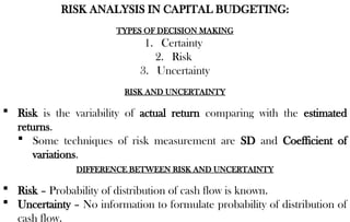
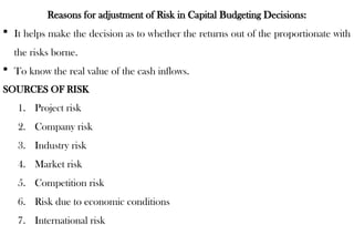
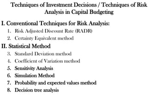
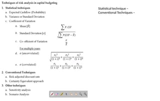
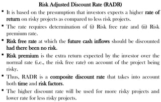
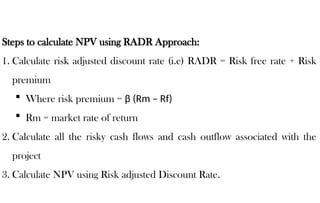
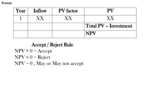
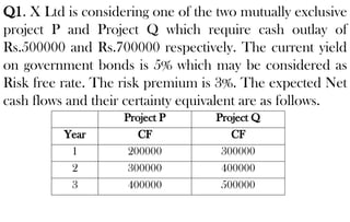
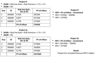
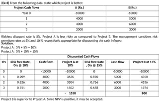
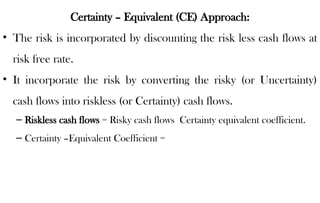
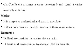
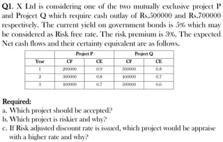
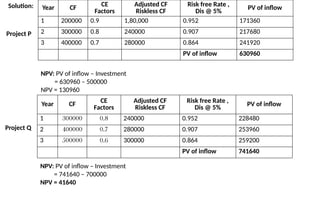
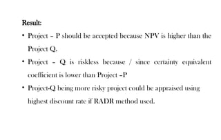
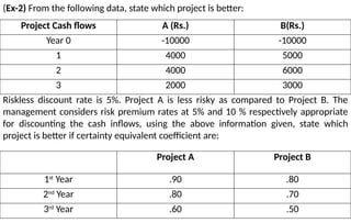
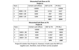
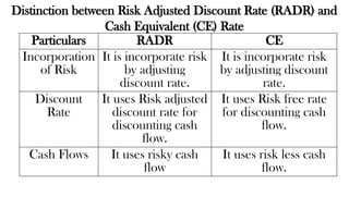
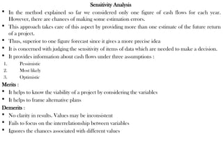
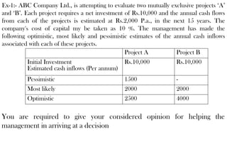
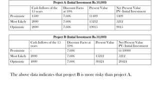
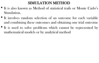
The document discusses advanced financial management focusing on risk analysis in capital budgeting, outlining the differences between risk and uncertainty, and various techniques for risk measurement such as the risk-adjusted discount rate and certainty equivalent method. It highlights the importance of adjusting for risk in capital budgeting decisions to assess the true value of expected cash inflows and includes examples of project evaluations. Additionally, it covers statistical methods for investment decisions including sensitivity analysis and simulation methods, along with their merits and demerits.

1. UNIT III: ADVANCED FINANCIAL
MANAGEMENT

2. RISK ANALYSIS IN CAPITAL BUDGETING:
TYPES OF DECISION MAKING
1. Certainty
2. Risk
3. Uncertainty
RISK AND UNCERTAINTY
 Risk is the variability of actual return comparing with the estimated
returns.
 Some techniques of risk measurement are SD and Coefficient of
variations.
DIFFERENCE BETWEEN RISK AND UNCERTAINTY
 Risk – Probability of distribution of cash flow is known.
 Uncertainty – No information to formulate probability of distribution of
cash flow.

3. Reasons for adjustment of Risk in Capital Budgeting Decisions:
 It helps make the decision as to whether the returns out of the proportionate with
the risks borne.
 To know the real value of the cash inflows.
SOURCES OF RISK
1. Project risk
2. Company risk
3. Industry risk
4. Market risk
5. Competition risk
6. Risk due to economic conditions
7. International risk

4. Techniques of Investment Decisions / Techniques of Risk
Analysis in Capital Budgeting
I. Conventional Techniques for Risk Analysis:
1. Risk Adjusted Discount Rate (RADR)
2. Certainty Equivalent method
II. Statistical Method
3. Standard Deviation method
4. Coefficient of Variation method
5. Sensitivity Analysis
6. Simulation Method
7. Probability and expected values method
8. Decision tree analysis

5. Statistical technique –
Conventional Techniques –

6. CONVENTIONAL TECHNIQUE
Risk Adjusted Discount Rate (RADR)
RADR is the discount rate which is used
to convert future cash inflow into
present values.
Certainty – Equivalent (CE) Approach:
The risk is incorporated by discounting
the risk less cash flows at risk free rate.

7. Risk Adjusted Discount Rate (RADR)
 It is based on the presumption that investors expects a higher rate of
return on risky projects as compared to less risk projects.
 The rate requires determination of (i) Risk free rate and (ii) Risk
premium rate.
 Risk free rate at which the future cash inflows should be discounted
had there been no risk.
 Risk premium is the extra return expected by the investor over the
normal rate (i.e., the risk free rate) on account of the project being
risky.
 Thus, RADR is a composite discount rate that takes into account
both time and risk factors.
 The higher discount rate will be used for more risky projects and
lower rate for less risky projects.

8. Merits :
It is easy to understand and very simple to calculate
It incorporate the risk averse attitude of investors.
Demerits :
 It may not give perfect results.
 It is to be adjusted and not the required rate of return.
 This method presumes that the risk necessarily increases with time
which may not be correct in all cases.
 This method presumes that the investors are averse to risk.
In spite of these disadvantages the method is most widely used on account of its
simplicity.

9. Steps to calculate NPV using RADR Approach:
1. Calculate risk adjusted discount rate (i.e) RADR = Risk free rate + Risk
premium
 Where risk premium = β (Rm – Rf)
 Rm = market rate of return
2. Calculate all the risky cash flows and cash outflow associated with the
project
3. Calculate NPV using Risk adjusted Discount Rate.

10. Format:
Year Inflow PV factor PV
1 XX XX XX
Total PV – Investment
NPV
Accept / Reject Rule
NPV > 0 = Accept
NPV < 0 = Reject
NPV = 0 , May or May not accept

11. Q1. X Ltd is considering one of the two mutually exclusive
project P and Project Q which require cash outlay of
Rs.500000 and Rs.700000 respectively. The current yield
on government bonds is 5% which may be considered as
Risk free rate. The risk premium is 3%. The expected Net
cash flows and their certainty equivalent are as follows.
Project P Project Q
Year CF CF
1 200000 300000
2 300000 400000
3 400000 500000

12. Year CF
Risk free Rate ,
Dis @ 8%
PV of inflow
1 200000 0.926 185200
2 300000 0.857 257100
3 400000 0.794 317600
PV of inflow 759900
Project P:
 RADR = Risk free Rate + Risk Premium = 5 % + 3 %
 RADR = 8%
Project P:
 NPV = PV of Inflow – Investment
 NPV =759900 – 500000
 NPV = 259900
Project Q:
 RADR = Risk free Rate + Risk Premium = 5 % + 3 %
 RADR = 8%
Year CF Risk free Rate ,
Dis @ 8%
PV of inflow
1 300000 0.926 277800
2 400000 0.857 342800
3 500000 0.794 397000
PV of inflow 1017600
Project Q:
 NPV = PV of Inflow – Investment
 NPV =1017600 – 700000
 NPV = 317600
Result
Project Q is accepted because NPV is higher

13. (Ex-2) From the following data, state which project is better:
Project Cash flows A (Rs.) B(Rs.)
Year 0 -10000 -10000
1 4000 5000
2 4000 6000
3 2000 3000
Riskless discount rate is 5%. Project A is less risky as compared to Project B. The management considers risk
premium rates at 5% and 10 % respectively appropriate for discounting the cash inflows:
Solution:
Project A: 5% + 5% = 10%
Project A: 5% + 10% = 15%
Discounted Cash Flows
Yrs Risk free Rate ,
Dis @ 10%
Cash flow Project A at
10%
Risk free Rate
, Dis @ 15%
Cash flow Project B at 15%
0 0 -10000 -10000 0 -10000 -10000
1 0.909 4000 3636 0.870 5000 4350
2 0.826 4000 3304 0.756 6000 4536
3 0.751 2000 1502 0.658 3000 1974
- 1558 860
Project B is superior to Project A. Since NPV is positive, it may be accepted.

14. Certainty – Equivalent (CE) Approach:
• The risk is incorporated by discounting the risk less cash flows at
risk free rate.
• It incorporate the risk by converting the risky (or Uncertainty)
cash flows into riskless (or Certainty) cash flows.
– Riskless cash flows = Risky cash flows Certainty equivalent coefficient.
– Certainty –Equivalent Coefficient =

15.  CE Coefficient assumes a value between 0 and 1,and it varies
inversely with risk
Merits :
 It is simple to understand and easy to calculate
 It does not consider the risk increase with increase in time
Demerits :
 Difficult to consider increasing risk capacity
 Difficult and inconvenient to allocate CE Coefficients.

16. Q1. X Ltd is considering one of the two mutually exclusive project P
and Project Q which require cash outlay of Rs.500000 and Rs.700000
respectively. The current yield on government bonds is 5% which may
be considered as Risk free rate. The risk premium is 3%. The expected
Net cash flows and their certainty equivalent are as follows.
Project P Project Q
Year CF CE CF CE
1 200000 0.9 300000 0.8
2 300000 0.8 400000 0.7
3 400000 0.7 500000 0.6
Required:
a. Which project should be accepted?
b. Which project is riskier and why?
c. If Risk adjusted discount rate is issued, which project would be appraise
with a higher rate and why?

17. Year CF CE
Factors
Adjusted CF
Riskless CF
Risk free Rate ,
Dis @ 5%
PV of inflow
1 200000 0.9 1,80,000 0.952 171360
2 300000 0.8 240000 0.907 217680
3 400000 0.7 280000 0.864 241920
PV of inflow 630960
Solution:
NPV: PV of inflow – Investment
= 630960 – 500000
NPV = 130960
Project P
Year CF CE
Factors
Adjusted CF
Riskless CF
Risk free Rate ,
Dis @ 5%
PV of inflow
1 300000 0.8 240000 0.952 228480
2 400000 0.7 280000 0.907 253960
3 500000 0.6 300000 0.864 259200
PV of inflow 741640
NPV: PV of inflow – Investment
= 741640 – 700000
NPV = 41640
Project Q

18. Result:
• Project – P should be accepted because NPV is higher than the
Project Q.
• Project – Q is riskless because / since certainty equivalent
coefficient is lower than Project –P
• Project-Q being more risky project could be appraised using
highest discount rate if RADR method used.

19. (Ex-2) From the following data, state which project is better:
Project Cash flows A (Rs.) B(Rs.)
Year 0 -10000 -10000
1 4000 5000
2 4000 6000
3 2000 3000
Riskless discount rate is 5%. Project A is less risky as compared to Project B. The
management considers risk premium rates at 5% and 10 % respectively appropriate
for discounting the cash inflows, using the above information given, state which
project is better if certainty equivalent coefficient are:
Project A Project B
1st
Year .90 .80
2nd
Year .80 .70
3rd
Year .60 .50

20. Years Certain cash inflows DCF @ 5% PV (Rs.)
0 -10000 -10000
1 4000 × .90 3600 0.952 3427
2 4000 × .80 3200 .907 2902
3 2000 × .60 1200 0.864 1037
NPV -2634
Discounted Cash flows at 5%
Project A
Discounted Cash flows at 5%
Project B
Years Certain cash inflows DCF @ 5% PV (Rs.)
0 -10000 -10000
1 5000 × .80 4000 0.952 3808
2 6000 × .70 4200 0.907 3809
3 3000 × .50 1500 0.864 1296
NPV -1087
Project B is better than Project A. However, in both cases the NPV is in
negative and , therefore, none of them can be accepted

21. Distinction between Risk Adjusted Discount Rate (RADR) and
Cash Equivalent (CE) Rate
Particulars RADR CE
Incorporation
of Risk
It is incorporate risk
by adjusting
discount rate.
It is incorporate risk
by adjusting discount
rate.
Discount
Rate
It uses Risk adjusted
discount rate for
discounting cash
flow.
It uses Risk free rate
for discounting cash
flow.
Cash Flows It uses risky cash
flow
It uses risk less cash
flow.

22. Sensitivity Analysis
 In the method explained so far we considered only one figure of cash flows for each year.
However, there are chances of making some estimation errors.
 This approach takes care of this aspect by providing more than one estimate of the future return
of a project.
 Thus, superior to one figure forecast since it gives a more precise idea
 It is concerned with judging the sensitivity of items of data which are needed to make a decision.
 It provides information about cash flows under three assumptions :
1. Pessimistic
2. Most likely
3. Optimistic
Merits :
 It helps to know the viability of a project by considering the variables
 It helps to frame alternative plans
Demerits :
 No clarity in results. Values may be inconsistent
 Fails to focus on the interrelationship between variables
 Ignores the chances associated with different values

23. Ex-1:- ABC Company Ltd., is attempting to evaluate two mutually exclusive projects ‘A’
and ‘B’. Each project requires a net investment of Rs.10,000 and the annual cash flows
from each of the projects is estimated at Rs.2,000 P.a., in the next 15 years. The
company's cost of capital my be taken as 10 %. The management has made the
following optimistic, most likely and pessimistic estimates of the annual cash inflows
associated with each of these projects.
Project A Project B
Initial Investment
Estimated cash inflows (Per annum)
Rs.10,000 Rs.10,000
Pessimistic 1500 -
Most likely 2000 2000
Optimistic 2500 4000
You are required to give your considered opinion for helping the
management in arriving at a decision

24. Project A (Initial Investment Rs.10,000)
Cash Inflows of the
15 years
Discount Facto
at 10%
Present Value Net Present Value
PV- Initial Investment
Pessimistic 1500 7.606 11409 1409
Most Likely 2000 7.606 15212 5212
Optimistic 2000 7.606 19015 9015
Project B (Initial Investment Rs.10,000)
Cash Inflows of the 15
years
Discount Facto at
10%
Present Value Net Present Value
PV- Initial Investment
Pessimistic - 7.606 (-) 10000
Most Likely 2000 7.606 15212 5212
Optimistic 4000 7.606 30424 20424
The above data indicates that project B is more risky than project A.

25. SIMULATION METHOD
 It is also known as Method of statistical trails or Monte Carlo’s
Simulation.
 It involves random selection of an outcome for each variable
and combining these outcomes and obtaining one trial outcome
 It is used to solve problems which cannot be represented by
mathematical models or by analytical method

26. DECISION TREE ANALYSIS
 Decision tree is a graphical representation of the relationship between a
present decision and future events, future decisions, and their
consequences in the form of branches of a tree.
 Evaluation of a project can be done in different stages and over a period of
years with the help of decision tree.
Merits :
 It is easy to understand and very simple
 Clearly brings out the assumptions and calculations
 Give an overview of all the possibilities – helps to keep the entire picture in mind
 Helps to analyze the assumptions in graphical form
Demerits :
 Time consuming
 Complex
 Difficult to make calculations when tree diagram become more complicated.