ACM Reference FormatSchumacher, C., Bickel, B., Rys, J., Mar.docx

ACM Reference Format
Schumacher, C., Bickel, B., Rys, J., Marschner, S., Daraio, C.,
Gross, M. 2015. Microstructures to Control
Elasticity in 3D Printing. ACM Trans. Graph. 34, 4, Article 136
(August 2015), 13 pages.
DOI = 10.1145/2766926 http://doi.acm.org/10.1145/2766926.
Copyright Notice
Permission to make digital or hard copies of all or part of this
work for personal or classroom use is granted
without fee provided that copies are not made or distributed for
profi t or commercial advantage and that
copies bear this notice and the full citation on the fi rst page.
Copyrights for components of this work owned
by others than the author(s) must be honored. Abstracting with
credit is permitted. To copy otherwise, or re-
publish, to post on servers or to redistribute to lists, requires
prior specifi c permission and/or a fee. Request
permissions from [email protected]
SIGGRAPH ‘15 Technical Paper, August 09 – 13, 2015, Los
Angeles, CA.
Copyright is held by the owner/author(s). Publication rights
licensed to ACM.
ACM 978-1-4503-3331-3/15/08 ... $15.00.
DOI: http://dx.doi.org/10.1145/2766926
Microstructures to Control Elasticity in 3D Printing
Christian Schumacher1,2 Bernd Bickel1,3 Jan Rys2 Steve
Marschner4 Chiara Daraio2 Markus Gross1,2
1Disney Research Zurich 2ETH Zurich 3IST Austria 4Cornell

University
Figure 1: Given a virtual object with specified elasticity
material parameters (blue=soft, red=stiff), our method computes
an assemblage of
small-scale structures that approximates the desired elastic
behavior and requires only a single material for fabrication.
Abstract
We propose a method for fabricating deformable objects with
spa-
tially varying elasticity using 3D printing. Using a single,
relatively
stiff printer material, our method designs an assembly of small-
scale microstructures that have the effect of a softer material at
the
object scale, with properties depending on the microstructure
used
in each part of the object. We build on work in the area of meta-
materials, using numerical optimization to design tiled
microstruc-
tures with desired properties, but with the key difference that
our
method designs families of related structures that can be
interpo-
lated to smoothly vary the material properties over a wide
range.
To create an object with spatially varying elastic properties, we
tile
the object’s interior with microstructures drawn from these
families,
generating a different microstructure for each cell using an
efficient
algorithm to select compatible structures for neighboring cells.
We

show results computed for both 2D and 3D objects, validating
sev-
eral 2D and 3D printed structures using standard material tests
as
well as demonstrating various example applications.
CR Categories: I.3.5 [Computer Graphics]: Computational Ge-
ometry and Object Modeling—Physically based modeling
Keywords: fabrication, topology optimization, 3D printing
1 Introduction
With the emergence of affordable 3D printing hardware and on-
line 3D printing services, additive manufacturing technology
comes
with the promise to make the creation of complex functional
phys-
ical artifacts as easy as providing a virtual description. Many
func-
tional objects in our everyday life consist of elastic, deformable
material, and the material properties are often inextricably
linked to
function. Unfortunately, elastic properties are not as easy to
control
as geometry, since additive manufacturing technologies can
usually
use only a single material, or a very small set of materials,
which
often do not match the desired elastic deformation behavior.
How-
ever, 3D printing easily creates complex, high-resolution 3D
struc-
tures, enabling the creation of metamaterials with properties
that

are otherwise unachievable with available printer materials.
Metamaterials are assemblies of small-scale structures that
obtain
their bulk properties from the shape and arrangement of the
struc-
tures rather than from the composition of the material itself. For
example, based on this principle, Lakes [1987] presented the
first
engineered materials that exhibit a negative Poisson’s ratio.
Since
then, numerous designs have been proposed, usually consisting
of
a periodic tiling of a basic pattern, and engineering their
structures
is an active area of research [Lee et al. 2012].
While designing a tiled microstructure to match given homoge-
neous material properties can be achieved with modest
extensions
to the state of the art, designing a complex microstructural
assem-
bly to achieve heterogeneous, spatially varying properties is
much
more challenging. We face a complex inverse problem: to deter-
mine a discrete small-scale material distribution at the
resolution
of the 3D printer that yields the desired macroscopic elastic
behav-
ior. Inverse problems of this type have been explored for
designing
periodic structures that can be tiled to synthesize homogeneous
vol-
umes, but the methods are computation-intensive and do not
scale
to designing non-periodic structures for objects with spatially

vary-
ing material properties.
Our goal is to enable users to employ metamaterials in their 3D
printing workflow, generating appropriate structures
specifically for
their available 3D printer model and base material within
seconds.
Clearly, designing entire models on the fly by directly optimiz-
ing over the whole structure is impractical. Instead, we propose
a
data-driven approach that efficiently assembles models out of
pre-
computed small-scale structures so that the result both
resembles
the desired local elasticity and also is within the capabilities of
the
available output device.
First, we precompute a database of tiled structures indexed by
their
elastic properties. We want these structures to cover a large and
ideally continuous region in the space of possible elastic
behaviors.
To achieve this goal, we introduce an optimization method for
sam-
pling structures that exhibit a range of desired behaviors, but
are
ACM Transactions on Graphics, Vol. 34, No. 4, Article 136,
Publication Date: August 2015
also sufficiently similar to allow interpolation. We initialize
this

optimization method either with a known structure or desired
elas-
tic property values, and then compute a family of similar
structures
that covers a subspace of possible elastic behaviors. We repeat
this
process, each time adding a new family of structures, to
increase
the coverage of the material space.
Second, to synthesize the metamaterials for a specific object,
we tile
the object’s interior with microstructures drawn from these
families.
Note that the same elastic behavior can be reproduced by
structures
that differ significantly in shape, and therefore the families
might
overlap in material space. This is an important feature of our
sys-
tem for reproducing spatially varying material behavior.
Spatially
neighboring structures must connect properly at their interface,
and
overlapping families provide us with a set of candidates for
each
tile, significantly increasing the chance of finding structures
com-
patible with neighboring tiles. We propose an efficient global
opti-
mization algorithm that selects an optimized tiling, taking into
ac-
count the need for neighboring structures to connect properly.
Our
final result is functional and 3D printable.

We evaluate our algorithm by fabricating several examples of
both
flat sheets and 3D objects with heterogeneous material
behavior.
For several isotropic and anisotropic 2D examples and isotropic
3D
examples, we measure the resulting elastic properties,
comparing
the actual material parameters to the values predicted by our
simu-
lation.
2 Related Work
Simulation and Homogenization Simulation of deformable ob-
jects has a long history in computer graphics [Nealen et al.
2006].
For accurate simulation of material behavior, the finite element
method is a popular choice, with a wide range of available
constitu-
tive models of materials. An excellent introduction can be found
in
Sifakis and Barbič [2012]. Inspired by the seminal work of
Hashin
and Shtrikman [1963], homogenization theory was developed to
ef-
ficiently simulate inhomogeneous materials with fine structures,
al-
lowing microscopic behavior to be averaged into a coarser
macro-
scopic representation with equivalent behavior at the
macroscopic
scale [Michel et al. 1999; Cioranescu and Donato 2000]. Nesme
et al. [2009] encode the material stiffness within coarse
elements
using shape functions after a fine-level static analysis. We build

on the numerical coarsening approach by Kharevych et al.
[2009]
which turns the heterogeneous elastic properties represented by
a
fine mesh into possibly anisotropic elastic properties of a coarse
mesh that effectively captures the same physical behavior. After
computing harmonic displacements to capture how the fine
mesh
behaves, their approach presents an analytic relationship
between
the elasticity tensors of a coarse element and the elasticity
tensors
of the fine elements contained within. We extend this
formulation
for inverse homogenization.
Mechanical Metamaterials and Inverse Homogenization
Metamaterials are usually defined as macroscopic composites
having a manmade, periodic cellular architecture designed to
produce a behavior not available in nature. In this paper, we
draw
inspiration from mechanical metamaterials, and relax the term
in
the context of 3D printing to material properties not available
on
3D printers. Lakes [1987] presented the first engineered
materials
that exhibit a negative Poisson’s ratio. Due to their structure,
these
materials expand laterally when stretched, therefore increasing
their volume. Since then, numerous designs for soft
metamaterials
have been proposed, either found by intuition, or numerical
optimization processes [Lee et al. 2012].
In classical inverse homogenization approaches the goal is to

find
a repetitive small-scale structure with desired macroscopic
prop-
erties. This is obtained by optimizing the material distribution
in the base cell. Researchers have proposed various
parametriza-
tions of the material distribution, such as networks of bending
beams [Hughes et al. 2010], spherical shells patterned with an
ar-
ray of circular voids [Babaee et al. 2013], or rigid units [Attard
and Grima 2012]. Alternatively, the domain of a base cell can
be
discretized into small material voxels, and a discrete value
prob-
lem has to be solved. Due to the combinatorial complexity, di-
rect search methods are prohibitively expensive, and the
problem
is usually solved using a relaxed formulation with continuous
ma-
terial density variables [Sigmund 2009] or advanced search
heuris-
tics [Huang et al. 2011]. These approaches generally search for
structures with extreme properties, often maximum stiffness, for
a
given amount of material, and only consider a single structure.
In
contrast, we present an optimization method that computes a
struc-
ture to achieve a specific material behavior. Based on this
method,
we span an entire space of elastic material structures, and
construct
a mapping from elasticity parameters to microstructures that can
be
efficiently evaluated during runtime.

Rodrigues et al. [2002] and Coelho et al. [2008] suggest
methods
for hierarchical topology optimization, computing a continuous
ma-
terial distribution on a coarse level and matching
microstructures
for each coarse cell. While in their approach each
microstructure
cell can be optimized independently, each of them still needs to
be
computed based on a costly optimization scheme, and there is
no
guarantee on the connectivity of neighboring structures. In con-
trast, we use a data-driven approach which allows us to synthe-
size structures extremely efficiently, and also take the quality of
the connectivity into account. For functionally graded materials
with microstructures, Zhou et al. [2008] guarantee the matching
of
boundaries either by prescribing connectors or by incorporating
a
complete row of cells that form a gradient during a single
optimiza-
tion. We follow a different strategy. Instead of restricting types
of
connections or increasing the size of structures, we efficiently
com-
pute multiple candidates from families of microstructures and
then
select structures with interfaces that match best.
Fabrication-Oriented Material Design In computer graphics,
we are currently witnessing an increasing interest in
fabrication-
oriented material design for reproducing 3D physical artifacts
from

virtual representations. Recently, Chen et al. [2013] presented
an
abstraction mechanism for translating functional specifications
to
fabricable 3D prints, and Vidimče et al. [2013] introduced a
pro-
grammable pipeline for procedural evaluation of geometric
detail
and material composition, allowing models to be specified
easily
and efficiently. For static objects, Zhou et al. [2013] present an
al-
gorithm for efficiently analyzing the structural strength, and
Stava
et al. [Stava et al. 2012] improve the structural strength by
auto-
matic hollowing, thickening, and strut insertion. Wang et al.
[Wang
et al. 2013] propose a method for computing skin-frame
structures
for the purpose of reducing the material cost of the printed
object.
Recent work also investigated the reproduction of appearance,
for
example by modulating the surface structure to achieve desired
re-
flection properties [Weyrich et al. 2009; Lan et al. 2013;
Rouiller
et al. 2013], by interleaving different colored materials on the
sur-
face [Reiner et al. 2014], or by volumetric combination of
multiple
materials [Hašan et al. 2010; Dong et al. 2010] to control
subsurface
scattering behavior. Conceptually similar to our approach, these

methods are based on the principle that the large-scale
appearance
is governed by small-scale details, and can reproduce
appearance
properties which are significantly different from the 3D
printer’s
base material.
Bickel et al. [2010] presented a data-driven process for
designing
136:2 • C. Schumacher et al.
pre-process: metamaterial family construction run-time:
synthesis
microstructure
optimization
material space
sampling
input material
parameters
microstructure
synthesis
tiling
optimization

output
printable model
database: metamaterial space
Figure 2: An overview of our system. In a pre-processing step,
we compute metamaterial families. Each family consists of
multiple related
microstructures that can be interpolated to smoothly vary the
material properties. We store all families in a database,
representing our
metamaterial space. Given as input an object with specified
material parameters, we synthesize locally microstructures that
resemble the
desired deformation behavior. As multiple, topologically
different structures can have the same bulk behavior, we
potentially have multiple
candidates of microstructures for a single location. Using these
candidates, we compute an optimized tiling, ensuring that
neighboring
structures are properly connected. Finally, the physical
prototype is 3D printed.
and fabricating objects with desired deformation behavior.
Whereas
Bickel et al. start from specified example deformations, the
input
to our system is a model with specified elastic parameters. Their
approach assumes that a small set of microstructures is already
given, and finds a discrete combination of stacked layers from
these
structures that meets the criteria specified by the example
deforma-
tions. In contrast, our work computes the small-scale structures
themselves. This is essential for more precise local control of
the

deformation. Furthermore, Bickel et al. select a material for
each
layer using a branch-and-bound discrete optimization operating
on
the exponential space of designs, requiring running times on the
order of an hour for examples with five layers and nine base
materi-
als. By contrast, our method synthesizes the desired structures
from
pre-computed continuous material subspaces, and is able to
handle
objects with thousands of layers or cells within seconds.
Several previous methods investigate fitting spatially varying
ma-
terial parameters either from measurements of real-world ob-
jects [Becker and Teschner 2007], infer them from user-
specified
input such as example deformation [Skouras et al. 2013], or op-
timize material distributions to achieve higher-level
functionality
such as locomotion of soft robots [Hiller and Lipson 2012]. Re-
cently, Xu et al. [2015] presented an interactive material design
tool, which computes a spatial distribution of material
properties
given user-provided displacements and forces at a set of mesh
ver-
tices. Our method complements these approaches, working
towards
the goal of automatically converting the virtual representation
ob-
tained by those methods into 3D printable objects.
3 Overview
The goal of our system is to automatically convert an object

with
given spatially varying elastic properties into a 3D printable
rep-
resentation that requires only a single base material for fabrica-
tion, and mimics the desired elastic behavior. In this work, we
limit ourselves to small strains and demonstrate our approach
for
both isotropic and anisotropic elastic materials. As outlined in
Figure 2, our system consists of two main stages: a preprocess-
ing step that constructs metamaterial structures covering the
space
of reproducible material properties, and a synthesis stage that
uses
those structures to generate microstructures for a given object.
We
start the description by defining the most important terms we
use
throughout the paper.
Metamaterial Space A metamaterial space is a specific organi-
zation of metamaterials. We target reproducing elastic behavior
us-
ing 3D printers and represent their behavior using the n
parameters
of the underlying constitutive model. For example, linear
isotropic
materials are represented by n = 2 parameters, the Young’s
mod-
ulus and Poisson’s ratio. In addition, every metamaterial space
has
a mapping function, mapping the n parameters to one or several
microstructures. This mapping is one-to-many because different
microstructures might reproduce the same elastic behavior.
Metamaterial Space Construction Our first stage aims to de-

fine a function that efficiently maps a given elastic material to a
small, tileable structure with the same bulk behavior. Our
process
starts by systematically sampling the material parameter space.
Our
strategy is to compute a sparse set of representative structures
that
(i) cover a wide range in the space of elastic material
parameters
and that (ii) allow the interpolation of neighboring structures in
pa-
rameter space. Via a weighted combination of these samples, we
then reconstruct a continuous mapping from elasticity
parameters
to microstructures. We call such a set of interpolatable
structures
a metamaterial family. A metamaterial family defines a one-to-
one
mapping from material properties to structure. In practice, a
family
usually only covers a partial gamut of the material space.
Therefore,
we pre-compute several families until we sufficiently cover a
de-
sired range of elastic behavior. All metamaterial families
together
constitute our metamaterial space. Note that, as shown in Figure
10,
the gamut of these metamaterial families might be partially
over-
lapping, yielding a one-to-many mapping from parameters to
mi-
crostructures.
Synthesis To synthesize the microstructure for a given object,
we tile its interior. For each tile, we interpolate a microstructure

from each pre-computed family of structures. This provides us
with
a small set of candidate structures for each cell, out of which we
have to select exactly one. These choices are not independent;
they
must be made consistently so that the structures connect well
with
their neighboring tiles. We suggest a carefully designed metric
that
quantifies the compatibility of structures and phrase this
selection
as a combinatorial problem, which we solve efficiently using an
optimization method based on message passing. Finally, we use
the
selected structures to fabricate the object using rapid
prototyping.
4 Background
In order to determine and optimize for the behavior of a
microstruc-
ture, a physical model is introduced. This model combines
standard
linear elasticity with extensions specific to microstructure
simula-
tion and topology optimization.
4.1 Linear Elasticity
Continuum mechanics in combination with a finite elements dis-
cretization is a popular way to model elastic structures. For
stan-
Microstructures to Control Elasticity in 3D Printing •
136:3

dard linear elasticity, the energy density can be defined as
W = ε : C : ε = ε : σ. (1)
Here, ε is the linear Cauchy strain, C is the material stiffness
ten-
sor, and σ = C : ε is the Cauchy stress tensor. The material
stiffness tensor is defined by a small set of parameters that
depend
on the material model. For example, for an isotropic material, it
is a function of 2 parameters, the Young’s modulus and the
Pois-
son’s ratio. For more complex materials, additional parameters
such
as the shear modulus and direction-dependent Young’s moduli
and
Poisson’s ratios are used. Given parameters p, we denote the
cor-
responding material stiffness tensor as C(p).
A linear finite element method is used to discretize (1) with
basis
functions defined on triangular and tetrahedral elements in 2D
and
3D, respectively. In this case, the strain εi and material stiffness
tensor Ci are constant within an element i. The elastic energy,
given as the volume integral of the energy density, is then
Uel =
k∑

i=1
(εi : Ci : εi) Vi (2)
for a model with k elements and element areas/volumes Vi. The
to-
tal energy of the system also considers external forces and
tractions.
Summarizing surface traction and forces using a general force
field
f acting on vertices, this energy can be expressed as
Utot(x) = Uel(x) −
n∑
i=1
x
T
i fi, (3)
where n is the number of vertices, and vector x =
[
xT1 · · ·xTn
]T
is the concatenation of all vertex position vectors. The
deformed
configuration x corresponding to the static equilibrium can be
com-
puted by minimizing this energy, or equivalently, solving
∇ xUel(x) = f. (4)
Since the elastic energy Uel(x) is invariant to translation and
rota-

tion, the solution to this problem is not unique. A common
work-
around to this is to constrain enough degrees of freedom to get
rid
of this nullspace. However, the choice of degrees of freedom
might
influence the solution in the presence of forces. Instead, we opt
to
resolve the ambiguities by introducing constraints on the
moments
of the object, similar to Zhou et al. [2013]. These constraints
take
the form
c1(x) =
n∑
i=1
(xi −Xi) = 0
c2(x) =
n∑
i=1
((xi −Xi) × (xi −X)) = 0,
(5)
where Xi is the rest state position of vertex i, and X is the mean
rest state position. For simplicity, we combine these constraints
into a single vector c(x) = [c1(x)T c2(x)T ]T . Intuitively, these
constraints fix the mean translation and rotation. To compute c2
in
the 2D case, we treat positions as points on the z = 0 plane and
use

the z-component of the cross product.
Combining Equation (4) and Equation (5), the problem of
comput-
ing the equilibrium configuration then becomes
∇ xUel(x) = f s.t. c(x) = 0. (6)
This problem can be expressed as a system of linear equations
and
solved efficiently.
4.2 Microstructure Simulation
The simulation of a microstructure can be simplified by
consider-
ing a tiling of a representative base cell. Instead of simulating
the
complete tiling to determine the behavior of the structure,
periodic
boundary conditions can be added to a simulation of a single
cell.
These boundary conditions simulate the tiling and essentially
re-
quire that opposite boundaries of the cell have the same shape.
x1
base
x0
base
xi
xj
free vertex

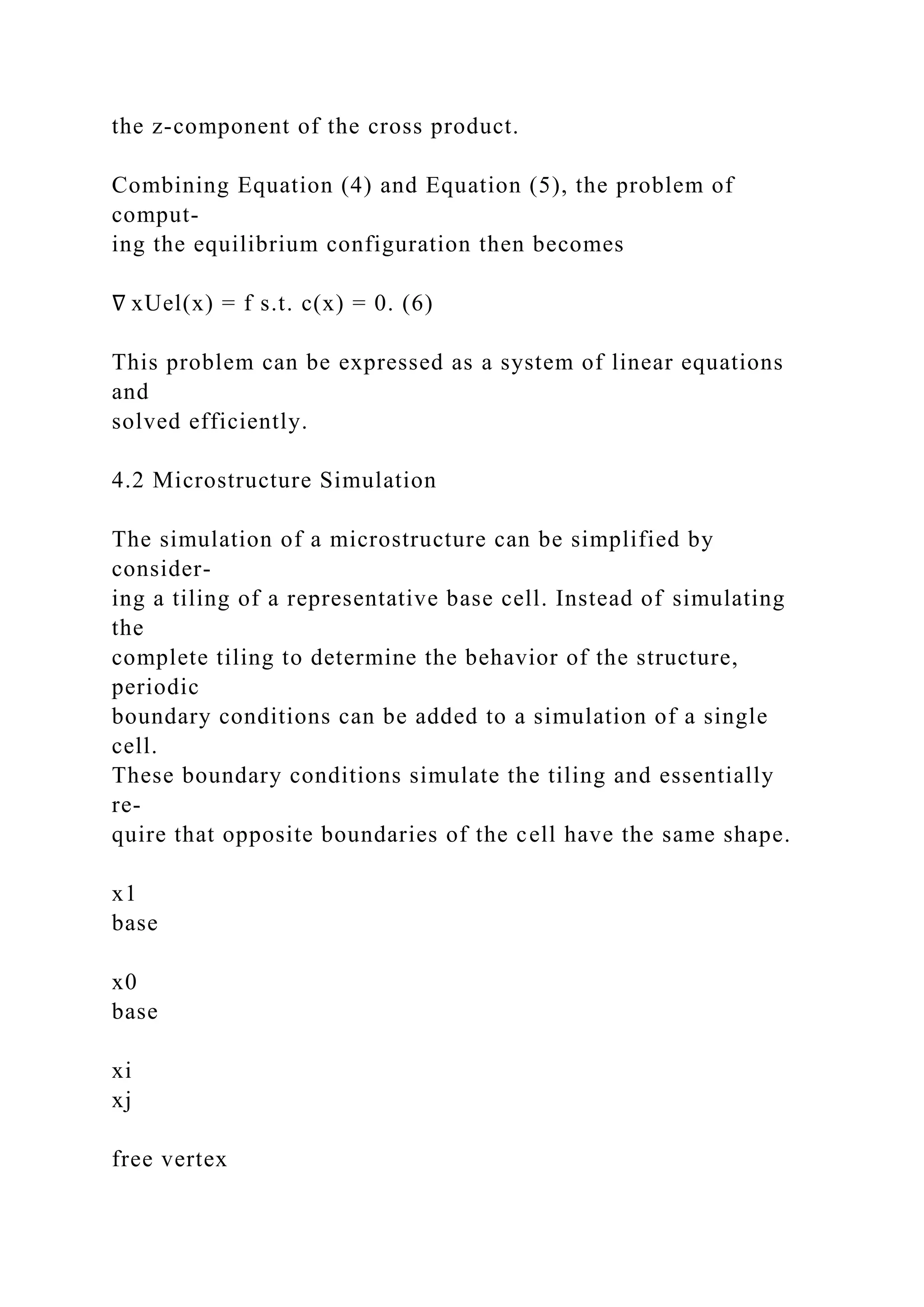
constrained vertex
Specifically, we assume that any vertex
on a boundary has a matching vertex on
the opposite boundary such that its rela-
tive position on the boundary is identical.
Choosing an arbitrary pair of boundary
vertices xbase0 and x
base
1 as base vertices
then defines the distance between two op-
posite boundaries, and any other vertex
xj on one boundary can be expressed as
a combination of the base vertices and the
corresponding vertex xi on the opposite
boundary [Smit et al. 1998]
xj = x
base
1 + xi −x
base
0 . (7)
These boundary conditions can be efficiently integrated into a
sim-
ulation by removing the corresponding vertices from the degrees
of
freedom.
4.3 Numerical Coarsening
Optimizing a microstructure is an inverse problem,
corresponding

to the forward problem of determining the coarse-scale behavior
from the microstructure. This forward problem can be defined
us-
ing the idea of homogenization: compute a material stiffness
tensor
for a homogeneous material whose elastic behavior matches that
of the tiled microstructure. We use the Numerical Coarsening
ap-
proach [Kharevych et al. 2009], which uses a set of load cases
to
approximate the coarse elastic behavior of a given structure.
Essen-
tially, given the deformations h that these load cases induce,
which
are called harmonic displacements, the method computes a
single
material stiffness tensor C(h) that describes the homogenized
ma-
terial behavior of a microstructure, which we will use to solve
the
inverse problem. We refer to the supplemental material for a de-
tailed introduction to the Numerical Coarsening approach.
5 Microstructure Optimization
Our microstructure optimization method solves the inverse
problem
to the Numerical Coarsening method mentioned in the previous
sec-
tion, solving for a microstructure that coarsens to a given
stiffness
tensor.
Optimizing a microstructure requires a way to define and alter
the
material distribution within a cell. A common approach in

topology
optimization is to discretize the material distribution by
subdivid-
ing the cell into a grid of material voxels [Sigmund 2009],
where
each voxel is associated with a binary activation that describes
whether the voxel is full (1) or void (0). However, optimizing
the
microstructure using these binary variables directly would be
in-
feasible for moderately large grids. Instead, the problem is
usually
relaxed by allowing the activations to vary smoothly between 0
and
1 during the optimization, and only requiring them to converge
to
a binary solution at the end of the optimization. For the
continuous
activations, a meaningful interpolation between void and full
voxels
has to be defined such that the activation corresponds to a
physical
quantity in the simulation. A simple way to define this is by
inter-
polating between stiffness tensors. For any voxel i (1 ≤ i ≤ m,
with m being the number of voxels), an individual material
stiffness
tensor Ci is defined as an interpolation between the base

material
stiffness tensor Cbase and air, which is assumed to have a zero
ma-
terial stiffness tensor:
Ci = αiCbase. (8)
To ensure numerical stability, the minimum of αi is set to αmin
=
10−5. This interpolation scheme follows the established SIMP
(solid isotropic material with penalization) approach for an
expo-
nent of 1 [Sigmund 2009]. Choosing a different exponent would
help to converge to a binary solution in topology optimization
prob-
lems with extremal objectives, where adding more material im-
proves the objective and the maximum amount of material is
fixed
by a constraint. However, we do not have such an objective, and
have to resort to other means to reach a binary solution. As a
con-
sequence, the exponent we choose does not influence the
conver-
gence.
The number of activations can be reduced by exploiting
symmetries
of the goal material. For example, for a cubic material, the
response
along each axis has to be identical. Mirroring the activations
along
all axes and all diagonal planes will therefore not constrain the
so-
lution.
5.1 Problem Formulation

We pose the problem of finding a microstructure that exhibits a
large-scale behavior identical to a homogeneous material with
de-
sired material parameters pgoal (see Section 4.1) as a least
squares
problem. From the parameters pgoal, a stiffness tensor Cgoal =
C(pgoal) can be computed. The optimization then modifies the
ac-
tivations α such that the homogenized stiffness tensor C(h(α)),
which is indirectly dependent on the activations through the
har-
monic displacements h(α), matches the goal stiffness tensor as
closely as possible:
min
α
‖Cgoal −C(h(α))‖2F + R
s.t. αmin ≤ αi ≤ 1 1 ≤ i ≤ m.
(9)
Here, R is a combined regularization term that penalizes less
desir-
able results. This formulation differs from most other
microstruc-
ture optimization approaches that typically try to find extremal
properties for a specific amount of material. It is related to the
formulation in [Zhou and Li 2008], though it does not use a
volume
fraction constraint.
5.2 Regularization
While the optimization problem (9) could be solved without any

regularization, there is no guarantee that the result can be fabri-
cated. In order to enforce manufacturability, we add three
different
regularization terms Rint, Rs and Rcb with corresponding
weights
wint, ws and wcb to the objective. The combined regularization
term
R is defined as
R = wintRint + wsRs + wcbRcb. (10)
Figure 3 and 4 show the influence of the individual
regularization
terms. In the following, we will elaborate on each term.
Enforcing Integer Values While the simulation allows the acti-
vations α to vary freely between αmin and 1, these
configurations do
not correspond to valid physical objects. For fabrication, the
activa-
tions have to be integral (excluding the small offset αmin to
ensure
stability). In order to reach such a solution, the regularization
term
Rint acts as a penalty for activations that are not equal to either
αmin
or 1:
Rint =
m∑
i=1
(αi −αmin) (1 −αi) . (11)

We gradually increase the weight wint during the optimization,
tran-
sitioning from a continuous to a discrete solution. For each
value of
the weight, a full optimization is run until convergence is
reached.
If the solution is not binary, the weight is increased and the op-
timization resumed. Figure 3 and the accompanying video show
different stages of the optimization, with various weights wint.
wint = 7.49 wint = 11.33 wint = 87.38 wint = 3.2 · 1012
Figure 3: Optimization at different stages (with different
penalty
weights to force the activations towards αmin or 1).
Smoothness The size of a single microstructure cell in a fab-
ricated object is largely defined by two factors: the resolution
of
the 3D printer, and the size of the smallest detail in the
structure.
Smaller cells provide a better approximation of a continuous
mate-
rial, and since the printer resolution is assumed to be fixed,
struc-
tures without small details are generally preferred.
The regularization Rs views the activations as an approximation
of a material distribution field, and uses a second-order finite
dif-
ference approach to penalize deviations from smoothness. For
this
purpose, any component of α is assumed to have two indices in
2D, such that αi,j corresponds to the voxel (i,j). The regulariza-
tion then has the form

Rs =
∑
i,j
(αi−1,j + αi+1,j + αi,j−1
+αi,j+1 − 4αi,j )2
(12)
in 2D; the formula for the 3D case is similar and can be found
in
the supplemental document.
136:5
Rint Rint + Rcb Rint + Rcb + Rs
Figure 4: Influence of different regularizations: Optimization
re-
sults where only integer values are enforced (left), with addi-
tional anti-checkerboard regularization (middle) and with
smooth-
ness regularization (right). The objective value for the last two
re-
sults is similar, while the first result has a worse objective
value.
Checkerboard Patterns An artifact that frequently appears in
topology optimization is elements that are connected by a sin-
gle vertex, called checkerboard patterns [Sigmund and Petersson

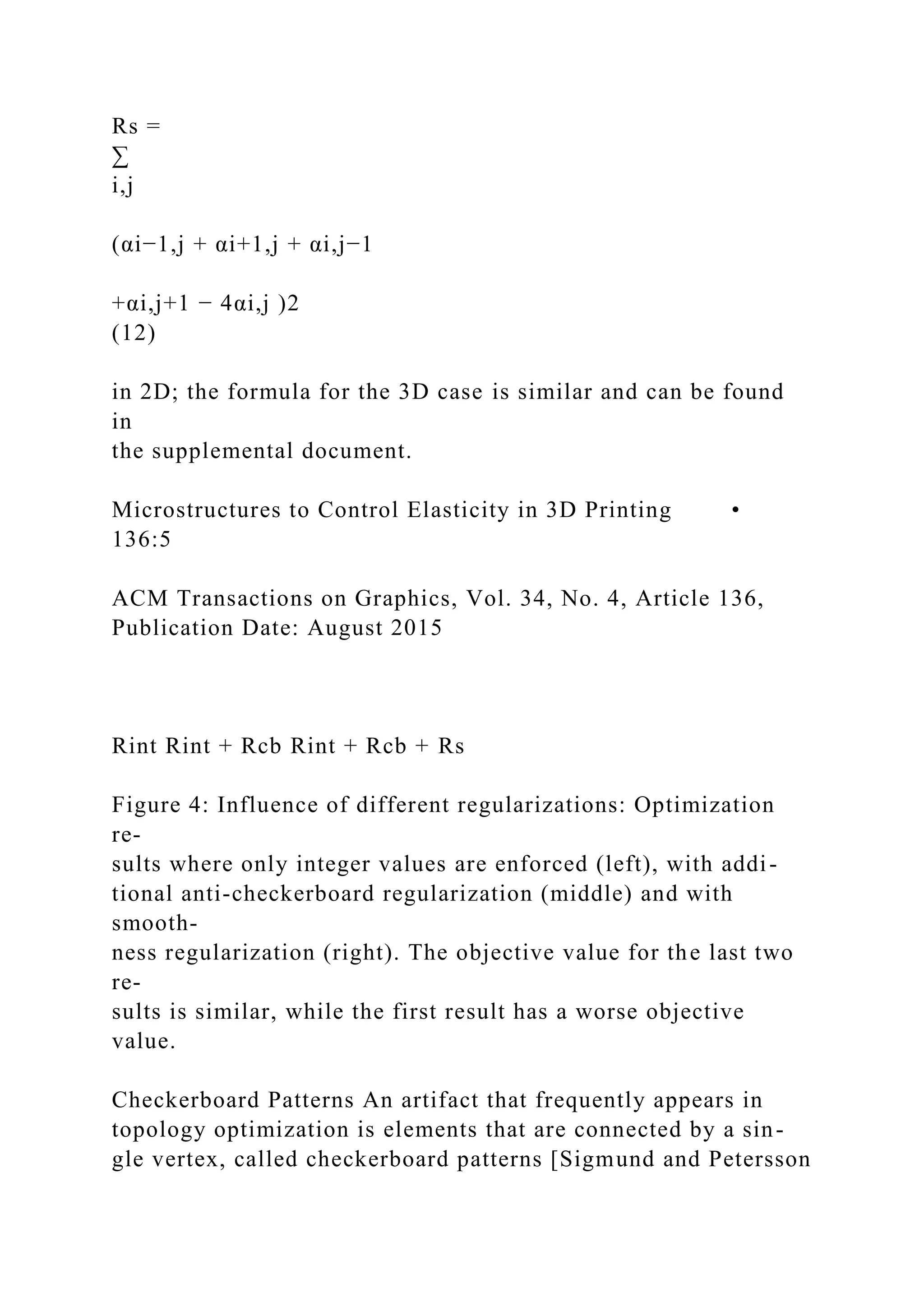
1998]. To avoid such structures, the regularization Rcb
penalizes
configurations that contain checkerboard patterns, as illustrated
in
Figure 4. In 2D, this regularization is based on 2 × 2 patches of
voxels and has the form
Rcb =
∑
i,j
(1 −αi,j )(αi+1,j −αmin)
(αi,j+1 −αmin)(1 −αi+1,j+1)
+(αi,j −αmin)(1 −αi+1,j )
(1 −αi,j+1)(αi+1,j+1 −αmin).
(13)
In the case of binary activations, Rcb is only non-zero if the
struc-
ture contains a checkerboard pattern. In the continuous case, the
regularization also acts as an additional regularizer that pushes
the
activations towards αmin or 1.
In 3D, the number of different local checkerboard patterns in-
creases. The corresponding formula can be found in the supple-
mental document.
Regularization Weights The performance of our microstructure
optimization depends on the choice of weights, and how they
are
updated during the optimization. For the optimization in 2D, we
start with w0int = 0, w

0
s = 2 and w
0
cb = 0. Once the optimization
converged for the current weights, we update them according to
wt+1int = 1.3w
t
int + 0.1, w
t+1
s = 1.1w
t
s + 0.2 and w
t+1
cb = 5w
t+1
int ,
until a final solution has been found. In 3D, we initialize the
weights
with w0int = 0, w
0
s = 5 and w
0
cb = 0, and update them using
wt+1int = 1.3w

t
int + 0.5, w
t+1
s = 1.1w
t
s + 1 and w
t+1
cb = 5w
t+1
int .
Connectivity An additional fabrication requirement is
connectiv-
ity. The optimization will generally not favor binary solutions
in
the absence of regularization term Rint. As the influence of this
term grows with increasing wint, the previously intermediate
activa-
tions will be pushed to αmin or 1, and the structure might
become
disconnected (see Figure 5). To prevent the optimization from
con-
verging to such a solution, disconnected components are
detected
after every iteration. To account for the continuous nature of the
activations, every activation below a threshold of 0.1 is
considered
inactive during the detection. If a disconnected component has
been
found, we compute the cost of connecting the component as the
smallest change in activations that builds a connection,
assuming

that we set the activations to a value of 0.6. If this cost is
smaller
than the change in activations necessary to remove the
disconnected
(a) (b) (c) (d)
Figure 5: Influence of the connectivity enforcement: Without
using
any connectivity enforcment during the optimization (a), the
final
structure might consist of several disconnected components (b).
En-
forcing connectivity with our scheme locally adjusts the
activations
(c) such that the final result is guaranteed to be fully connected
(d).
component, we create the connection, and remove the
disconnected
component otherwise. The final result is then guaranteed to be
con-
nected.
In 3D, an additional fabrication constraint is necessary. While
3D
printing can handle complex structures, most approaches rely on
support material to create overhanging structures. This support
ma-
terial has to be removed after printing. This means that every
void
voxel in the structure has to be connected to the boundary of the
cell. To this end, we use the same approach we used to connect
components, but switch the role of void and full voxels. In prac-
tice, we did not observe any convergence problems due to these
constraints.

5.3 Numerical Methods
The optimization problem (9) is solved with L-BFGS-B [Byrd
et al. 1995], which enforces the boundary constraints. Addition-
ally, the indirect relationship between the coarsened stiffness
tensor
C(h(α)) and the activations α through Numerical Coarsening has
to be taken into account when computing the gradient of the ob-
jective. We refer to the supplemental document for details on
this
computation.
6 Metamaterial Spaces
The optimization method from the previous section is able to
pro-
duce microstructures for a variety of material parameters, but
may
take a long time to generate a desired structure. Moreover, if the
de-
sired object contains spatially varying parameters, several
optimiza-
tions need to be performed to generate the required
microstructures,
making this approach infeasible in practice. To avoid this
problem,
we use a data-driven approach to assemble a structure with a de-
sired behavior by interpolation from a pre-computed
metamaterial
family.
A metamaterial family is a collection of microstructures, each
labeled with its corresponding coarse-scale material parameters,
which are a point in the space of possible material properties
(pa-

rameter space); we think of the microstructure as being “located
at”
that point. In this section, we first describe how the structures
are
represented and how their locations in parameter space are
deter-
mined. We then propose a technique to interpolate between
these
structures, providing a way to efficiently compute a
corresponding
microstructure for any point in the parameter space. Finally, we
discuss how to use the microstructure optimization approach de-
scribed in the previous section to create metamaterial families
by
computing sets of related microstructures that cover a wide
range
in parameter space.
In Section 7 we explain how several such continuous families
(col-
lectively, a metamaterial space) are used together to assemble
mod-
els spanning the entire range of achievable material properties.
6.1 Microstructure Representation
Geometry While the voxel-based discretization we used during
the microstructure optimization is useful in that context, it

poses
two problems for the construction of a metamaterial space: (i)
The
changes to the structure are all discrete in nature, so the
resulting
interpolation cannot be continuous, and (ii) the resulting
geometry
can contain stair structures. These sharp corners can lead to lo-
calized stresses under deformation and the structure would
fracture
more easily.
Instead of using voxels, we use signed L2-distance fields in [0,
1]d
to represent structures in a metamaterial space, which allows for
a
smooth interpolation. Additionally, we perform a Gaussian
smooth-
ing step every time we sample a microstructure from the
metama-
terial space, which removes unwanted discretization artifacts
(Fig-
ure 6). To increase resolution, we scale the grid resolution by a
factor of 2 and 3 compared to the original voxelization, in 2D
and
3D, respectively.
Material Parameters Numerical Coarsening is used to compute
a stiffness tensor that describes the behavior of a particular mi-
crostructure. However, for sampling and interpolation we would
like to use a parameter space with fewer degrees of freedom
than
this tensor has (6 in two dimensions, 21 in three dimensions).
By
considering only isotropic, cubic or orthotropic materials, the

pa-
rameter space can be reduced to a subset of material tensors,
while
still offering enough freedom to show a large variety of
deformation
behaviors.
To approximate the parameters from a material stiffness tensor
computed by Numerical Coarsening, a simple constrained least-
squares approach is used. Assuming a material stiffness tensor
Ĉ
is given, the corresponding parameters are computed by solving
min
p
‖C(p) − Ĉ‖2F
s.t. pmini ≤ pi ≤ p
max
i .
(14)
The function C(p) is defined by the choice of the material
model,
and pmini and p
max
i are the physics-based bounds on the parameters,
such as the lower limit of 0 for the Young’s modulus. We addi-
tionally apply a normalization to the parameters that transforms
all
parameters with dimensions, such as the Young’s modulus or
the
shear modulus, into dimensionless parameters by dividing them

by
the corresponding parameter of the base material. Since we use
a
linear material model, the resulting parameters describe the
ratio
of the structure’s parameter to the base material’s parameter,
which
also allows us to scale our results to materials with an arbitrary
σ = 0 σ = 0.005 σ = 0.02 σ = 0.05
Figure 6: Results of the smoothing pass for different Gaussian
spread values σ.
w = 0.25 w = 0.50 w = 0.75
Figure 7: Top row: Results of the interpolation between the
struc-
tures on the left and right for different weights w. Bottom row:
Cor-
responding signed distance fields, illustrated as color plots
(blue
positive, red negative).
Young’s modulus or shear modulus, assuming that the Poisson’s
ra-
tio stays the same. Additionally, since we use this relative
Young’s
modulus and relative shear modulus to store entries in
parameter
space, the distance between the parameters of two
microstructures
is independent of the base material’s stiffness.
6.2 Interpolation

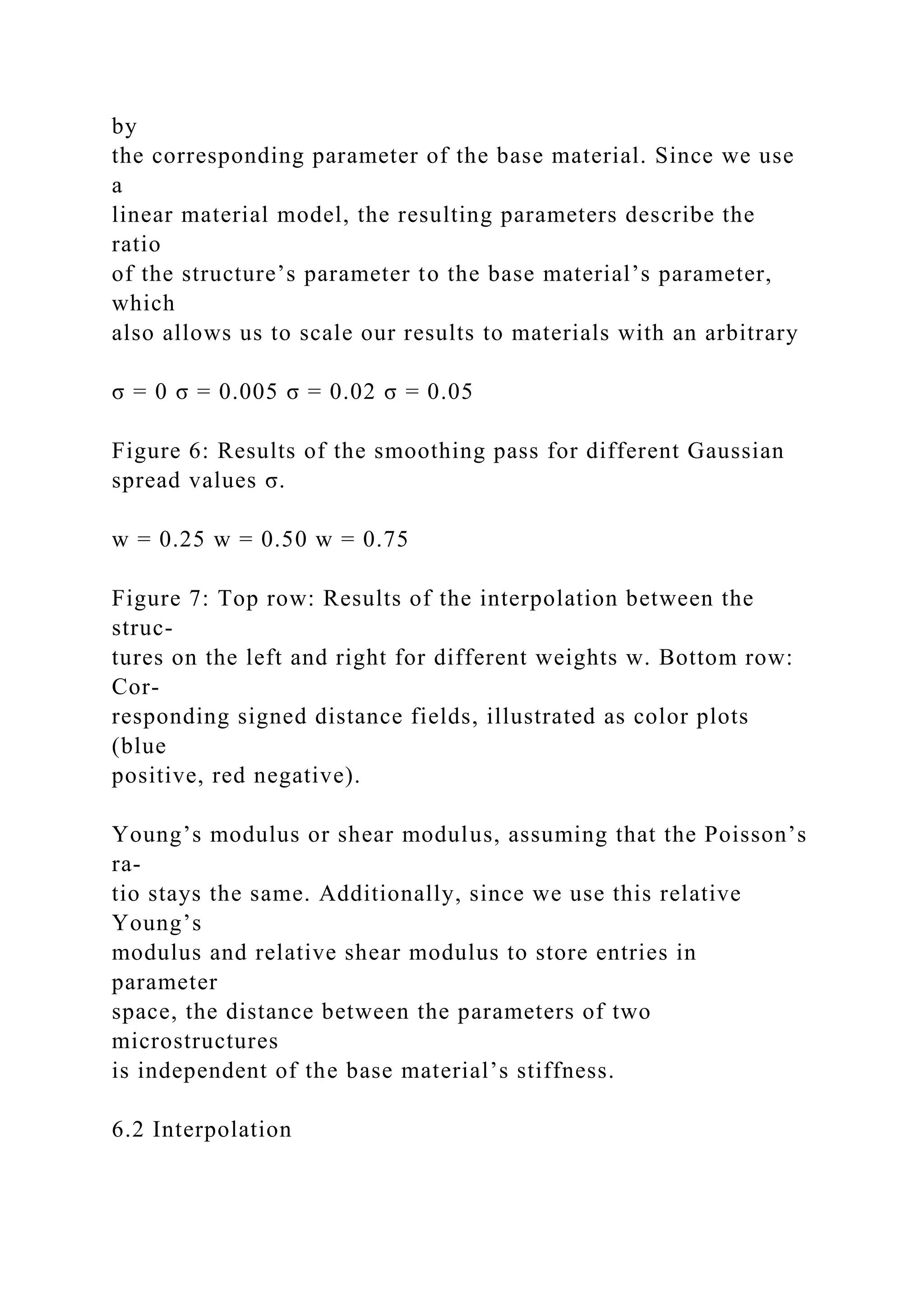
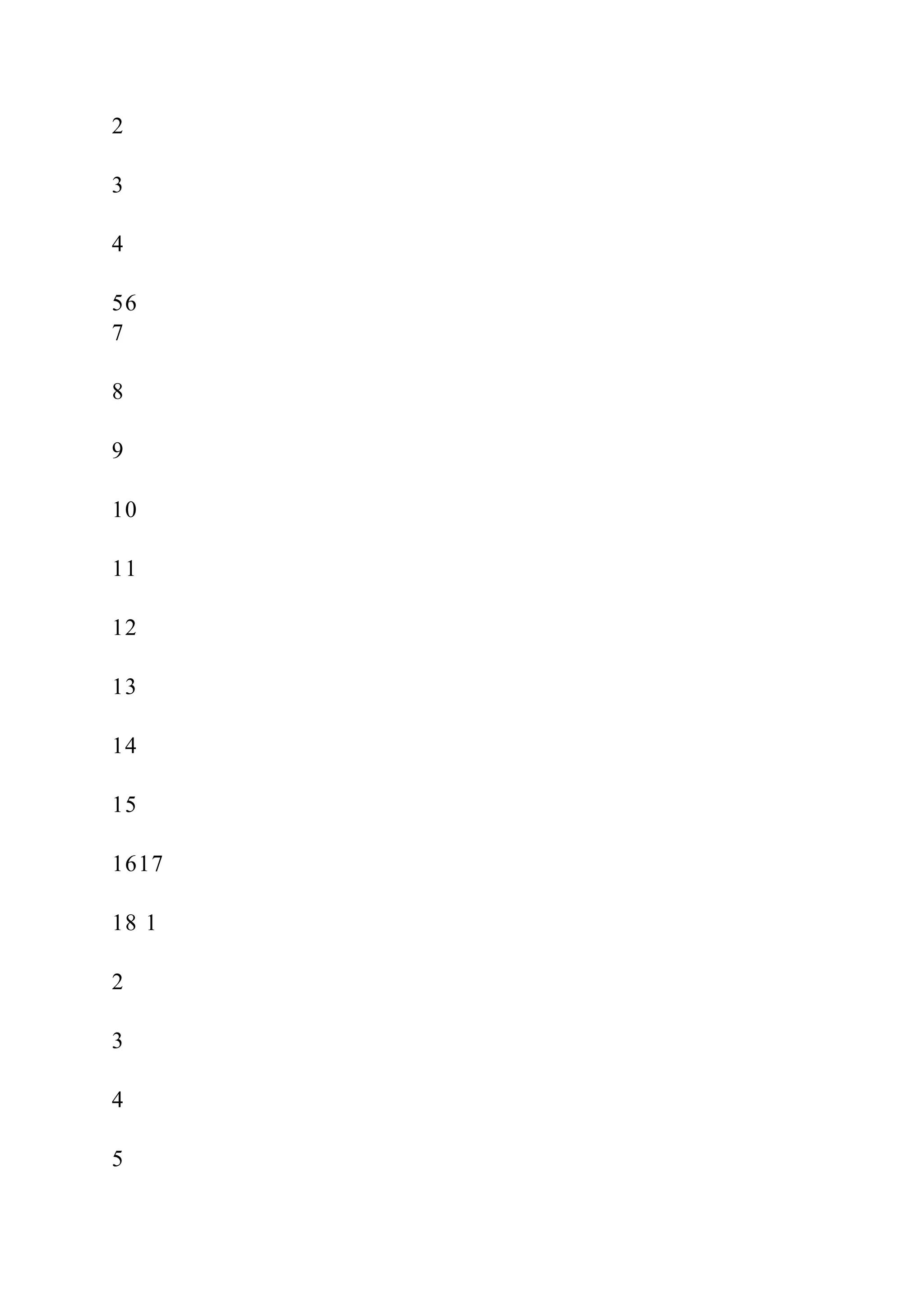
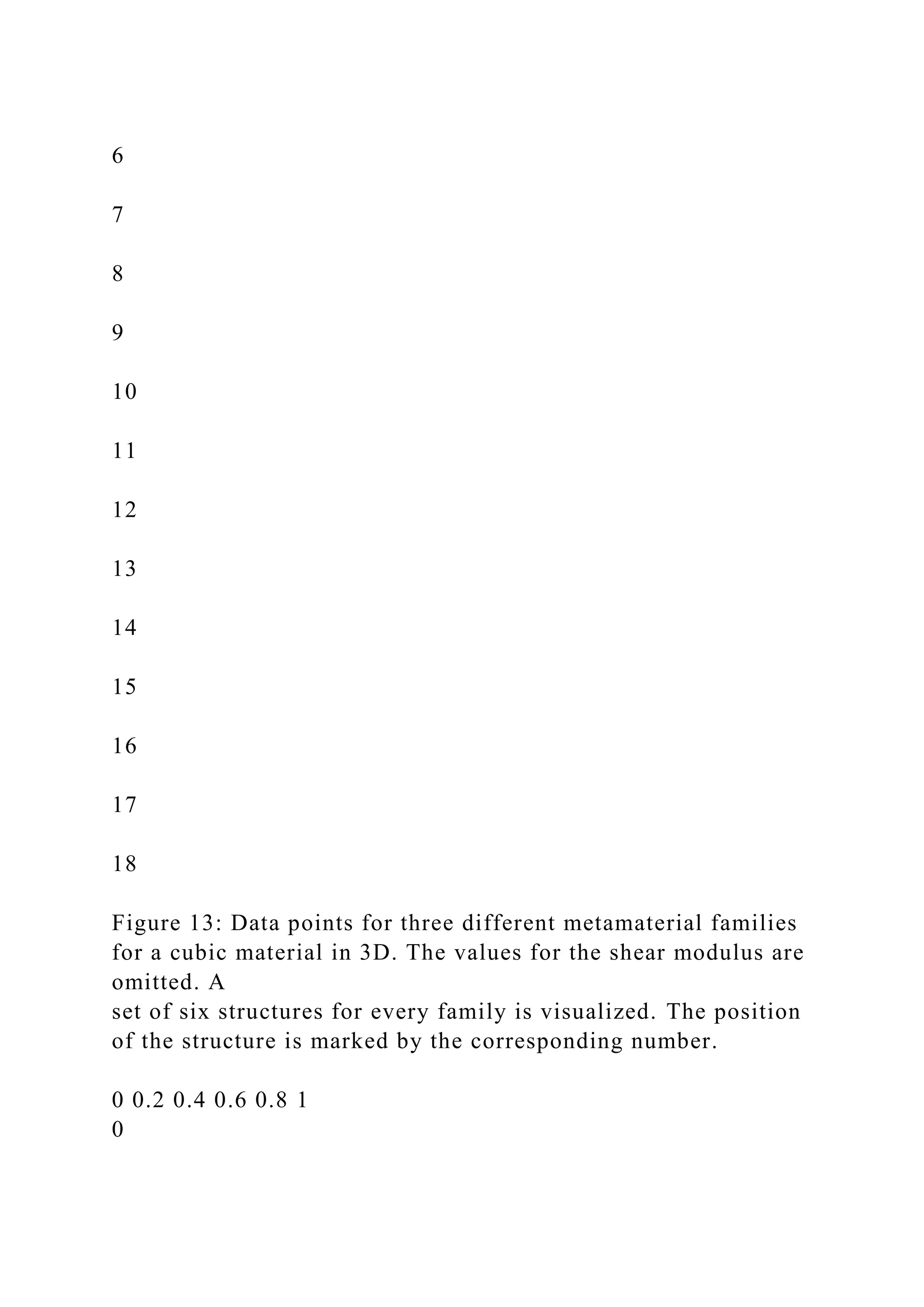
The microstructures in our database describe metamaterials with
certain properties; each gives a point sample of the mapping
from
material parameters to microstructures. Figure 13, 10, and 12 il-
lustrate data points for various metamaterial families. To
generate
a structure for an arbitrary given set of parameters, we
interpolate
between points of a family, forming a weighted average over a
set
of microstructures with similar elastic properties. We first com-
pute weights based on the inverse distance between the input
pa-
rameters and the parameters of the metamaterial space samples,
us-
ing the Wendland function with compact support [Nealen 2004].
We chose the parameter of the Wendland function such that the
weights vanish beyond a given interpolation radius, which is set
to 0.1 in normalized coordinates, or the distance to the (M + 1)-
nearest neighbor (M being the number of material parameters),
whichever is larger. Before we interpolate, we apply the
transfor-
mation f(x) = sgn(x) log(|x|+ δ) to transform the distance fields
to log space, and add a small constant δ = 10−3 to keep values
near
the surface. In practice, we found that interpolation in log space
re-
duces artifacts due to topology changes, e.g., holes appearing or
disappearing. Given the weights and transformed distance
fields,
we then compute the interpolated structure by linearly
interpolating
the transformed distance fields. Figure 7 illustrates the
interpolation
process.

6.3 Generating Metamaterial Families
Our metamaterial space consists of several, potentially
overlapping,
independent metamaterial families. We start the construction of
a
metamaterial family from a single microstructure, which we
either
model by hand based on existing examples from the literature,
or
obtain from our microstructure optimization (Sec. 5). We then
add
dilated and eroded versions of this initial microstructure to
achieve
a large initial sampling of the metamaterial space with good
inter-
polation properties. The dilation and erosion is performed
directly
on the distance field of the structure.
The metamaterial family construction then continues to do two
things: (i) Generate new candidates by evolving existing
structures,
which allows us to refine regions that are already covered by
sam-
ples, but with insufficient sampling density, and (ii) generate
new
candidates by optimizing for new microstructures outside of this
space. We proceed by alternating between these two stages until
136:7

both stages do not generate new microstructures.
Evolving Existing Microstructures The first stage is a heuris-
tic search based on the existing samples in the metamaterial
family.
For the refinement, we create the Delaunay triangulation of all
pa-
rameter points, and collect all the simplex centers. For every
cen-
ter, we check how well the parameters of the interpolated
structure
match the desired parameters, and add the interpolated structure
to
the metamaterial space if the deviation from the desired
parameters
is too large. For our experiments, we used a threshold of 0.1. In
3D, we additionally try to expand the metamaterial family in
this
stage. For this, we first compute the convex hull of all
parameter
samples. For every vertex on the convex hull, we then compute
an
offset point along the normal, which we use as the goal parame-
ters for a microstructure optimization. However, instead of
running
the optimization, we only compute the gradient of the objective
and
use it to change 2% of the activations in a discretized version of
the
current sample, which we then add to the metamaterial family.
Optimizing for New Microstructures The second stage is based
on the microstructure optimization introduced in Sec. 5. For the
re-

finement, we again compute the Delaunay triangulation and
check
how well the interpolation works at the simplex centers. If it is
insufficient, we run a microstructure optimization for the
parame-
ters at the simplex center with an initial guess computed from
the
weighted combination of all samples in the neighborhood of the
simplex center. Additionally, we introduce a similarity
regulariza-
tion, explained in more detail in the next paragraph. For the ex-
pansion, we again use the convex hull of all parameter samples
and
generate new parameters points by sampling the convex hull and
offsetting the points along the normal. For each of these points,
a
microstructure optimization is run, constructing the initial guess
in
the same way as for the refinement and using the same
additional
regularization.
For any new microstructure optimization that is run for a given
set
of parameters, the result should be similar to the existing struc-
ture to improve the interpolation. To lead the optimization into
the desired direction, an additional regularization is added to
the
optimization. This regularization penalizes the amount of
change
between a new structure and the structure of the N neighbors in
parameter space closest to the goal parameters. To allow for
small
changes, this penalty uses an exponential function:
Rsim =

N∑
i=1
w
i
sime
(
1
m
∑m
j=1
|αj−α
i
j
|
∆αi
)2
, (15)
where wisim = (N(1 + di))
−1 is the weight for neighbor i with
distance di to the desired parameters, αij is its j-th activation
and
∆αi = 0.1 + 2di is a threshold for the maximal desirable differ-
ence to this neighbor. Additionally, the initial activations for
the
optimization are set to a weighted average of the neighbors,
after a
smoothness step is applied. This reduces the risk of ending up

in a
local minimum.
7 Structure Synthesis
Using the microstructure optimization and parameter space sam-
pling methods, we can define several families of related
structures
that together span the feasible range of bulk material parameters
(Figure 10). Synthesizing a homogeneous material volume at
this
stage becomes trivial: We select a family that covers the desired
material behavior, compute the corresponding microstructure of
the cell by interpolation as described in Sec. 6.2, and then fill
the
Figure 8: The first 5 microstructures generated for a parameter
space without similarity regularization (top) and with similarity
regularization (bottom), starting from an initial structure (left).
volume by repeating this cell. Note that by construction this cell
is tileable. However, approximating spatially varying materials
is
more challenging.
Simply synthesizing microstructures for cells independently at
each
point in the model could lead to a mismatching boundary when
multiple different cells are tiled, as illustrated in Figure 9. Such
boundary mismatches will change the behavior of the cell,
which
was assumed to be in an infinite tiling of identical structures
when
its coarsened material parameters were computed. Therefore,
both
the geometry as well as the force profiles occurring at the

bound-
aries under deformation need to be taken into account. We
propose
a strategy that takes advantage of the multiple candidate
structures
for each cell provided by the overlapping families in our
metamate-
rial space. To compute an optimal selection from these
candidates,
we propose to minimize boundary dissimilarity between each
pair
of neighboring structures.
For a set of cells with desired parameters p1, . . . ,pk and
informa-
tion about the connectivity between cells, we interpolate one
struc-
ture for each cell from each of the l families, resulting in
structures
Si,1, . . . ,Si,l for every parameter sample pi. Finding the
optimal
choice of structures can then be formulated as a labeling
problem:
assign a structure to each cell to minimize a given cost function.
We propose a cost function that combines two types of costs.
The
labeling cost TLi,j = e
di,j describes how well a given structure Si,j
matches the desired parameters, and is based on the distance di,j
between pi and the material parameters of the structure as com-
puted by Numerical Coarsening.
The second cost TD(i,j),(r,s) = e
g(i,j),(r,s) is based on the dissimilar-

ity g(i,j),(r,s) of the boundaries of two neighboring structures
Si,j
and Sr,s. In most cases, it is sufficient to use the percentage of
the
boundary on which the two structures agree about the presence
or
absence of material. But since the problem of matching
boundaries
is linked to force discrepancies along the boundary during
defor-
mation, this dissimilarity can be improved by also considering
the
forces acting across the boundary. For this, we impose a unit
strain
Figure 9: Three potential configurations of two neighboring
cells.
Left: The individual structures closely match the desired
parame-
ters, but the boundaries are incompatible. Middle: Opposite
case.
Right: Our optimization computes a trade-off between the two
ex-
tremes.
0 0.2 0.4 0.6 0.8 1
0

0.1
0.2
0.3
0.4
0.5
0.6
0.7
0.8
0.9
1
Relative Young’s modulus [−]
Po
is
so
n
’s
ra
ti
o
[−
]

Figure 10: Data points for five different metamaterial families
for a
cubic material in 2D. The values for the shear modulus are
omitted.
on the boundary of each cell, such that they are stretched
perpen-
dicular to the boundary between the two cells. We then integrate
the
force magnitude as well as the force difference magnitude over
the
boundary, and set the dissimilarity g(i,j),(r,s) to the ratio of
force
difference magnitude to mean force magnitude. We compare the
two approaches to compute the boundary dissimilarity in Sec.
8.2.
Finding the globally optimal solution to this optimization
problem
is NP-hard. However, efficient algorithms exist that can find an
approximate solution. We employ an iterative method using
mes-
sage passing based on the alternating direction method of
multipli-
ers (ADMM) as described in Derbinsky et al. [2013].
For the resulting structures, the distance fields can then be com-
bined. To improve connectivity between cells, the smoothing
pass
is performed on the combined distance field instead of each cell
in-
dividually. The final structure is reconstructed from the
combined
distance field using marching cubes.

Connectivity Our synthesis method does not guarantee connec-
tivity. While we did not encounter cases of disconnected cells in
our
result, they can be detected easily and fixed by introducing
addi-
tional connections between disconnected structures, at the
expense
of the accuracy of the approximated elastic properties.
8 Results
8.1 Metamaterial Space Construction
We tested our method on three different material classes. In 2D,
we
generated metamaterial spaces for cubic materials (3
parameters)
and orthotropic materials (4 parameters), using a resolution of
402
voxels for the microstructure optimization. Due to the
inherently
anisotropic nature of square and cubic microstructures, we
found
that a cubic material space is better suited even for cases where
one is only interested in the Young’s modulus and Poisson’s
ratio
defining an isotropic material.
Figure 10 shows the Young’s modulus and Poisson’s ratio of
multi-
ple metamaterial families for a cubic material, and Figure 11
shows
the individual families as well as a subset of their structures.
While
a single family may span a wide range of parameters, this

example
shows that combining multiple families can significantly expand
this range. Figure 12 shows the orthotropic metamaterial
families,
projected into four different combinations of the parameter
axes.
We also used our method to compute a metamaterial space for
cubic
0 0.2 0.4 0.6 0.8 1
0
0.1
0.2
0.3
0.4
0.5
0.6
0.7
0.8
0.9
1
Po

is
so
n
’s
ra
ti
o
[−
]
0 0.2 0.4 0.6 0.8 1
0
0.1
0.2
0.3
0.4
0.5
0.6
0.7
0.8
0.9
1

Po
is
so
n
’s
ra
ti
o
[−
]
0 0.2 0.4 0.6 0.8 1
0
0.1
0.2
0.3
0.4
0.5
0.6
0.7
0.8

0.9
1
Po
is
so
n
’s
ra
ti
o
[−
]
0 0.2 0.4 0.6 0.8 1
0
0.1
0.2
0.3
0.4
0.5
0.6

0.7
0.8
0.9
1
Po
is
so
n
’s
ra
ti
o
[−
]
0 0.2 0.4 0.6 0.8 1
0
0.1
0.2
0.3
0.4

0.5
0.6
0.7
0.8
0.9
1
Po
is
so
n
’s
ra
ti
o
[−
]
Figure 11: The individual spaces from Figure 10, including a
visu-
alization of some of the structures.
materials in 3D (Figure 13), using a 163 voxels for the
microstruc-

ture optimization.
Timings For the microstructure optimization in 2D with a
resolu-
tion of 402, a single optimization step takes around 200 to 800
ms
to compute. The optimization usually converges in less than 500
iterations, resulting in a total computation time of several
minutes
per optimization. An optimization in 3D with a resolution of
163
runs with 8 to 30 seconds per iteration, and usually also
converges
in less than 500 iterations, for a total computation time of
around 2
hours per structure. Note that the metamaterial space
construction
is a pre-process that is only run once to build the database, and
it
can be easily parallelized.
For the structure synthesis, we tested the runtime of the
optimiza-
tion by combining three metamaterial spaces for different
numbers
of cells. For 400 cells, the optimization takes about 0.5 seconds,
for
2500 cells about 2 seconds and for 10000 cells on the order of
40
seconds. Synthesizing the distance fields and running the
optimiza-
tion took less than 10 seconds in all of our examples.
8.2 Validation

Our method relies on the ability to compute the material
behavior
of a microstructure from its design. To validate the results
obtained
by Numerical Coarsening, we tested several of our structures in
a
tensile test, and compared the results to our prediction. Since
we
are dealing with linear elasticity, the Numerical Coarsening and
the
optimization itself are independent of the Young’s modulus of
the
base material. The result can be adapted to any material with
the
same Poisson’s ratio by a simple scaling, meaning that the ratio
of the computed Young’s modulus of the microstructure and the
Young’s modulus of the base material is constant.
Our samples were fabricated by selective laser sintering of an
elas-
tic thermoplastic polyurethane (TPU 92A-1).
136:9
0 0.2 0.4 0.6 0.8 1
0
0.05
0.1

0.15
0.2
0.25
0.3
0.35
0.4
0.45
0.5
Po
is
so
n
’s
ra
ti
o
[−
]
1

2
3
4
56
7
8
9
10
11
12
13
14
15
1617
18 1
2
3
4
5

6
7
8
9
10
11
12
13
14
15
16
17
18
Figure 13: Data points for three different metamaterial families
for a cubic material in 3D. The values for the shear modulus are
omitted. A
set of six structures for every family is visualized. The position
of the structure is marked by the corresponding number.
0 0.2 0.4 0.6 0.8 1
0

0.1
0.2
0.3
0.4
0.5
0.6
0.7
0.8
0.9
1
Relative Young’s modulus E
x
[−]
R
e
la
ti
v
e
Y
o
u
n

g
’s
m
o
d
u
lu
s
E
y
[
−
]
0 0.2 0.4 0.6 0.8 1
0
0.1
0.2
0.3
0.4
0.5
0.6
0.7
0.8

0.9
1
Relative shear modulus [−]
R
e
la
ti
v
e
Y
o
u
n
g
’s
m
o
d
u
lu
s
E
y
[
−
]

0 0.2 0.4 0.6 0.8 1
−2
−1.5
−1
−0.5
0
0.5
1
1.5
Relative Young’s modulus E
x
[−]
P
o
is
s
o
n
’s
r
a
ti

o
ν
y
x
[
−
]
0 0.2 0.4 0.6 0.8 1
−2
−1.5
−1
−0.5
0
0.5
1
1.5
Relative shear modulus [−]
P
o
is
s
o

n
’s
r
a
ti
o
ν
y
x
[
−
]
Figure 12: Data points for four different metamaterial families
for
an orthotropic material in 2D. We show the relative Young’s
moduli
Ex and Ey the x-direction and y-direction, the relative shear
mod-
ulus and the Poisson’s ratio νyx that describes the contraction in
x-direction for an extension applied to the y-direction.
Figure 14: The
test setup.
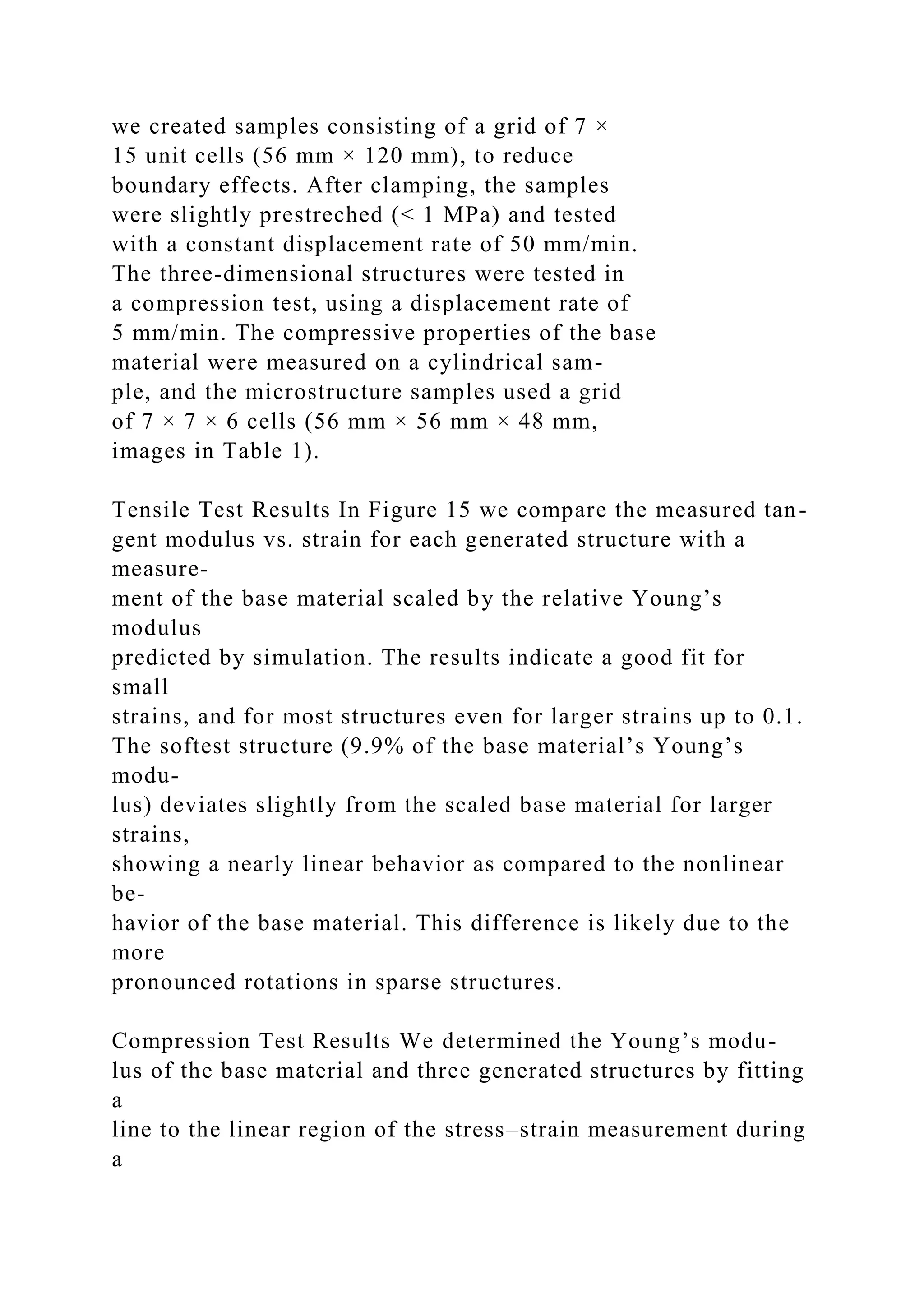
Test Setup and Method We used an Instron
E3000 frame with a 5 kN load cell for the ma-
terial test. For the 2D structures, we performed
tensile tests using a 10 cm pneumatic grip (Fig-
ure 14). We fist characterized the base mate-
rial using dog-bone shaped structures. To mea-
sure the tensile strength of the microstructures,

we created samples consisting of a grid of 7 ×
15 unit cells (56 mm × 120 mm), to reduce
boundary effects. After clamping, the samples
were slightly prestreched (< 1 MPa) and tested
with a constant displacement rate of 50 mm/min.
The three-dimensional structures were tested in
a compression test, using a displacement rate of
5 mm/min. The compressive properties of the base
material were measured on a cylindrical sam-
ple, and the microstructure samples used a grid
of 7 × 7 × 6 cells (56 mm × 56 mm × 48 mm,
images in Table 1).
Tensile Test Results In Figure 15 we compare the measured tan-
gent modulus vs. strain for each generated structure with a
measure-
ment of the base material scaled by the relative Young’s
modulus
predicted by simulation. The results indicate a good fit for
small
strains, and for most structures even for larger strains up to 0.1.
The softest structure (9.9% of the base material’s Young’s
modu-
lus) deviates slightly from the scaled base material for larger
strains,
showing a nearly linear behavior as compared to the nonlinear
be-
havior of the base material. This difference is likely due to the
more
pronounced rotations in sparse structures.
Compression Test Results We determined the Young’s modu-
lus of the base material and three generated structures by fitting
a
line to the linear region of the stress–strain measurement during
a

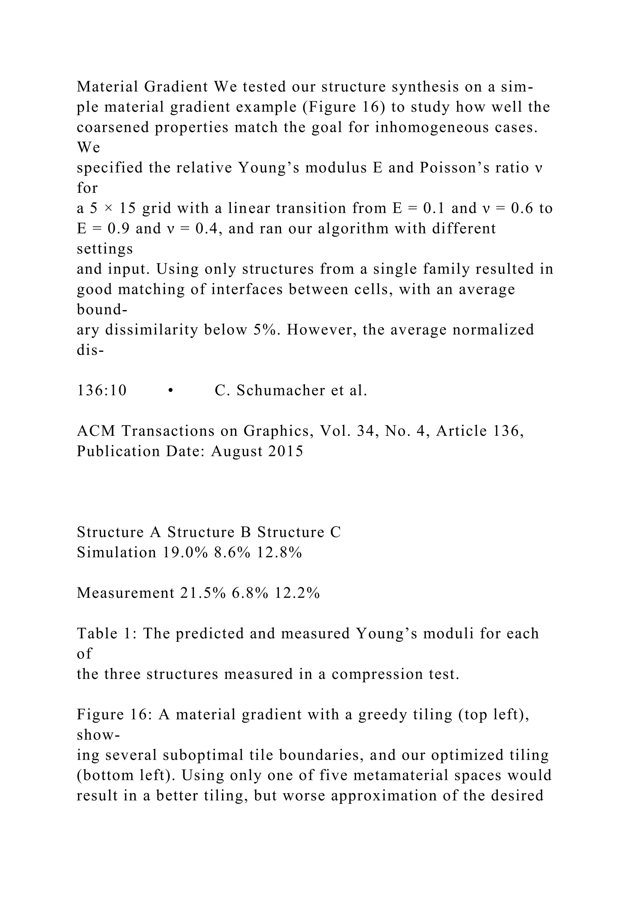
loading phase. Table 1 shows that the predicted and measured
rel-
ative Young’s modulus match reasonably well. The stress–strain
plots as well as the linear fits can be found in the supplemental
doc-
ument.
0 0.02 0.04 0.06 0.08 0.1
0
5
10
15
20
25
Engineering strain [−]
Ta
n
g
en
t
m
o
d
u
lu

s
[M
Pa
]
base material
structure 1
50.1% base material
structure 2
24.6% base material
structure 3
9.9% base material
0 0.02 0.04 0.06 0.08 0.1
0
5
10
15
20
25
Engineering strain [−]
Ta
n
g

en
t
m
o
d
u
lu
s
[M
Pa
]
base material
structure 4 (x−direction)
50.6% base material
structure 4 (y−direction)
20.5% base material
Figure 15: Tensile test results for a number of microstructures.
Top: Test results for synthesized microstructures with a
Young’s
modulus of 9.9%, 24.6% and 50.1% of the base material. The
scaled curve of the base material is shown for reference.
Bottom:
Test results for interpolated microstructures with orthotropic
ma-
terial behavior. The computed Young’s moduli were 20.5% and
50.6% of the base material’s Young’s modulus.

Material Gradient We tested our structure synthesis on a sim-
ple material gradient example (Figure 16) to study how well the
coarsened properties match the goal for inhomogeneous cases.
We
specified the relative Young’s modulus E and Poisson’s ratio ν
for
a 5 × 15 grid with a linear transition from E = 0.1 and ν = 0.6 to
E = 0.9 and ν = 0.4, and ran our algorithm with different
settings
and input. Using only structures from a single family resulted in
good matching of interfaces between cells, with an average
bound-
ary dissimilarity below 5%. However, the average normalized
dis-
Structure A Structure B Structure C
Simulation 19.0% 8.6% 12.8%
Measurement 21.5% 6.8% 12.2%
Table 1: The predicted and measured Young’s moduli for each
of
the three structures measured in a compression test.
Figure 16: A material gradient with a greedy tiling (top left),
show-
ing several suboptimal tile boundaries, and our optimized tiling
(bottom left). Using only one of five metamaterial spaces would
result in a better tiling, but worse approximation of the desired

ma-
terial parameters (right).
tances between the simulated parameters of the generated
structures
and the desired parameters were large, with values of 0.203,
0.075,
0.177, 0.228, and 0.104 for the five metamaterial families we
used
for this test. By using these metamaterial families to get a set of
can-
didate structures, we can greedily choose the best structure for
each
cell to achieve an average normalized distance of 0.051.
However,
there is no guarantee that these structures fit together, and
Figure 16
(orange) shows that the greedy synthesis generates poorly
fitting
transitions, with an average boundary dissimilarity of 15.3%.
Us-
ing the method described in Sec. 7, we can optimize for
parameter
approximation and boundary similarity at the same time. While
the
approximation of the desired parameters for the individual cells
is
slightly worse than for the greedy solution, with an average
normal-
ized distance of 0.065, the boundary dissimilarity in the
resulting
structure (Figure 16 (green)) was significantly better (4.2%).
Boundary Forces We presented two different approaches to rep-
resent the boundary dissimilarity during the synthesis stage.
Fig-

ure 17 shows a situation in which simply comparing the geome-
try of the boundary performs worse than comparing the
boundary
forces under unit strain. We used numerical coarsening to deter-
mine the material parameters of these structures, as well as the
pa-
rameters of a uniform mesh where each region is assigned the
coars-
ened material parameters of the corresponding cells in the
structure.
If only the geometries of the boundaries are compared, the
distance
between the actual parameters of the structure and the predicted
pa-
rameters is 0.0266, while the error is only 0.0137 if the
boundary
forces are used to predict the dissimilarity of the cell
boundaries.
Figure 17: Two gradients computed for the same goal parame-
ters, using geometry (left) and boundary forces (right) to
estimate
the boundary dissimilarity during synthesis. The actual material
parameters for the right structure deviate less from the predicted
parameters (error of 0.0266, left, and 0.0137, right).
Effects of Heterogeneity We explored our method’s perfor-
mance for strongly heterogeneous goal parameters with two dif-
ferent tests, looking at the influence of the spatial frequency
and
amplitude of parameter changes on the prediction error. On a
grid
of 12 × 12 cells, we synthesized structure patterns using
sinusoids
to define the goal Young’s moduli. We tested frequencies from
a

single period across the grid to 6 periods (i.e. a checkerboard),
and
amplitudes of parameter change ranging up to 45%, with a mean
of 50% of the base material (so stiffnesses range from 5% to
95%
at the highest amplitude). We computed the difference between
the
homogenized material parameters of the synthesized structure
and
the homogenized material parameters of a uniform mesh with
local
material parameters set to the goals for the individual cells.
Even
though the assumption of infinite homogenous tilings is
violated,
Figure 18 shows that for such heterogeneous tilings, the
prediction
error is below 0.05 even for very drastic parameter changes, and
only above that in extreme cases where the change from
maximal
to minimal parameters happens in a span of less than two cells,
or
the amplitude is larger than 0.35.
1 2 3 4 5 6
0
0.05
0.1
0.15
0.2
0.25

0.3
0.35
0.4
Frequency multiplier
Pr
ed
ic
ti
o
n
e
rr
o
r
0.1 0.2 0.3 0.4
0
0.01
0.02
0.03
0.04
0.05

0.06
0.07
0.08
0.09
0.1
Parameter amplitude
Pr
ed
ic
ti
o
n
e
rr
o
r
Figure 18: The influence of a heterogeneous tiling on the
approx-
imation error, based on a 12 × 12 grid with a sinusoidal distri-
bution of Young’s moduli. The colors of the plot match the
meta-
material families shown in Figure 10. We also show the spatial
distribution of the Young’s moduli at the top of the plots
(blue=soft,

orange=stiff). Top: The error plotted for varying numbers of
peri-
ods for the parameter distribution, with an amplitude of 45%
(solid
line) and 20% (dashed line). A frequency multiplier of 6 corre-
sponds to a checkerboard distribution. Bottom: The error plotted
for different amplitudes, with a frequency multiplier of 3 (solid
line)
and 2 (dashed line).
136:11
Figure 19: The optimized structure for the gripper (left), the
gen-
erated model (middle). The fabricated result (right) can be used
to
grab and lift small objects.
8.3 Application Examples
Gripper Inspired by the field of soft robotics, we designed a
sim-
ple gripper that can be actuated by air pressure (Figure 19). The
gripper consists of two hollow tubes 16cm in length, printed
with
a soft material. The tubes are designed as a 2D structure with a
stiff material on one half and an anisotropic material on the
other
half that is soft along the tube and stiff along the
circumferential

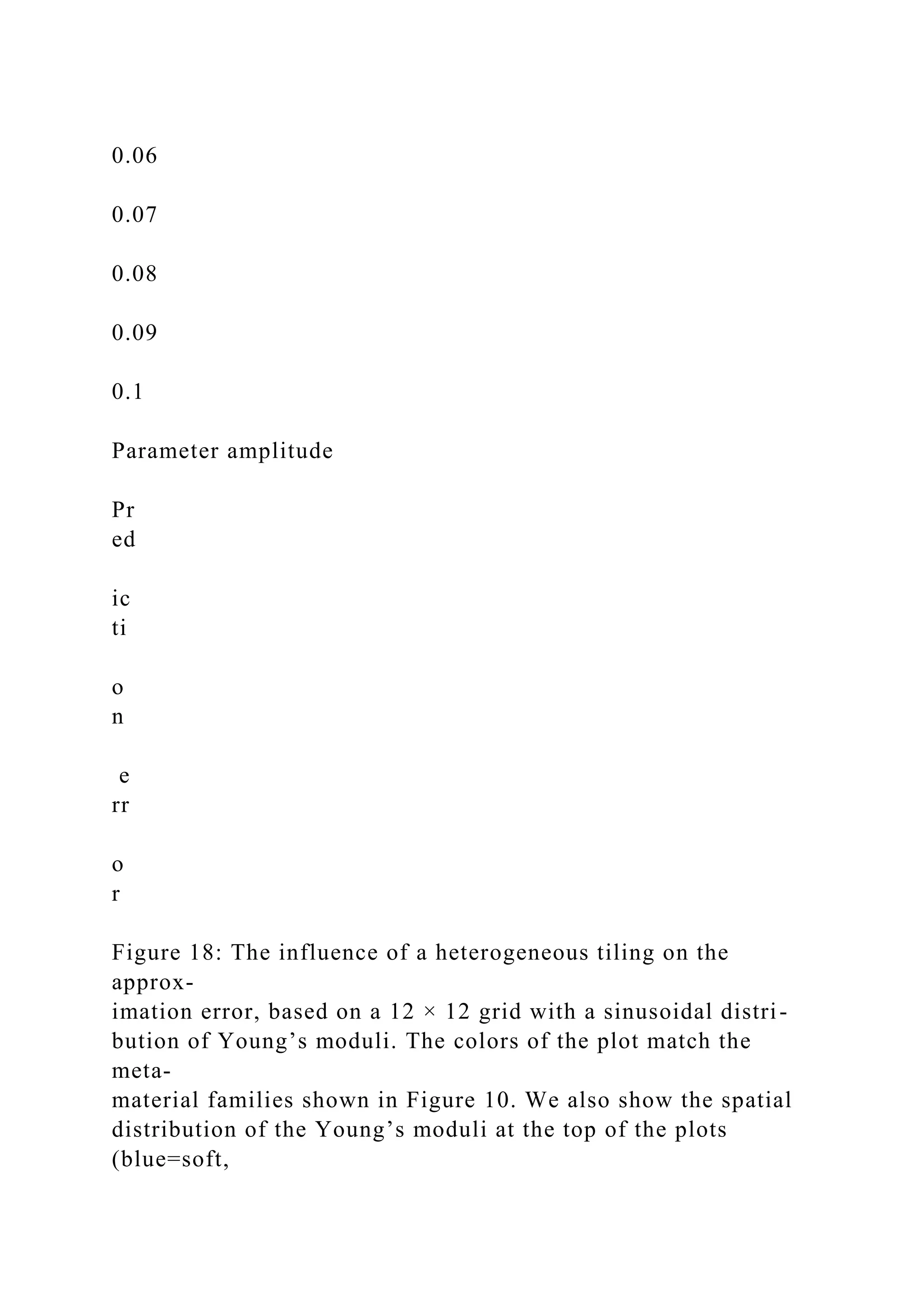
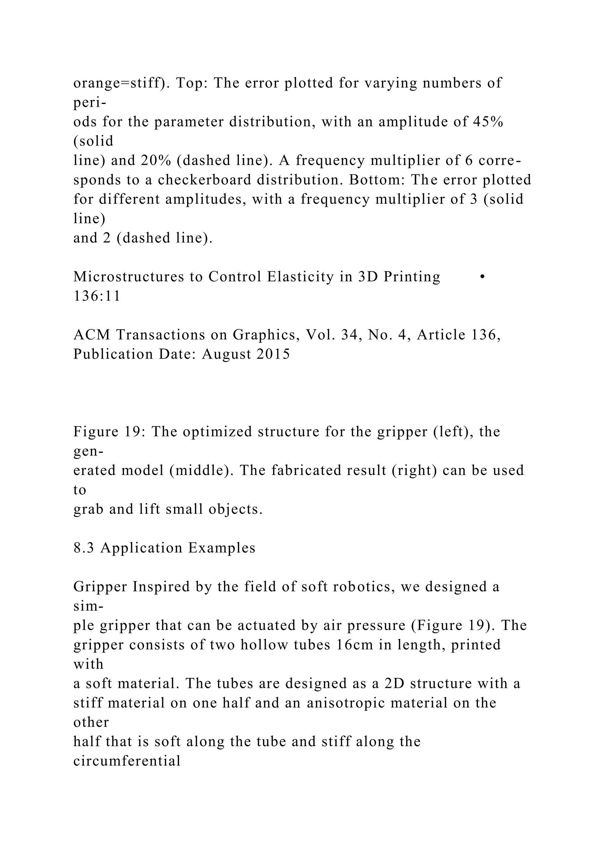
direction. A balloon is inserted into each tube, and increasing
the
pressure inside the balloons causes the tubes to bend due to the
dif-
ference in stiffness. At the same time, the anisotropy of the
struc-
ture prevents large changes in diameter. While this is only a
very
simple actuator, we believe that our method will be an
important
step towards a design tool for printable soft robots.
Bunny, Teddy, and Armadillo For the three-dimensional case,
we tested our pipeline on two models (Bunny, 13 cm high;
Teddy,
15 cm) with spatially varying Young’s moduli, created with an
in-
teractive material design tool [Xu et al. 2015]. The models were
subdivided into cells with 8 mm side length, and the Young’s
mod-
uli averaged for each cell. The metamaterial space used to
populate
these cells contained a single family of 21 microstructures. For
synthesis, we chose the nearest neighbor in the database for
each
Young’s modulus. To keep the shape of the models, the
individual
voxels of each structure were set to void if they lay outside of
the
model. While this might lead to disconnected components in the
re-
construction, these can easily be removed. We created a third
model
(Armadillo, 32 cm high) by manually painting the desired
Young’s
modulus into a volumetric mesh, which was then used as an

input
to our method, using cells with 8 mm side length. We chose the
parameter distribution such that the joints and the belly of the
Ar-
madillo are soft, while all other parts of the model are stiff. The
structure of the cells were computed and tiled using our
synthesis
algorithm with the metamaterial space shown in Figure 13. The
fab-
ricated model can be easily actuated, as shown in the
accompanying
video, even though the base material is quite stiff.
9 Conclusion
We have presented a complete framework for automatically con-
verting a given object with specified elastic material parameters
into a fabricable representation that resembles the desired
elastic
deformation behavior. Our approach efficiently generates small-
scale structures that obtain their elastic bulk properties from the
shape and arrangement of the structures, significantly
expanding the
gamut of materials reproducible by 3D printers. Although our
ap-
proach relies on an extensive pre-computation phase for
generating
families of related structures that can be interpolated to
smoothly
vary the material properties, this only needs to be done once.
We
plan to publicly release our database of structures. To create an
ob-
ject with spatially varying elastic properties, our approach tiles
the
object’s interior with microstructures drawn from the database,

us-
ing an efficient algorithm to select compatible structures for
neigh-
boring cells.
Limitations and Future Work Our method targets output devices
that can 3D print at high resolution, and that allow easy removal
of support material. In practice, we found selective laser
sintering
the most convenient process because the part is surrounded by
un-
sintered powder and therefore does not require support
structures.
Removal of the unsintered powder from the structures can be
easily
achieved with compressed air. Other technologies, such as poly-
jet or fused deposition modeling, allow printing overhangs
without
support structures only up to a certain angle. For future work,
an
interesting avenue could be incorporating these constraints into
the
optimization of material structures, spanning a space of
metamate-
rials that are printable without support on these machines.
In our current work we focused on linear elasticity and small
strain
deformations. In the future, we plan to extend our approach to
non-
linear material behavior, also incorporating interesting
structures
with buckling behavior. Another highly interesting avenue
would
be the detection of localized stresses and considering points of

fail-
ure in the material structure during the optimization, improving
the
robustness of the material.
Finally, in our current implementation we do not explicitly treat
the boundaries of the object, and obtain the boundary by simply
intersecting the geometry of the structures with the shape of the
object. An interesting next step would be wrapping the object
with
a surface for aesthetic reasons, but also taking the surface’s
effect
on the deformation into account.
Acknowledgments
We would like to thank the reviewers for their insightful
comments,
and Jernej Barbič for providing models and material parameter
dis-
tributions for the Bunny and Teddy examples. We also greatly
ap-
preciated the help of Moritz Bächer, Jonathan Yedidia, Mélina
Sk-
ouras, and Oliver Wang. The Bunny and Armadillo models are
part of the Stanford Computer Graphics Laboratory’s 3D
Scanning
Repository.
References
ATTARD, D., AND GRIMA, J. N. 2012. A three-dimensional
ro-
tating rigid units network exhibiting negative poisson’s ratios.
physica status solidi (b) 249, 7, 1330–1338.

BABAEE, S., SHIM, J., WEAVER, J. C., PATEL, N., AND
BERTOLDI, K. 2013. 3d soft metamaterials with negative pois-
son’s ratio. Advanced Materials 25, 5044–5049.
BECKER, M., AND TESCHNER, M. 2007. Robust and efficient
estimation of elasticity parameters using the linear finite
element
method. In Proceedings of the Conference on Simulation and
Visualization (SimVis), 15–28.
BICKEL, B., BÄCHER, M., OTADUY, M. A., LEE, H. R.,
PFIS-
TER, H., GROSS, M., AND MATUSIK, W. 2010. Design and
fabrication of materials with desired deformation behavior.
ACM
Trans. Graph. (Proc. SIGGRAPH) 29, 3.
BYRD, R. H., LU, P., NOCEDAL, J., AND ZHU, C. 1995. A
limited memory algorithm for bound constrained optimization.
SIAM J. Sci. Comput. 16, 1190–1208.
CHEN, D., LEVIN, D. I. W., DIDYK, P., SITTHI-AMORN, P.,
AND MATUSIK, W. 2013. Spec2Fab: A reducer-tuner model
for translating specifications to 3D prints. ACM Trans. Graph.
(Proc. SIGGRAPH) 32, 4.
CIORANESCU, D., AND DONATO, P. 2000. Introduction to
ho-

mogenization.
COELHO, P., FERNANDES, P., GUEDES, J., AND
RODRIGUES, H.
2008. A hierarchical model for concurrent material and topol-
ogy optimisation of three-dimensional structures. Structural and
Multidisciplinary Optimization 35, 2, 107–115.
DERBINSKY, N., BENTO, J., ELSER, V., AND YEDIDIA, J.
S.
2013. An improved three-weight message-passing algorithm.
arXiv:1305.1961.
DONG, Y., WANG, J., PELLACINI, F., TONG, X., AND GUO,
B.
2010. Fabricating spatially-varying subsurface scattering. ACM
Trans. Graph. (Proc. SIGGRAPH) 29, 4.
HAŠAN, M., FUCHS, M., MATUSIK, W., PFISTER, H., AND
RUSINKIEWICZ, S. 2010. Physical reproduction of materials
with specified subsurface scattering. ACM Trans. Graph. (Proc.
SIGGRAPH) 29, 4.
HASHIN, Z., AND SHTRIKMAN, S. 1963. A variational
approach
to the theory of the elastic behaviour of multiphase materials.
Journal of the Mechanics and Physics of Solids 11, 2, 127–140.
HILLER, J., AND LIPSON, H. 2012. Automatic design and
man-
ufacture of soft robots. Robotics, IEEE Transactions on 28, 2,
457–466.
HUANG, X., RADMAN, A., AND XIE, Y. 2011. Topological
design of microstructures of cellular materials for maximum
bulk or shear modulus. Computational Materials Science 50,

6, 1861–1870.
HUGHES, T., MARMIER, A., AND EVANS, K. 2010. Auxetic
frameworks inspired by cubic crystals. International Journal of
Solids and Structures 47, 11.
KHAREVYCH, L., MULLEN, P., OWHADI, H., AND
DESBRUN,
M. 2009. Numerical coarsening of inhomogeneous elastic ma-
terials. ACM Trans. Graph. (Proc. SIGGRAPH) 28, 51.
LAKES, R. 1987. Foam structures with a negative poisson’s
ratio.
Science 235, 4792, 1038–1040.
LAN, Y., DONG, Y., PELLACINI, F., AND TONG, X. 2013.
Bi-
scale appearance fabrication. ACM Trans. Graph. (Proc. SIG-
GRAPH) 32, 4.
LEE, J.-H., SINGER, J. P., AND THOMAS, E. L. 2012. Micro-
/nanostructured mechanical metamaterials. Advanced Materials
24, 36, 4782–4810.
MICHEL, J., MOULINEC, H., AND SUQUET, P. 1999.
Effective
properties of composite materials with periodic microstructure:
a computational approach. Computer methods in applied me-
chanics and engineering 172, 1, 109–143.
NEALEN, A., MÜLLER, M., KEISER, R., BOXERMAN, E.,
AND
CARLSON, M. 2006. Physically based deformable models in
computer graphics. Computer Graphics Forum 25, 4, 809–836.
NEALEN, A. 2004. An as-short-as-possible introduction to the

least
squares, weighted least squares and moving least squares meth-
ods for scattered data approximation and interpolation. Tech.
rep., TU Darsmstadt.
NESME, M., KRY, P. G., JEŘÁBKOVÁ, L., AND FAURE, F.
2009.
Preserving topology and elasticity for embedded deformable
models. ACM Trans. Graph. (Proc. SIGGRAPH) 28, 3.
REINER, T., CARR, N., MECH, R., STAVA, O.,
DACHSBACHER,
C., AND MILLER, G. 2014. Dual-color mixing for fused de-
position modeling printers. Computer Graphics Forum (EURO-
GRAPHICS 2014 Proceedings) 33, 2.
RODRIGUES, H., GUEDES, J., AND BENDSOE, M. 2002.
Hier-
archical optimization of material and structure. Structural and
Multidisciplinary Optimization 24, 1, 1–10.
ROUILLER, O., BICKEL, B., KAUTZ, J., MATUSIK, W., AND
ALEXA, M. 2013. 3d-printing spatially varying brdfs. Com-
puter Graphics and Applications, IEEE 33, 6.
SIFAKIS, E., AND BARBIC, J. 2012. Fem simulation of 3d de-
formable solids: a practitioner’s guide to theory, discretization
and model reduction. In ACM SIGGRAPH 2012 Courses, 20.
SIGMUND, O., AND PETERSSON, J. 1998. Numerical
instabilities
in topology optimization: a survey on procedures dealing with
checkerboards, mesh-dependencies and local minima. Structural
optimization 16, 1, 68–75.
SIGMUND, O. 2009. Systematic design of metamaterials by

topol-
ogy optimization. In IUTAM Symposium on Modelling
Nanoma-
terials and Nanosystems, Springer, 151–159.
SKOURAS, M., THOMASZEWSKI, B., COROS, S., BICKEL,
B.,
AND GROSS, M. 2013. Computational design of actuated de-
formable characters. ACM Trans. Graph. (Proc. SIGGRAPH)
32, 4.
SMIT, R., BREKELMANS, W., AND MEIJER, H. 1998.
Prediction
of the mechanical behavior of nonlinear heterogeneous systems
by multi-level finite element modeling. Computer Methods in
Applied Mechanics and Engineering 155, 1, 181–192.
STAVA, O., VANEK, J., BENES, B., CARR, N., AND MĚCH,
R.
2012. Stress relief: improving structural strength of 3d printable
objects. ACM Trans. Graph. (Proc. SIGGRAPH) 31, 4.
VIDIMČE, K., WANG, S.-P., RAGAN-KELLEY, J., AND MA-
TUSIK, W. 2013. Openfab: A programmable pipeline for multi-
material fabrication. ACM Trans. Graph. (Proc. SIGGRAPH)
32.
WANG, W., WANG, T. Y., YANG, Z., LIU, L., TONG, X.,
TONG,
W., DENG, J., CHEN, F., AND LIU, X. 2013. Cost-effective
printing of 3d objects with skin-frame structures. ACM Trans.
Graph. (Proc. SIGGRAPH Asia) 32, 6.
WEYRICH, T., PEERS, P., MATUSIK, W., AND
RUSINKIEWICZ,
S. 2009. Fabricating microgeometry for custom surface re-

flectance. ACM Trans. Graph. (Proc. SIGGRAPH) 28, 3.
XU, H., LI, Y., CHEN, Y., AND BARBIČ, J. 2015. Interactive
ma-
terial design using model reduction. ACM Trans. Graph. (TOG)
34, 2.
ZHOU, S., AND LI, Q. 2008. Design of graded two-phase mi-
crostructures for tailored elasticity gradients. Journal of Materi-
als Science 43, 15, 5157–5167.
ZHOU, Q., PANETTA, J., AND ZORIN, D. 2013. Worst-case
struc-
tural analysis. ACM Trans. Graph. (Proc. SIGGRAPH) 32, 4.
136:13
Assignment: Expansion Recommendation
Introduction
This portfolio work project will allow you to review
information and risks associated with an investment to expand
an organization. As this information will be shared broadly
across the organization, you will have a choice in your final
deliverable audience and will organize your deliverable to meet
the needs of that audience.
Scenario
ZXY Company is a food product company. ZXY is considering
expanding to two new products and a second production facility.
The food products are staples with steady demands. The
proposed expansion will require an investment of $7,000,000

for equipment with an assumed ten-year life, after which all
equipment and other assets can be sold for an estimated
$1,000,000. They will be renting the facility. ZXY requires a 12
percent return on investments. You have been asked to
recommend whether or not to make the investment.
Your Role
You are an accounting manager. Your boss has asked you to
review and provide a recommendation on the expansion based
on information that has been provided.
Requirements
In preparing and supporting your recommendation to either
make the investment or not, include the following items as part
of your analysis:
· Analysis of financial information.
· Identification of risks associated with the investment.
Consider:
· How risky the project appears.
· How far off your estimates of revenues and expenses can be
before your decision would change.
· The difference if the company were to use a straight line
versus a MACRS depreciation.
· Recommendation for a course of action.
· Explanation of criteria supporting your recommendation.
Financial Information
As part of your analysis you might find that additional
information from marketing, accounting, or finance would be
useful in making an informed and well-supported
recommendation. In a real workplace setting you would have the
ability to ask for that information. However, for the purposes of
this assignment, you can make assumptions about the values of
that data or ratios in support of your recommendation.
Accounting worked with the marketing group to create the ZXY
Company Financial Statements spreadsheet provided in the
Resources for the new products business and the new facility.
Notes about the financial information:
· The expense line labeled SQF FDA Mandates refers to the

costs of complying with Food and Drug Administration
requirements.
· Depreciation expense is calculated using 7-year life modified
accelerated cost recovery system (MACRS).
Deliverable Format
Depending on the audience you choose to address, use one of
the following options:
· Report for a mid-management audience. Prepare a 3–4 page
report detailing your recommendation and the information you
used to make your recommendation.
· Presentation for top leadership. Prepare a presentation of at
least 12 slides detailing your recommendation and the
information you used to make your recommendation. You may
use your choice of presentation software. Include notes with
additional details.
Related company standards for either format:
· The recommendation report is a professional document and
should therefore follow the corresponding MBA Academic and
Professional Document Guidelines, including single-spaced
paragraphs.
· In addition to the report or presentation, include:
· Title (slide or page).
· References (slide or page).
· Appendix with supporting materials.
· At least two APA-formatted references.
Paper Analysis Project
Introduction
The project requires you to read a computer-graphics-related
paper and write a 5-page

(1.5 spacing) analysis of it.
The 5-page Paper You Submit Must At Least Cover
1. What is the general theme of the paper you read? What does
the title mean?
Wjat are they trying to do? Why are they trying to do it? (I.e.,
what problem are
they trying to solve?)
2. Who are the authors? Where are they from? What positions
do they hold? Can
you find out something about their backgrounds?
3. What did the authors do?
4. What conclusions did the paper draw?
5. What insights did you get from the paper that you didn't
already know?
6. Did you see any flaws or short-sightedness in the paper's
methods or
conclusions? (It's OK if you didn't.)
7. If you were these researchers, what would you do next in this
line of research?
You can, and should, copy-and-paste a key image or two from
the paper to help
explain what it is about. Do not make these images huge in an
effort to consume what
should have been writing space!

Spacing needs to be 1.5
There needs to be a cover page, and, no, that doesn't count as
one of the 5 pages...

ACM Reference FormatSchumacher, C., Bickel, B., Rys, J., Mar.docx

Recommended

Recommended

More Related Content

Similar to ACM Reference FormatSchumacher, C., Bickel, B., Rys, J., Mar.docx

Similar to ACM Reference FormatSchumacher, C., Bickel, B., Rys, J., Mar.docx (20)

More from daniahendric

More from daniahendric (20)

Recently uploaded

Recently uploaded (20)

ACM Reference FormatSchumacher, C., Bickel, B., Rys, J., Mar.docx