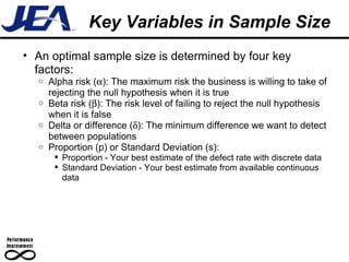
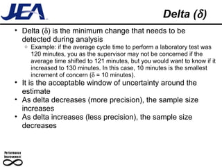
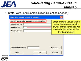
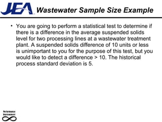
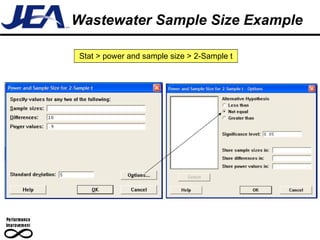
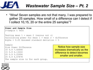
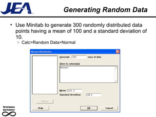
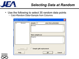
This document discusses key factors in determining sample size for statistical analysis: alpha risk, beta risk, delta or difference, and proportion or standard deviation. It provides examples of calculating sample size using Minitab for a wastewater treatment example comparing two processing lines, and selecting a random sample from a larger data set. The homework asks the reader to calculate sample sizes needed to determine if an invoice defect rate is different than 10% if the observed rates are 12%, 15%, 20%, or 25%.

1. Sample Size Determination Deliverable 10A

2. Analyze Module Roadmap Define 1D – Define VOC, VOB, and CTQ’s 2D – Define Project Boundaries 3D – Quantify Project Value 4D – Develop Project Mgmt. Plan Measure 5M – Document Process 6M – Prioritize List of X’s 7M – Create Data Collection Plan 8M – Validate Measurement System 9M – Establish Baseline Process Cap. Analyze 10A – Determine Critical X’s Improve 12I – Prioritized List of Solutions 13I – Pilot Best Solution Control 14C – Create Control System 15C – Finalize Project Documentation Green 11G – Identify Root Cause Relationships Queue 1 Queue 2

3. Objectives – Sample Size Upon completion of this module, the student should be able to: List and define the variables which contribute to determining the correct sample size. Calculate the appropriate sample size for a defined set of variables

4. Key Variables in Sample Size An optimal sample size is determined by four key factors: Alpha risk (  ): The maximum risk the business is willing to take of rejecting the null hypothesis when it is true Beta risk (  ): The risk level of failing to reject the null hypothesis when it is false Delta or difference (  ): The minimum difference we want to detect between populations Proportion (p) or Standard Deviation (s): Proportion - Your best estimate of the defect rate with discrete data Standard Deviation - Your best estimate from available continuous data

5. Alpha Risk (  ) Alpha risk is decided by the Black Belt Our choice of  will determine when to reject the null hypothesis Typical  values for general business applications are between 0.05 and 0.10. As the cost of incorrect conclusions go up, you may choose to lower  . e.g. Pharmaceutical companies have tremendous risk to consumer health issues and often use an  of 0.01 The  value should depend on practical considerations such as financial or safety risk, or risk to the customer “ Significance” is defined as 1- 

6. Beta Risk (  ) Beta risk can be selected by the Black Belt, but we don‘t control it the same way we do  risk. The best we can do is adjust sample size so that  is no greater than a specified value. When a beta error (  ) occurs, we have missed detecting a difference (good or bad). Power is defined as (1 -  ). It represents the probablitily that we can detect an important effect in the process Typical values of power in experiments are between 0.80 to 0.90 We will use 0.90 for most work at JEA

7. Delta (  ) Delta (  ) is the minimum change that needs to be detected during analysis Example: if the average cycle time to perform a laboratory test was 120 minutes, you as the supervisor may not be concerned if the average time shifted to 121 minutes, but you would want to know if it increased to 130 minutes. In this case, 10 minutes is the smallest increment of concern (  = 10 minutes). It is the acceptable window of uncertainty around the estimate As delta decreases (more precision), the sample size increases As delta increases (less precision), the sample size decreases

8. Signal to Noise Ratio If you consider  and  , the ratio of the two is much like a signal-to-noise ratio If the “signal” is large relative to the noise, we can “hear” the signal Sample size will increase dramatically as the  ratio drops Low  High  

9. Minitab Versus Excel Minitab uses an “infinite population” approach Minitab calculators assume the population is relatively infinite Relatively infinite means the population is at least ten times larger than the sample used Predicts a “safe” sample size (larger than a finite population approach) Excel calculators are able to use a “finite population” approach They have a “finite population correction factor” Adjusts the sample size to account for when we are sampling a significant portion of the population

10. Calculating Sample Size in Minitab Stat>Power and Sample Size>{Select as needed} Enter multiple values with a space between values for any/all of these (Minitab will calculate the value for the third parameter)

11. Wastewater Sample Size Example You are going to perform a statistical test to determine if there is a difference in the average suspended solids level for two processing lines at a wastewater treatment plant. A suspended solids difference of 10 units or less is unimportant to you for the purpose of this test, but you would like to detect a difference > 10. The historical process standard deviation is 5.

12. Wastewater Sample Size Example Stat > power and sample size > 2-Sample t

13. Minitab Output Power and Sample Size 2-Sample t Test Testing mean 1 = mean 2 (versus not =) Calculating power for mean 1 = mean 2 + difference Alpha = 0.05 Assumed standard deviation = 5 Sample Target Difference Size Power Actual Power 10 7 0.9 0.929070 The sample size is for each group.

14. Wastewater Sample Size – Pt. 2 “ Wow! Seven samples are not that many. I was prepared to gather 25 samples. How small of a difference can I detect if I collect 10,15, 20 or the entire 25 samples”? Power and Sample Size 2-Sample t Test Testing mean 1 = mean 2 (versus not =) Calculating power for mean 1 = mean 2 + difference Alpha = 0.05 Assumed standard deviation = 5 Sample Size Power Difference 10 0.9 7.66846 15 0.9 6.13222 20 0.9 5.25996 25 0.9 4.67878 The sample size is for each group. Notice how sample size increases dramatically as the difference to detect becomes smaller and smaller.

15. Class Exercise Recalculate the sample size for the previous problem using a 1%  and a 0.80 power. 10 min

16. Homework - Back to Pat’s Invoice Problem Our old friend Pat is starting to wonder about the validity of a great number of past decisions. In this case, Pat now realizes that the past practice of guessing at the number of invoices to inspect (as was done in previous modules) wasn’t the most reliable. How many data points will Pat need to inspect to rule in/out that the process does not have a 10% defect rate if the samples inspected had a 12%, 15%, 20%, or 25% defect rate?

17. Selecting Data for the Stat Test Now that we know how many data points to include in the statistical test, we need to identify which samples should be placed in the test. Assume you have several hundred data points collected over time, but the sample size calculation showed you need only 35 for the statistical test. How do we pick the appropriate 35? The 35 “best” or “worst” will certainly skew our conclusions 35 from the center of the data will not show the appropriate variability Let’s have Minitab do it for us!

18. Generating Random Data Use Minitab to generate 300 randomly distributed data points having a mean of 100 and a standard deviation of 10. Calc>Random Data>Normal

19. Selecting Data at Random Use the following to select 35 random data points Calc>Random Data>Sample from Columns

20. Randomly Selected Data This procedure works equally well with text or numerical values (a wonderful way to select the sequence for Black Belts to present their projects in class).

21. Learning Check – Sample Size Upon completion of this module, the student should be able to: List and define the variables which contribute to determining the correct sample size. Calculate the appropriate sample size for a defined set of variables