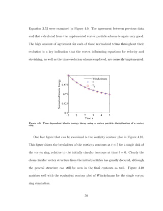
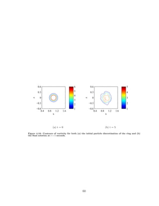
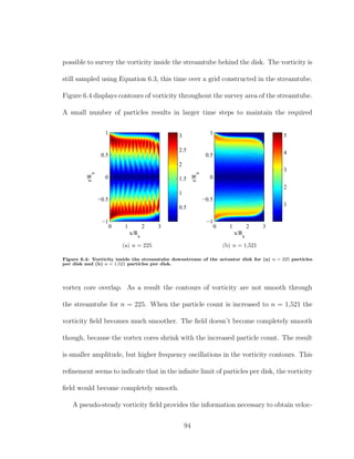
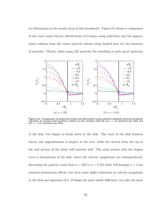
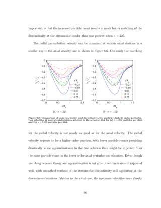
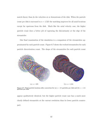
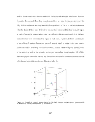
This thesis presents a new method for modeling propeller-airframe interaction using a three dimensional vortex particle-panel code. The method combines a flexible aerodynamic panel code with a pseudo-steady slipstream model that discretizes rotational effects onto vortex particle point elements. Verification and validation studies were conducted to ensure an accurate model. The method provides a useful tool for conceptual aircraft design by allowing rapid testing of configurations without requiring volume grids. The thesis describes the development of the new method and presents simulations of several configurations to demonstrate its capabilities.
![vorticity field can be written as
ωN
σ (x, t) =
p
[αp
(t) ζσ (x − xp
(t)) + (αp
(t) · (Gσ (x − xp
(t))))] . (3.22)
Winckelmans rewrites Equation 3.22 as
ωN
σ (x, t) =
p
ζσ (x − xp
(t)) −
qσ (x − xp
(t))
|x − xp (t) |3
αp
(t) +
3
qσ (x − xp
(t))
|x − xp (t) |3
− ζσ (x − xp
(t))
((x − xp
(t)) · αp
(t))
|x − xp (t) |2
(x − xp
(t)) . (3.23)
It has been shown that the regularized particle method converges to the solution
of the respective formulation of the momentum equation selected, either classical,
transpose, or mixed, for some finite time T.29–31,33
The proofs show that as the number
of particles increases and the corresponding vortex core sizes decrease, the error norm
decreases to zero.
3.4 Viscous Diffusion
As mentioned, one of the major strengths of the vortex particle method is its
ability to account for viscous diffusion. This feature is extremely valuable because
it has been demonstrated to help maintain a nearly divergence-free particle vorticity
field necessary for a valid solution.34
The transpose scheme applied to the vorticity-
velocity form of the momentum equation with viscous effects is written
∂ω
∂t
+ · (ωu) = ω · T
u + ν 2
ω, (3.24)
30](https://image.slidesharecdn.com/d538c7a1-7d13-4b63-a79e-b29df7bce89c-150718042220-lva1-app6892/85/A-Three-Dimensional-Vortex-Particle-Panel-Code-For-Modeling-Prope-50-320.jpg)
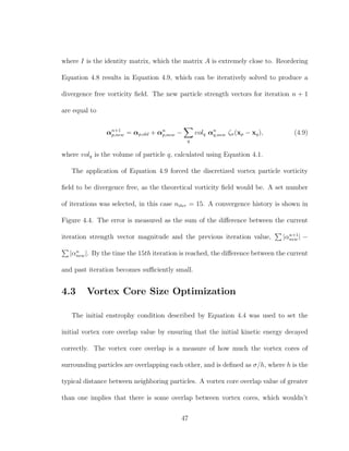
![free vorticity field, ω(xp
(0), 0).
Mathematically, new particle strength vectors are desired that cause the particle
vorticity field and exact vorticity to be equal,
ω(xp
(0), 0) = ωσ(xp
(0), 0). (4.5)
The particle discretized vorticity field of the left hand side, for which the particle
strength vector is the unknown, is defined in Equation 3.12. The exact vorticity field
is defined as ω(xp
(0), 0) = αp
(0)/volp
. Plugging these definitions into Equation 4.5
gives
q
αq
new(0) ζσ(xp
− xq
(0)) =
αp
old(0)
volp
. (4.6)
Thus, the new particle strength vectors, αnew, were a function of the old strength
vectors, αold, the particle locations, xp and xq, and the particle volumes, vol, as well
as the regularization function, ζσ. By defining the matrix [A] = [volpζσ(xp − xq)]
Equation 4.6 can be rewritten as
[A]αnew = αold. (4.7)
For high particle counts in the study it quickly becomes impossible to invert the
[A] matrix, and to circumvent this problem an iterative scheme has been employed,
relying on the fact that the initial strengths, αold, are good guesses for the final
strength values, αnew, that make the vortex particle vorticity field divergence free.
The iterative scheme suggested by Beale40
recasts Equation 4.6 as
(A − I)αnew + αnew = αold, (4.8)
46](https://image.slidesharecdn.com/d538c7a1-7d13-4b63-a79e-b29df7bce89c-150718042220-lva1-app6892/85/A-Three-Dimensional-Vortex-Particle-Panel-Code-For-Modeling-Prope-66-320.jpg)
![5.1.1 Theory
The most fundamental building block of the Conway method, and the Hough and
Ordway method, is the vortex ring, and the influence it exerts. The streamfunction
and velocity field of a vortex ring can be expressed in terms of elliptic integrals as
ψ(r, z) =
Γ(ar)1/2
2π
Q1/2(ω1), (5.1)
Vr(r, z) =
Γ(z − z ) k1 [(2 − k2
1)E(k1) − 2(1 − k2
1)K(k1)]
8π(1 − k2
1)(a r3)1/2
(5.2)
Vz(r, z) =
Γ k1[k2
1(a2
− r2
− z2
)E(k1) + 4 r a(1 − k2
1)K(k1)]
16π(1 − k2
1)(r a)3/2
(5.3)
where
k1 ≡
4 a r
(a + r)2 + (z − z )2
1/2
, (5.4)
ω1 ≡ 1 +
(a − r)2
+ (z − z )2
2ar
, (5.5)
and Q(x) is a Legendre function of the second kind, E(k) is a complete elliptic integral
of the second kind, K(k) is a complete elliptic integral of the first kind, Γ(ω) is the
Gamma function, z is the z location of the vortex ring, and a is the radius of the ring.
These equations represent an alternative to the singularity that traditionally appears
when considering flow induced by a vortex ring as the ring itself is approached.
Much as vortex particle theory relies on the Biot-Savart law to describe the induced
velocity field, actuator disk theory uses Biot-Savart to find instantaneous velocities in
the field. In this case though, the velocity information is time averaged, and based on
the time averaged vorticity distribution, which is constructed of two vortex systems,
63](https://image.slidesharecdn.com/d538c7a1-7d13-4b63-a79e-b29df7bce89c-150718042220-lva1-app6892/85/A-Three-Dimensional-Vortex-Particle-Panel-Code-For-Modeling-Prope-83-320.jpg)
![total pressure change from one side of the disk to the other is
∆po = p+
o − p−
o = (p+
+ q+
) − (p−
+ q−
) = (p+
− p−
) = ∆p. (5.33)
Therefore, knowledge of the pressure change at the disk can provide information about
the total pressure change. Additionally, total pressure is constant along a streamline,
so the total pressure change at any point in the field can be determined by tracing a
streamline back to the disk and determining the total pressure change at the disk.
The ∆p term of the actuator disk is related to the loading and the thrust the disk
produces. As Lotstedt 7
states
∆p =
dT
2πrdr
. (5.34)
Additionally, we know from actuator disk theory that
dT = 2πρr Vz(r, ∞)(U∞ + Vz(r, ∞)) −
V 2
φ (r, ∞)
2
dr. (5.35)
Plugging Equation 5.35 into Equation 5.34 gives a relationship for ∆p in terms of the
velocity profile at downstream infinity
∆p = ρ Vz(r, ∞)(U∞ + Vz(r, ∞)) −
V 2
φ (r, ∞)
2
. (5.36)
Using the linearized actuator disk theory, where Vz(r, ∞) = 2Vz(r, 0), results in
∆p = ρ 2Vz(r, 0)(U∞ + Vz(r, 0)) −
V 2
φ (r, ∞)
2
. (5.37)
Finally, assuming a contra-rotating actuator disk with no swirl results in
∆p = 2ρ [Vz(r, 0)(U∞ + Vz(r, 0))] . (5.38)
79](https://image.slidesharecdn.com/d538c7a1-7d13-4b63-a79e-b29df7bce89c-150718042220-lva1-app6892/85/A-Three-Dimensional-Vortex-Particle-Panel-Code-For-Modeling-Prope-99-320.jpg)
![Thus, depending on the assumptions that are suitable to make, we have a relation-
ship that describes the pressure jump at the disk. It is convenient to change these
relationships to pressure coefficient jumps because it eliminates the requirement for a
density being specified. The pressure coefficient jump is simply equal to the pressure
jump divided by the freestream dynamic pressure,
∆Cp =
1
1
2
U2
∞
Vz(r, ∞)(U∞ + Vz(r, ∞)) −
V 2
φ (r, ∞)
2
. (5.39)
With the linearized actuator disk theory assumption we have
∆Cp =
1
1
2
U2
∞
2Vz(r, 0)(U∞ + Vz(r, 0)) −
V 2
φ (r, ∞)
2
. (5.40)
The contra-rotating actuator disk assumption yields
∆Cp =
2
1
2
U2
∞
[Vz(r, 0)(U∞ + Vz(r, 0))] . (5.41)
The most critical location requiring knowledge of the actuator disk pressure jump
is on the surface of the geometry, as this is where the most detailed experimental
information was measured via surface pressure taps. The pressure jump here was
easy to measure, with the first step being to use the specified velocity distribution at
the disk to determine the total velocity along the surface of the nacelle. This velocity
and the freestream velocity are the only terms required to find the pressure coefficient
jump via Equation 5.41. This method is valid because the surface of the nacelle is a
streamline passing through the disk root, and the pressure jump is constant along a
streamline from the disk to downstream infinity. It becomes much more difficult to
80](https://image.slidesharecdn.com/d538c7a1-7d13-4b63-a79e-b29df7bce89c-150718042220-lva1-app6892/85/A-Three-Dimensional-Vortex-Particle-Panel-Code-For-Modeling-Prope-100-320.jpg)
![simultaneously orthogonal to each other, and the third is normal to the panel. An
example of panel coordinates for an arbitrary panel are shown in 7.1.
−1.5
0
1.5 −1.5
0
1.5
−1.5
0
1.5
y
x
z
Figure 7.1: Panel coordinates on an arbitrary panel relative to global coordinates.
To convert any point whose global coordinates are known into panel coordinates,
it is first necessary to construct a transformation matrix, composed of the three
components of each of the three coordinate unit vectors.
T =
l1 l2 l3
m1 m2 m3
n1 n2 n3
. (7.1)
To obtain the point of interest in the panel coordinate frame the vector point of
interest location is multiplied by the transformation vector.
[x, y, z]panel = [x, y, z]globalT. (7.2)
Converting a local velocity vector into global coordinates follows the same procedure
118](https://image.slidesharecdn.com/d538c7a1-7d13-4b63-a79e-b29df7bce89c-150718042220-lva1-app6892/85/A-Three-Dimensional-Vortex-Particle-Panel-Code-For-Modeling-Prope-138-320.jpg)
![as the conversion of a vector position. The position vectors of Equation 7.2 are simply
replaced by the velocity vectors, [u, v, w]panel and [u, v, w]global.
The panel coordinate transformation becomes even more complex when converting
a velocity gradient calculated in local coordinates back to the global frame. The cal-
culated velocity gradient is the change in local velocity in each of the local coordinate
axes. This means the calculated gradient is
∂u
∂x
=
∂u
∂x
∂v
∂x
∂w
∂x
∂u
∂y
∂v
∂y
∂w
∂y
∂u
∂z
∂v
∂z
∂w
∂z
, (7.3)
where the prime indicates local coordinates, while the desired gradient information is
∂u
∂x
=
∂u
∂x
∂v
∂x
∂w
∂x
∂u
∂y
∂v
∂y
∂w
∂y
∂u
∂z
∂v
∂z
∂w
∂z
. (7.4)
A simple conversion like the one in Equation 7.2 won’t return the entire gradient
to global coordinates. Instead two consecutive conversions are necessary, as shown in
Equation 7.5.
u = [ u T]T
T (7.5)
The first transform of Equation 7.5 is applied as indicated in Equation 7.2, which
returns part of 7.3 to global coordinates, resulting in
∂u
∂x
=
∂u
∂x
∂v
∂x
∂w
∂x
∂u
∂y
∂v
∂y
∂w
∂y
∂u
∂z
∂v
∂z
∂w
∂z
T =
∂u
∂x
∂v
∂x
∂w
∂x
∂u
∂y
∂v
∂y
∂w
∂y
∂u
∂z
∂v
∂z
∂w
∂z
. (7.6)
The result is a matrix that describes the change in local velocity components with
change in global coordinates. Thus, a second transformation is required to return
the velocities to global coordinates as well. To do this, the rows of the matrix to
119](https://image.slidesharecdn.com/d538c7a1-7d13-4b63-a79e-b29df7bce89c-150718042220-lva1-app6892/85/A-Three-Dimensional-Vortex-Particle-Panel-Code-For-Modeling-Prope-139-320.jpg)
![−0.1 0 0.1 0.2 0.3 0.4 0.5 0.6 0.7 0.8
−0.1
−0.05
0
0.05
0.1
x
z
Figure 7.4: A 2D example of streamlines generated from the time stepping technique around a 3D
symmetric wing panel solution.
necessary because pressure coefficient data would only be known on the surface of the
paneled geometry at each panel collocation point. There was no guarantee that the
collocation points would fall at each of the experimental pressure port locations.
Wing Interpolation
An interpolation method was applied to the wing, where data was interpolated
in terms of i and j matrix indices instead of x, y, and z. The structured nature of
the paneling made interpolation in the surface feasible, and likely the best possible
solution in terms of elegance and accuracy. Interpolation in the i − j frame starts
with finding the [i, j] matrix indices that identify the collocation points bounding the
point where pressure coefficient data is desired. Once the bounding indices are known,
linear interpolation is carried out independently in the i and then j dimensions.
Nacelle Interpolation
Since the wind tunnel pressure taps fall in axial rings along the nacelle, with
multiple ports appearing at each single axial slice, the collocation point data was
131](https://image.slidesharecdn.com/d538c7a1-7d13-4b63-a79e-b29df7bce89c-150718042220-lva1-app6892/85/A-Three-Dimensional-Vortex-Particle-Panel-Code-For-Modeling-Prope-151-320.jpg)

![Bibliography
[1] Willis, D. J., An Unsteady, Accelerated, High Order Panel Method with Vortex
Particle Wakes, Ph.D. thesis, Massachusetts Institute of Technology, 2006.
[2] Colin, P., Moreux, V., and Barillier, A., “Numerical Study of Aerodynamic High
Speed Propeller Engine Integration on Transport Aircraft,” 20th Congress of the
International Council of the Aeronautical Sciences, International Council of the
Aeronautical Sciences, 1996, pp. 2366–2380.
[3] Winckelmans, G. S., Topics in Vortex Methods for Computation of Three- and
Two-Dimensional Incompressible Unsteady Flows, Doctor of philosophy, Califor-
nia Institute of Technology, Pasadena, California, February 1989.
[4] Morgenthal, G., Aerodynamic Analysis of Structures Using High-Resolution Vor-
tex Particle Methods, Doctor of philosophy, University of Cambridge, October
2002.
[5] Willis, D. J., “FastAero - a precorrected FFT - Fast Multipole Tree Steady
and Unsteady Potential Flow Solver,” Tech. rep., Massachusetts Institute of
Technology, 2005.
197](https://image.slidesharecdn.com/d538c7a1-7d13-4b63-a79e-b29df7bce89c-150718042220-lva1-app6892/85/A-Three-Dimensional-Vortex-Particle-Panel-Code-For-Modeling-Prope-217-320.jpg)
![[6] Opoku, D. G., Triantos, D. G., Nitzsche, F., and Voutsinas, S. G., “Rotor-
craft Aerodynamic and Aeroacoustic Modelling Using Vortex Particle Methods,”
ICAS Congress, 2002.
[7] Lotstedt, P., “Propeller Slip-Stream Model in Subsonic Linearized Potential
Flow,” Journal of Aircraft, Vol. 29, No. 6, November-December 1992, pp. 1098–
1105.
[8] E, Q., Yang, G., and Li, F., “Numerical Analysis of the Interference Effect of
Propeller Slipstream on Aircraft Flowfield,” Journal of Aircraft, Vol. 35, No. 1,
January-February 1998, pp. 84–90.
[9] Samuelsson, I., “Experimental Investigation of Low Speed Model Propeller
Slipstream Aerodynamic Characteristics Including Flow Field Surveys and Na-
celle/Wing Static Pressure Measurements,” Congress of the International Coun-
cil of the Aeronautical Sciences, Vol. 17, FFA, The Aeronautical Research Insti-
tute of Sweden, 1990, pp. 71–84.
[10] Shapiro, A., “Film Notes for Vorticity,” National Committee for Fluid Mechanics
Films, 1969.
[11] Williis, D. J., Peraire, J., and White, J. K., “A Combined pFFT-multipole Tree
Code, Unsteady Panel Method with Vortex Particle Wakes,” International Jour-
nal for Numerical Methods in Fluids, Vol. 00, 2000, pp. 1–6.
198](https://image.slidesharecdn.com/d538c7a1-7d13-4b63-a79e-b29df7bce89c-150718042220-lva1-app6892/85/A-Three-Dimensional-Vortex-Particle-Panel-Code-For-Modeling-Prope-218-320.jpg)
![[12] Winckelmans, G., Cocle, R., Dufresne, L., and Capart, R., “Vortex Methods
and their Application to Trailing Wake Vortex Simulation,” Comptes Rendus
Physique, Vol. 6, 2005, pp. 467–486.
[13] Chatelain, P., Curioni, A., Bergdorf, M., Rossinelli, D., Andreoni, W., and
Koumoutsakos, P., “Billion Vortex Particle Direct Numerical Simulations of
Aircraft Wakes,” Computer Methods in Applied Mechanics and Engineering,
Vol. 197, 2007, pp. 1296–1304.
[14] Opoku, D. G. and Nitzsche, F., “Acoustic Validation of a New Code Using Par-
ticle Wake Aerodynamics and Geometrically-Exact Beam Structural Dnyamics,”
29th European Rotorcraft Forum, 2003.
[15] Conway, J. T. and Su, J., “PMAL Flow Calculations for the Aurora Aircraft
Using Non-axisymmetric Propeller Actuator Disks,” Canadian Aeronautics and
Space Journal, Vol. 49, No. 1, March 2003, pp. 1–9.
[16] Strash, D. and Lednicer, D., “Analysis of propeller-induced aerodynamic effects,”
16th AIAA Applied Aerodynamics Conference, 1998.
[17] Dang, T., “Simulations of Propeller/Airframe Interference Effects Using an Euler
Corrrection Method,” Journal of Aircraft, Vol. 26, 1989, pp. 994–1001.
199](https://image.slidesharecdn.com/d538c7a1-7d13-4b63-a79e-b29df7bce89c-150718042220-lva1-app6892/85/A-Three-Dimensional-Vortex-Particle-Panel-Code-For-Modeling-Prope-219-320.jpg)
![[18] Kuijvenhoven, J., “Validation of Propeller Slipstream Calculations Using a
Multi-Block Euler Code,” AIAA 8th Applied Aerodynamic Conference, Applied
Aerodynamics, AIAA, AIAA, August 1990.
[19] Hess, J. and Valarezo, W., “Calculation of steady flow about propellers using a
surface panel method,” Journal of Propulsion and Power, Vol. 1, No. 6, January
1986, pp. 470–476.
[20] Rizk, M., “Propeller Slipstream/Wing Interaction in the Transonic Regime,”
Journal of Aircraft, Vol. 18, No. 3, March 1981, pp. 184–191.
[21] Whitfield, D. and Jameson, A., “Euler Equation Simulation of Propeller-Wing
Interaction in Transonic Flow,” Journal of Aircraft, Vol. 21, No. 11, November
1984, pp. 835–839.
[22] Samuelsson, I., “Low Speed Propeller Slipstream Aerodynamic Effects,” Tech.
rep., FFA, The Aeronautical Research Institute of Sweden, 1994.
[23] Samuelsson, I., “Low Speed Wind Tunnel Investigation of Propeller Slipstream
Aerodynamic Effects on Different Nacelle/Wing Combinations,” Congress of the
International Council of the Aeronautical Sciences, Vol. 16, Congress of the
International Council of the Aeronautical Sciences, August-September 1988, pp.
1749–1765.
200](https://image.slidesharecdn.com/d538c7a1-7d13-4b63-a79e-b29df7bce89c-150718042220-lva1-app6892/85/A-Three-Dimensional-Vortex-Particle-Panel-Code-For-Modeling-Prope-220-320.jpg)
![[24] Fratello, G., Favier, D., and Maresca, C., “Experimental and Numerical Study
of Propeller/Fixed Wing Interaction,” Journal of Aircraft, Vol. 28, No. 6, June
1991, pp. 365–373.
[25] Witkowski, D. P., Lee, A. K., and Sullivan, J. P., “Aerodynamic Interaction
Between Propellers and Wings,” Journal of Aircraft, Vol. 26, No. 9, September
1989, pp. 829–836.
[26] Stuermer, A., “Unsteady Euler and Navier-Stokes Simulations of Propellers with
Unstructured DLR TAU-Code,” New Results in Numerical and experimental
Fluid Mechanics V , Vol. 92, 2006, pp. 144–151.
[27] Cho, J. and Williams, M. H., “Propeller-Wing Interaction Using a Frequency
Domain Panel Method,” Journal of Aircraft, Vol. 27, No. 3, March 1990, pp. 196–
203.
[28] Rehbach, C., “Numerical Calculation of Three-Dimensional Unsteady Flows with
Vortex Sheets,” Aerospace Sciences Meeting, 1978.
[29] Beale, J. T. and Majda, A., “Vortex Methods I: Convergence in Three Dimen-
sions,” Mathematics of Computation, Vol. 39, No. 159, July 1982, pp. 1–27.
[30] Beale, J. T. and Majda, A., “Vortex Method II: Higher Order Accuracy in Two
and Three Dimensions,” Mathematics of Computation, Vol. 39, No. 159, July
1982, pp. 29–52.
201](https://image.slidesharecdn.com/d538c7a1-7d13-4b63-a79e-b29df7bce89c-150718042220-lva1-app6892/85/A-Three-Dimensional-Vortex-Particle-Panel-Code-For-Modeling-Prope-221-320.jpg)
![[31] Beale, J. T., “A Convergent 3-D Vortex Method With Grid-Free Stretching,”
Mathematics of Computation, Vol. 46, No. 174, April 1986, pp. 401–424.
[32] Saffman, P. and Meiron, D., “Difficulties with Three-Dimensional Weak Solutions
for Inviscid Incompressible Flow,” Phys. Fluids, Vol. 29, No. 8, August 1986,
pp. 2373–2375.
[33] Cottet, G.-H., “A new approach for the analysis of Vortex Methods in two and
three dimensions,” Ann. Inst. Henri Poincare, Vol. 5, No. 3, 1988, pp. 227–285.
[34] Winckelmans, G. and Leonard, A., “Contributions to Vortex Particle Meth-
ods for the Computation of Three-Dimensional Incompressible Unsteady Flows,”
Journal of Computational Physics, Vol. 109, 1993, pp. 247–273.
[35] Degond, P. and Mas-Gallic, S., “The Weighted Particle Method for Convection-
Diffusion Equations Part 1:The Case of an Isotropic Viscosity,” Mathematics of
Computation, Vol. 53, No. 188, October 1989, pp. 485–507.
[36] Degond, P. and Mas-Gallic, S., “The Weighted Particle Method for Convection-
Diffusion Equations Part 2: The Anisotropic Case,” Mathematics of Computa-
tion, Vol. 53, No. 188, October 1989, pp. 509–525.
[37] Choquin, J. and Huberson, S., “Particle Simulation of Viscous Flow,” Computers
and Fluids, Vol. 17, No. 2, 1989, pp. 397–410.
202](https://image.slidesharecdn.com/d538c7a1-7d13-4b63-a79e-b29df7bce89c-150718042220-lva1-app6892/85/A-Three-Dimensional-Vortex-Particle-Panel-Code-For-Modeling-Prope-222-320.jpg)
![[38] Benfatto, G., Picco, P., and Pulvirenti, M., “On the Invariant Measures for the
Two-Dimensional Euler Flow,” Journal of Statistical Physics, Vol. 46, No. 3/4,
1987, pp. 729–742.
[39] Cottet, G.-H. and Koumoutsakos, P. D., Vortex Methods: Theory and Practice,
Cambridge University Press, 2000.
[40] Beale, J., “On The Accuracy of Vortex Methods at Large Times,” Tech. rep.,
Institute for Mathematics and its Applications, 1987.
[41] Williamson, J., “Low-Storage Runge-Kutta Schemes,” Journal of Computational
Physics, Vol. 35, 1980, pp. 48–56.
[42] Carpenter, M. H. and Kennedy, C. A., “Fourth-Order 2N-Storage Runge-Kutta
Schemes,” NASA Technical Memorandum 109112, NASA, June 1994.
[43] Carpenter, M. H. and Kennedy, C. A., “Third-Order 2N-Storage Runge-Kutta
Schemes with Error Control,” NASA Technical Memorandum 109111, NASA,
June 1994.
[44] Wilson, R. V., Demuren, A. O., and Carpenter, M., “Higher-Order Compact
Schemes for Numerical Simulation of Incompressible Flows,” NASA ICASE Re-
port 98-13, NASA, February 1998.
203](https://image.slidesharecdn.com/d538c7a1-7d13-4b63-a79e-b29df7bce89c-150718042220-lva1-app6892/85/A-Three-Dimensional-Vortex-Particle-Panel-Code-For-Modeling-Prope-223-320.jpg)
![[45] Kennedy, C. A., Carpenter, M. H., and Lewis, R. M., “Low-Storage, Explicit
Runge-Kutta Schemes for the Compressible Navier-Stokes Equations,” NASA
CR ICASE 99-22, NASA, 1999.
[46] Calvo, M., Franco, J., and Randez, L., “A New Minimum Storage Runge-
Kutta Scheme for Computational Acoustics,” Journal of Computational Physics,
Vol. 201, 2004, pp. 1–12.
[47] Butcher, J. C., The Numerical Analysis of Ordinary Differential Equations:
Runge-Kutta and General Linear Methods, Wiley Interscience, 1987.
[48] Conway, J. T., “Analytical Solutions for the Actuator Disk with Variable Radial
Distribution of Load,” Journal of Fluid Mechanics, Vol. 297, 1995, pp. 327–355.
[49] Conway, J. T., “Exact Actuator Disk Solutions For Non-uniform Heavy Load-
ing and Slipstream Contraction,” Journal of Fluid Mechanics, Vol. 365, 1998,
pp. 235–267.
[50] Conway, J. T., “Prediction of the Performance of Heavily Loaded Propellers
with Slipstream Contraction,” Canadian Aeronautics and Space Journal, Vol. 44,
No. 3, September 1998, pp. 169–174.
[51] Hough, G. and Ordway, D., “The Generalized Actuator Disk,” Developments in
Theoertical and Applied Mechanics, Vol. 2, 1965, pp. 317–336.
[52] Conway, J., “Personal Correspondence with Rob McDonald,” 9/4/2009.
204](https://image.slidesharecdn.com/d538c7a1-7d13-4b63-a79e-b29df7bce89c-150718042220-lva1-app6892/85/A-Three-Dimensional-Vortex-Particle-Panel-Code-For-Modeling-Prope-224-320.jpg)
![[53] VonMises, R., Theory of Flight, McGraw-Hill, 1945.
[54] Lamb, S. H., Hydrodynamics, Dover Publications, 1945.
[55] Strain, J., “2D Vortex Methods and Singular Quadrature Rules,” Journal of
Computational Physics, Vol. 124, No. 49, 1996, pp. 131–145.
[56] Leonard, A., Koumoutsakos, P., and Winckelmans, G., “Vortex Methods for
Three-Dimensional Separated Flows,” Fourteenth International Conference on
Numerical Methods in Fluid Dynamics, Vol. 453, 1995, pp. 21–30.
[57] Winckelmans, G., Salmon, J., Warren, M., and Leonard, A., “Application of
Fast Parallel and Sequential Tree Codes to Computing Three-Dimensional Flows
with Vortex Element and Boundary Element Methods,” ESAIM , Vol. 1, 1996,
pp. 225–240.
[58] Voutsinas, S., “Vorrtex Methods In Aeronautics: How to Make Things Work,”
International Journal of Computational Fluid Dynamics, Vol. 20, No. 1, January
2006, pp. 3–18.
[59] Stock, M. J. and Gharakhani, A., “Toward Efficient GPU-accelerated N-body
Simulations,” Tech. rep., 46th AIAA Aerospace Sciences Meeting, January 2008.
[60] Stone, C., Duque, E., Hennes, C., and Gharakhani, A., “Rotor Wake Model-
ing with a Coupled Eulerian and Vortex Particle Method,” Aerospace Sciences
Meeting Including the New Horizons Forum and Aerospace Exhibition, 2010.
205](https://image.slidesharecdn.com/d538c7a1-7d13-4b63-a79e-b29df7bce89c-150718042220-lva1-app6892/85/A-Three-Dimensional-Vortex-Particle-Panel-Code-For-Modeling-Prope-225-320.jpg)
![[61] Hess, J. L. and Smith, A., “Calculation of Non-Lifting Potential Flow About
Arbitrary Three-Dimensional Bodies,” Tech. rep., Douglas Aircraft Company,
1962.
[62] Choi, S., Alonso, J. J., and Kroo, I. M., “Two-Level Multi-Fidelity Design Op-
timization Studies for Supersonic Jets,” AIAA, 2005.
[63] Walsh, J., Townsend, J., Salas, A., Samareh, A., Mukhopadhyay, V., and
Barthelemy, J., “Multidisciplinary High-Fidelity Analysis and Optimization of
Aerospace Vehicles, Part 1: Formulation,” AIAA, 2000.
[64] Alonso, J. and Kroo, I., “Advanced Algorithms for Design and Optimization of
Quiet Supersonic Platforms,” AIAA Aerospace Sciences Meeting and Exhibit,
2002.
[65] Filkovic, D., APAME - Aircraft Panel Method Documentation/Tutorial, July
2009.
[66] Katz, J. and Plotkin, A., Low-Speed Aerodynamics, Cambridge University Press,
2001.
[67] Browne, L. E. and Ashby, D. L., “Study of the Integration of Wind Tunnel
and Computational Methods for Aerodynamic Configurations,” NASA Technical
Memorandum 102196, NASA, October 1989.
206](https://image.slidesharecdn.com/d538c7a1-7d13-4b63-a79e-b29df7bce89c-150718042220-lva1-app6892/85/A-Three-Dimensional-Vortex-Particle-Panel-Code-For-Modeling-Prope-226-320.jpg)
![[68] Maskew, B., Program VSAERO Theory Document, NASA, contract report 4023
ed., September 1987.
[69] Takahashi, T., “On the decomposition of drag components from wake flow mea-
surements,” AIAA Aerospace Sciences Meeting & Exhibit, 1997.
207](https://image.slidesharecdn.com/d538c7a1-7d13-4b63-a79e-b29df7bce89c-150718042220-lva1-app6892/85/A-Three-Dimensional-Vortex-Particle-Panel-Code-For-Modeling-Prope-227-320.jpg)
![Appendix B
Thrust Coefficient Derivation
The thrust coefficient of an actuator disk in some arbitrary flowfield can be de-
termined through the relationship thrust shares with perturbation velocity influence.
According to Conway,
dT = 2πρr Vz(r, ∞)[U∞ + Vz(r, ∞)] −
Vφ(r, ∞)
2
dr, (B.1)
thus the differential thrust of some differential radial portion of the actuator disk
is related to the axial and azimuthal perturbation velocity influences at that radial
location. The relationship in Equation B.1 stems from the pressure discontinuity at
the disk, which is written as
∆P(r) = ρ(Vz(r, ∞)(U∞ + Vz(r, ∞)) −
ρVφ(r, ∞)2
2
. (B.2)
The thrust over a differential annular ring of the disk is
dT = P dA, (B.3)
where dA = 2πrdr. Equation B.1 can be integrated over the disk, resulting in
dT =
Ra
Rh
2πρr Vz(r, ∞)[U∞ + Vz(r, ∞)] −
Vφ(r, ∞)
2
dr. (B.4)
210](https://image.slidesharecdn.com/d538c7a1-7d13-4b63-a79e-b29df7bce89c-150718042220-lva1-app6892/85/A-Three-Dimensional-Vortex-Particle-Panel-Code-For-Modeling-Prope-230-320.jpg)
![C.1.1 Point Source
The velocity influence equations for a point source are
upt,source =
σA (x − x0)
4π[(x − x0)2
+ (y − y0)2
+ (z)2
]3/2
, (C.12)
vpt,source =
σA (y − y0)
4π[(x − x0)2
+ (y − y0)2
+ (z)2
]3/2
, (C.13)
wpt,source =
σA (z)
4π[(x − x0)2
+ (y − y0)2
+ (z)2
]3/2
, (C.14)
where σ is the point source strength, A is the panel area, and (x0, y0, z0) is the
element location in panel coordinates, while (x, y, z) is the survey point location in
panel coordinates. To obtain the stretching influence contributed by a point source
element, the derivative of Equations C.12, C.13, and C.14 must be taken with respect
to each axis of the survey point. Since in this case the survey point is actually a
particle location, (x, y, z) will now be (xp
, yp
, zp
), and since the point element location
is at the panel collocation point (x0, y0, z0) will now be (cx, cy, cz).
First, examining the derivative of Equation C.12 with respect to xp
, we use the
product rule
d(uv)
dx
=
du
dx
v + u
dv
dx
, (C.15)
where u = xp
− cx and v = 1
[(xp−cx)2+(yp−cy)2+(zp)2]3/2 . This gives
∂upt,source
∂xp
=
1
[(xp − cx)2 + (yp − cy)2 + (zp)2]3/2
d
dxp
(xp
− cx)+
(xp
− cx)
d
dxp
1
[(xp − cx)2 + (yp − cy)2 + (zp)2]3/2
. (C.16)
217](https://image.slidesharecdn.com/d538c7a1-7d13-4b63-a79e-b29df7bce89c-150718042220-lva1-app6892/85/A-Three-Dimensional-Vortex-Particle-Panel-Code-For-Modeling-Prope-237-320.jpg)
![Since the derivative of a sum is the sum of the derivatives, Equation C.16 becomes
∂upt,source
∂xp
=
d
dxp (−a) + d
dx
(xp
)
[(xp − cx)2 + (yp − cy)2 + (zp)2]3/2
+
(xp
− cx)
d
dxp
1
[(xp − cx)2 + (yp − cy)2 + (zp)2]3/2
. (C.17)
The derivative of a constant is 0, and the derivative of xp
with respect to itself is 1,
so
∂upt,source
∂xp
=
1
[(xp − cx)2 + (yp − cy)2 + (zp)2]3/2
+
(xp
− cx)
d
dxp
1
[(xp − cx)2 + (yp − cy)2 + (zp)2]3/2
. (C.18)
Now, using the chain rule as follows, with dummy variables u,v, and n,
dun
dx
= nun−1 du
dx
, (C.19)
where, in this case, u = (xp
− cx)2
+ (yp
− cy)2
+ (z)2
and n = −(3/2) gives
∂upt,source
∂xp
=
1
[(xp − cx)2 + (yp − cy)2 + (zp)2]3/2
−
3(xp
− cx)
2[(xp − cx)2 + (yp − cy)2 + (zp)2]5/2
d
dxp
((xp
− cx)2
+ (yp
− cy)2
+ (zp
)2
). (C.20)
Once again, the derivative of a sum is the sum of the derivatives, resulting in
∂upt,source
∂xp
=
1
[(xp − cx)2 + (yp − cy)2 + (zp)2]3/2
−
3(xp
− cx)[ d
dxp (xp
− cx)2
+ d
dxp (yp
− cy)2
+ d
dxp (zp
)2
]
2[(xp − cx)2 + (yp − cy)2 + (zp)2]5/2
. (C.21)
Again using the chain rule from Equation C.19, this time with u = (xp
− cx) and
n = 2, and noting that, since both (yp
− cy)2
and (z)2
aren’t dependent on xp
the
218](https://image.slidesharecdn.com/d538c7a1-7d13-4b63-a79e-b29df7bce89c-150718042220-lva1-app6892/85/A-Three-Dimensional-Vortex-Particle-Panel-Code-For-Modeling-Prope-238-320.jpg)
![derivative of each is zero, Equation C.21 becomes
∂upt,source
∂xp
=
1
[(xp − cx)2 + (yp − cy)2 + (zp)2]3/2
−
3(xp
− cx)[2(xp
− cx) d
dxp (xp
− cx)]
2[(xp − cx)2 + (yp − cy)2 + (zp)2]5/2
. (C.22)
Using the fact that the derivative of a sum is the sum of the derivatives, and that the
derivative of xp
is 1 and the derivative of cx is 0, we now have
∂upt,source
∂xp
=
1
[(xp − cx)2 + (yp − cy)2 + (zp)2]3/2
−
3(xp
− cx)2(xp
− cx)
2[(xp − cx)2 + (yp − cy)2 + (zp)2]5/2
. (C.23)
Simplifying, by canceling the 2 on the top and bottom of the second term, and
combining the two (xp
− cx) terms, results in
∂upt,source
∂xp
=
1
[(xp − cx)2 + (yp − cy)2 + (zp)2]3/2
−
3(xp
− cx)2
[(xp − cx)2 + (yp − cy)2 + (zp)2]5/2
. (C.24)
Multiplying the entire equation by sub = [(xp
− cx)2
+ (yp
− cy)2
+ (zp
]2
) divided by
itself, the equation can be simplified through common denominators, starting with
∂upt,source
∂xp
=
sub
sub
1
[(xp − cx)2 + (yp − cy)2 + (zp)2]3/2
−
3(xp
− cx)2
[(xp − cx)2 + (yp − cy)2 + (zp)2]5/2
. (C.25)
Since the sub term is identically one, it can be applied to the first term in the paren-
thesis, but canceled out in the second term where it isn’t needed, resulting in
∂upt,source
∂xp
=
sub
sub[(xp − cx)2 + (yp − cy)2 + (zp)2]3/2
−
219](https://image.slidesharecdn.com/d538c7a1-7d13-4b63-a79e-b29df7bce89c-150718042220-lva1-app6892/85/A-Three-Dimensional-Vortex-Particle-Panel-Code-For-Modeling-Prope-239-320.jpg)
![3(xp
− cx)2
[(xp − cx)2 + (yp − cy)2 + (zp)2]5/2
, (C.26)
which raises the denominator of the first term in the equation to the 5/2 power rather
than the 3/2, and thereby allows for the combining of the two terms into the final
form of the equation, which can be written as
∂upt,source
∂xp
=
(xp
− cx)2
+ (yp
− cy)2
+ (zp
)2
) − (3(xp
− cx)2
)
[(xp − cx)2 + (yp − cy)2 + (zp)2]5/2
. (C.27)
The equations for ∂vpt,source
∂yp and ∂wpt,source
∂zp follow similar steps, and result in the
equations
∂vpt,source
∂yp
=
[(xp
− cx)2
+ (yp
− cy)2
+ (zp
)2
] − (3(yp
− cy)2
)
[(xp − cx)2 + (yp − cy)2 + (zp)2]5/2
. (C.28)
and
∂wpt,source
∂zp
=
[(xp
− cx)2
+ (yp
− cy)2
+ (zp
)2
] − (3(zp
)2
)
[(xp − cx)2 + (yp − cy)2 + (zp)2]5/2
. (C.29)
All the remaining derivatives for the point source follow a similar pattern. As an
example of how to find these derivatives, the calculation of ∂upt,source
∂yp will be examined.
Since the numerator in the velocity influence equation is a constant with respect to
yp
, it can be pulled out of the derivative, resulting in
∂upt,source
∂yp
= (xp
− cx)
d
dyp
1
[(xp − cx)2 + (yp − cy)2 + (zp)2]3/2
. (C.30)
Using the chain rule from Equation C.19, now with u = (xp
−cx)2
+(yp
−cy)2
+(zp
)2
and n = −(3/2) results in
∂upt,source
∂yp
=
−3(xp
− cx) d
dyp [(xp
− cx)2
+ (yp
− cy)2
+ (zp
)2
]
2[(xp − cx)2 + (yp − cy)2 + (zp)2]5/2
. (C.31)
220](https://image.slidesharecdn.com/d538c7a1-7d13-4b63-a79e-b29df7bce89c-150718042220-lva1-app6892/85/A-Three-Dimensional-Vortex-Particle-Panel-Code-For-Modeling-Prope-240-320.jpg)
![Applying the chain rule again, now with u = yp
−cy and n = 2, and simplifying since
the derivative of (xp
− cx)2
and (zp
)2
with respect to yp
are both 0 results in
∂upt,source
∂yp
=
−3(xp
− cx) 2(yp
− cy) d
dyp (yp
− cy)
2[(xp − cx)2 + (yp − cy)2 + (zp)2]5/2
. (C.32)
Recalling that the derivative of (xp
− cx) with respect to xp
was 1, it is easy to show
that the derivative of (yp
− cy) with respect to yp
is also 1, and, after canceling the
2 in the numerator and denominator, this leads to the final equation
∂upt,source
∂yp
=
−3(xp
− cx)(yp
− cy)
[(xp − cx)2 + (yp − cy)2 + (zp)2]5/2
. (C.33)
Applying these same steps the remaining derivatives are
∂upt,source
∂zp
=
−3(xp
− cx)(zp
− cz)
[(xp − cx)2 + (yp − cy)2 + (zp)2]5/2
, (C.34)
∂vpt,source
∂xp
=
−3(yp
− cy)(xp
− cx)
[(xp − cx)2 + (yp − cy)2 + (zp)2]5/2
, (C.35)
∂vpt,source
∂zp
=
−3(yp
− cy)(zp
− cz)
[(xp − cx)2 + (yp − cy)2 + (zp)2]5/2
, (C.36)
∂wpt,source
∂xp
=
−3(zp
− cz)(xp
− cx)
[(xp − cx)2 + (yp − cy)2 + (zp)2]5/2
, (C.37)
and
∂wpt,source
∂yp
=
−3(zp
− cz)(yp
− cy)
[(xp − cx)2 + (yp − cy)2 + (zp)2]5/2
. (C.38)
C.1.2 Point Doublet
The velocity influence equations for a point doublet are
upt,doublet =
3µA
4π
(x − x0) (z)
4π[(x − x0)2
+ (y − y0)2
+ (z)2
]5/2
, (C.39)
221](https://image.slidesharecdn.com/d538c7a1-7d13-4b63-a79e-b29df7bce89c-150718042220-lva1-app6892/85/A-Three-Dimensional-Vortex-Particle-Panel-Code-For-Modeling-Prope-241-320.jpg)
![vpt,doublet =
3µA
4π
(y − y0) (z)
4π[(x − x0)2
+ (y − y0)2
+ (z)2
]5/2
, (C.40)
and
wpt,doublet =
−µA
4π
(x − x0)2
+ (y − y0)2
− 2 (z)2
4π[(x − x0)2
+ (y − y0)2
+ (z)2
]5/2
, (C.41)
where µ is the point doublet strength, A is still the panel area, and (x0, y0, z0) and
(x, y, z) are still the element location and survey point respectively. Once again,
the derivative of each of these equations must be taken with respect to each axis
direction, resulting in nine derivatives for the point doublet element. Also like the
previous point source section, there are patterns that emerge in the derivatives for
the point doublet that prevent the need to fully calculate each equation individually.
Again, (x, y, z) will become (xp
, yp
, zp
), and (x0, y0, z0) will become (cx, cy, cz).
First, examining the derivative of Equation C.39 with respect to xp
, we use the
product rule as stated in Equation C.15, where u = (xp
−cx) and v = 1
[(xp−cx)2+(yp−cy)2+(z)2]5/2 ,
which results in
∂upt,doublet
∂xp
= 3z
1
[(xp − cx)2 + (yp − cy)2 + (z)2]5/2
d
dx
(xp
− cx)+
(xp
− cx)
d
dx
1
[(xp − cx)2 + (yp − cy)2 + (z)2]5/2
. (C.42)
Since the derivative of a sum is the sum of the derivatives, and the derivative of cx
with respect to xp
is 0, while the derivative of xp
with respect to itself is 1, this
becomes
∂upt,doublet
∂xp
= 3z
1
[(xp − cx)2 + (yp − cy)2 + (z)2]5/2
+
222](https://image.slidesharecdn.com/d538c7a1-7d13-4b63-a79e-b29df7bce89c-150718042220-lva1-app6892/85/A-Three-Dimensional-Vortex-Particle-Panel-Code-For-Modeling-Prope-242-320.jpg)
![(xp
− cx)
d
dx
1
[(xp − cx)2 + (yp − cy)2 + (z)2]5/2
. (C.43)
Moving on to the second derivative term in the equation, again applying the chain
rule, now with u = (xp
− cx)2
+ (yp
− cy)2
+ (z)2
and n = −5/2, results in
∂upt,doublet
∂xp
= 3z
1
[(xp − cx)2 + (yp − cy)2 + (z)2]5/2
−
5(xp
− cx)
2[(xp − cx)2 + (yp − cy)2 + (z)2]7/2
d
dx
((xp
− cx)2
+ (yp
− cy)2
+ (z)2
) . (C.44)
Once again the derivative of a sum is the sum of the derivatives, and the derivatives
with respect to xp
of both (yp
− cy)2
and (z)2
are zero, so
∂upt,doublet
∂xp
= 3z
1
[(xp − cx)2 + (yp − cy)2 + (z)2]5/2
−
5(xp
− cx) d
dx
((xp
− cx)2
)
2[(xp − cx)2 + (yp − cy)2 + (z)2]7/2
. (C.45)
Using the chain rule with u = (xp
− cx) and n = 2 leads to
∂upt,doublet
∂xp
= 3z
1
[(xp − cx)2 + (yp − cy)2 + (z)2]5/2
−
5(xp
− cx)2(xp
− cx) d
dx
(xp
− cx)
2[(xp − cx)2 + (yp − cy)2 + (z)2]7/2
. (C.46)
Applying the fact that the derivative of a sum is the sum of the derivatives, and that
the derivative of cx with respect to xp
is zero, and canceling the twos in the numerator
and denominator results in
∂upt,doublet
∂xp
= 3z
1
[(xp − cx)2 + (yp − cy)2 + (z)2]5/2
−
5(xp
− cx)2
[(xp − cx)2 + (yp − cy)2 + (z)2]7/2
. (C.47)
223](https://image.slidesharecdn.com/d538c7a1-7d13-4b63-a79e-b29df7bce89c-150718042220-lva1-app6892/85/A-Three-Dimensional-Vortex-Particle-Panel-Code-For-Modeling-Prope-243-320.jpg)
![Combining the two terms in the parentheses using the same philosophy as in Equa-
tion C.25 to obtain a common denominator results in
∂upt,doublet
∂xp
= 3z
[(xp
− cx)2
+ (yp
− cy)2
+ (z)2
] − (5(xp
− cx)2
)
[(xp − cx)2 + (yp − cy)2 + (z)2]7/2
. (C.48)
The equation for
∂vpt,doublet
∂yp can be found following similar steps. The final equation
for that term can be written as
∂vpt,doublet
∂yp
= 3z
[(xp
− cx)2
+ (yp
− cy)2
+ (z)2
] − (5(yp
− cy)2
)
[(xp − cx)2 + (yp − cy)2 + (z)2]7/2
. (C.49)
Also similar are the equations for
∂upt,doublet
∂zp and
∂vpt,doublet
∂zp , which can be written as
∂upt,doublet
∂zp
= 3(xp
− cx)
[(xp
− cx)2
+ (yp
− cy)2
+ (z)2
] − (5(zp
)2
)
[(xp − cx)2 + (yp − cy)2 + (z)2]7/2
, (C.50)
and
∂vpt,doublet
∂zp
= 3(yp
− cy)
[(xp
− cx)2
+ (yp
− cy)2
+ (z)2
] − (5(zp
)2
)
[(xp − cx)2 + (yp − cy)2 + (z)2]7/2
. (C.51)
The derivatives for
∂upt,doublet
∂yp and
∂vpt,doublet
∂xp can each be found using similar pro-
cedures. The derivation for
∂upt,doublet
∂yp will be examined to show the necessary steps.
The first step is to pull out the constant numerator, and take the derivative of the
remaining fraction using the chain rule.
∂upt,doublet
∂yp
=
3 (xp
− cx) (zp
)µA
4π
d
dyp
1
[(xp − cx)2
+ (yp − cy)2
+ (zp)2
]5/2
. (C.52)
The chain rule is applied with u = (xp
− cx)2
+ (yp
− cy)2
+ (z)2
and n = −5/2 giving
∂upt,doublet
∂yp
=
µA
4π
−15(zp
)(xp
− cx) d
dyp ((xp
− cx)2
+ (yp
− cy)2
+ (zp
)2
)
2[(xp − cx)2
+ (yp − cy)2
+ (zp)2
]7/2
. (C.53)
224](https://image.slidesharecdn.com/d538c7a1-7d13-4b63-a79e-b29df7bce89c-150718042220-lva1-app6892/85/A-Three-Dimensional-Vortex-Particle-Panel-Code-For-Modeling-Prope-244-320.jpg)
![The remaining derivative term has been taking several times already in previous
derivations, where first the derivative of the sum is broken into the sum of the deriva-
tives, then the constant terms whose derivatives are zero are removed, and the chain
rule is applied on the (yp
− cy)2
term. These steps result in
∂upt,doublet
∂yp
=
−µA
4π
15(zp
)(xp
− cx)(yp
− cy)
[(xp − cx)2
+ (yp − cy)2
+ (zp)2
]7/2
, (C.54)
and, similarly,
∂vpt,doublet
∂xp
=
−µA
4π
15(zp
)(xp
− cx)(yp
− cy)
[(xp − cx)2
+ (yp − cy)2
+ (zp)2
]7/2
. (C.55)
The only remaining derivatives to be found for the point doublet involve the
wpt,doublet equation. The derivatives of this with respect to xp
and yp
follow identical
steps, and the derivative with respect to xp
will be examined in detail. The first
step is to use the product rule, where u = (xp
− cx)2
+ (yp
− cy)2
− 2(z)2
and
v = 1
[(xp−cx)2
+(yp−cy)2
+(zp)2
]5/2 , which results in
∂wpt,doublet
∂xp
=
− d
dx
((xp
− cx)2
+ (yp
− cy)2
− 2(z)2
)
[(xp − cx)2
+ (yp − cy)2
+ (zp)2
]5/2
−
((xp
− cx)2
+ (yp
− cy)2
− 2(z)2
)
d
dx
1
[(xp − cx)2
+ (yp − cy)2
+ (zp)2
]5/2
. (C.56)
The derivative of a sum is the sum of the derivatives, and the derivatives of yp
, cy,
and zp
with respect to xp
are all zero, resulting in
∂wpt,doublet
∂xp
=
− d
dx
((xp
− cx)2
)
[(xp − cx)2
+ (yp − cy)2
+ (zp)2
]5/2
−
[(xp
− cx)2
+ (yp
− cy)2
− 2(z)2
]
d
dx
1
[(xp − cx)2
+ (yp − cy)2
+ (zp)2
]5/2
. (C.57)
225](https://image.slidesharecdn.com/d538c7a1-7d13-4b63-a79e-b29df7bce89c-150718042220-lva1-app6892/85/A-Three-Dimensional-Vortex-Particle-Panel-Code-For-Modeling-Prope-245-320.jpg)
![Now using the chain rule, with u = (xp
− cx)2
+ (yp
− cy)2
− 2(z)2
and n = −5/2,
results in
∂wpt,doublet
∂xp
=
− d
dx
((xp
− cx)2
)
[(xp − cx)2
+ (yp − cy)2
+ (zp)2
]5/2
−
5[−(xp
− cx)2
− (yp
− cy)2
+ 2(z)2
] d
dx
([(xp
− cx)2
+ (yp
− cy)2
+ (z)2
]
2[(xp − cx)2
+ (yp − cy)2
+ (zp)2
]7/2
. (C.58)
Once again the derivatives of yp
, cy, and zp
with respect to xp
are all zero, so those
terms can be removed. Additionally, the derivative of (xp
− cx)2
, which appears in
the equation twice, can be found using the chain rule, with u = xp
− cx and n = 2,
resulting in
∂wpt,doublet
∂xp
=
−2(xp
− cx) d
dx
((xp
− cx))
[(xp − cx)2
+ (yp − cy)2
+ (zp)2
]5/2
−
5[−(xp
− cx)2
− (yp
− cy)2
+ 2(z)2
]2(xp
− cx) d
dx
((xp
− cx))
2[(xp − cx)2
+ (yp − cy)2
+ (zp)2
]7/2
. (C.59)
The derivative of cx with respect to xp
is zero, and the derivative of xp
with respect
to itself is one, so the previous equation can be rewritten as
∂wpt,doublet
∂xp
=
−2(xp
− cx)
[(xp − cx)2
+ (yp − cy)2
+ (zp)2
]5/2
−
5[−(xp
− cx)2
− (yp
− cy)2
+ 2(z)2
](xp
− cx)
[(xp − cx)2
+ (yp − cy)2
+ (zp)2
]7/2
. (C.60)
Using the same technique applied in Equation C.25 to obtain a common denominator,
this result can be simplified to
∂wpt,doublet
∂xp
=
[3(xp
− cx)2
+ 3(yp
− cy)2
− 12(z)2
](xp
− cx)
[(xp − cx)2
+ (yp − cy)2
+ (zp)2
]7/2
. (C.61)
The equation for
∂wpt,doublet
∂yp can be found in a similar manner, and its final form is
∂wpt,doublet
∂yp
=
[3(xp
− cx)2
+ 3(yp
− cy)2
− 12(z)2
](yp
− cy)
[(xp − cx)2
+ (yp − cy)2
+ (zp)2
]7/2
. (C.62)
226](https://image.slidesharecdn.com/d538c7a1-7d13-4b63-a79e-b29df7bce89c-150718042220-lva1-app6892/85/A-Three-Dimensional-Vortex-Particle-Panel-Code-For-Modeling-Prope-246-320.jpg)

![Using the product rule with u = SM PN and v = B PA − A PB results in
∂RNUM
∂xp
=
∂
∂xp
(SM PN) (B PA − A PB)+
(SM PN)
∂
∂xp
(B PA − A PB). (C.81)
The product rule can then be applied to the first derivative, and it has already been
shown that the derivative of SM is zero, and the derivative of the difference can be
distributed, so the equation can be rewritten as
∂RNUM
∂xp
= SM
∂
∂xp
(PN) (B PA − A PB)+
(SM PN) (
∂
∂xp
(B PA) −
∂
∂xp
(A PB)). (C.82)
Using the product rule a final time results in the final form of this symbolic derivative
as follows
∂RNUM
∂xp
= SM
∂
∂xp
(PN) (B PA − A PB)+
(SM PN) ((
∂
∂xp
B PA + B
∂
∂xp
(PA)) − ((
∂
∂xp
(A) PB + A
∂
∂xp
(PB)))). (C.83)
This final form requires the derivative for PN, A, B, PA, and PB. The derivatives
of A and B have already been found previously, so there are three derivatives that
remain to be found. PN will be examined first, and the initial derivative can be
written
∂PN
∂xp
=
∂
∂xp
(Pjk · nk) , (C.84)
which can be rewritten as
∂PN
∂xp
=
∂
∂xp
[(xp
− cx)ˆi + (yp
− cy)ˆj + (zp
− cz)ˆk] · nk . (C.85)
231](https://image.slidesharecdn.com/d538c7a1-7d13-4b63-a79e-b29df7bce89c-150718042220-lva1-app6892/85/A-Three-Dimensional-Vortex-Particle-Panel-Code-For-Modeling-Prope-251-320.jpg)
![The derivative term can be distributed into the dot product, and the second dot
product vanishes because n isn’t dependent on xp
, resulting in
∂PN
∂xp
=
∂
∂xp
[(xp
− cx)ˆi + (yp
− cy)ˆj + (zp
− cz)ˆk] · nk . (C.86)
This results in a single term in the position vector showing up, depending on what
the derivative is taken with respect to, which is then dotted with the corresponding
term in the normal vector, resulting in the following equations for each axis
∂PN
∂xp
= nx, (C.87)
∂PN
∂yp
= ny, (C.88)
and
∂PN
∂zp
= nz. (C.89)
Next, the derivatives of PA will be examined, and the starting point is
∂PA
∂xp
=
∂
∂xp
(a · (l × (a × s))) , (C.90)
which, through the properties of dot products, becomes
∂PA
∂xp
=
∂
∂xp
(a) · (l × (a × s)) + a ·
∂
∂xp
(l × (a × s)) . (C.91)
Now, using the properties of cross products, the second term can be rewritten, re-
sulting in the equation
∂PA
∂xp
=
∂
∂xp
(a) · (l × (a × s)) +
232](https://image.slidesharecdn.com/d538c7a1-7d13-4b63-a79e-b29df7bce89c-150718042220-lva1-app6892/85/A-Three-Dimensional-Vortex-Particle-Panel-Code-For-Modeling-Prope-252-320.jpg)
![Because of the large number of terms in this equation it is easiest to break it into two
terms and handle them independently, and then recombine them once all simplifica-
tion has been completed. In this case that gives
term1 =
∂
∂xp ((a × b)(A + B))
A B(A B + (a · b))
, (C.113)
and
term2 = (a × b)(A + B)
∂
∂xp
1
A B(A B + (a · b))
. (C.114)
Starting with term1 the first step is to use the product rule, where u = (a × b)
and v = (A + B), which results in
term1 =
∂
∂xp (a × b)(A + B) + (a × b) ∂
∂xp (A + B)
A B(A B + (a · b))
. (C.115)
This can then be simplified even further by distributing the derivative into the cross
product as well as into the sum. These two changes result in the final form of term1,
which can be written as
term1 =
( ∂
∂xp (a) × b) + (a × ∂
∂xp (b)) (A + B) + (a × b)( ∂
∂xp (A) + ∂
∂xp (B))
A B(A B + (a · b))
.
(C.116)
Next, the simplified form of term2 can be found by first applying the quotient
rule, which results in
term2 = (a × b)(A + B)
(0) − ∂
∂xp (A B(A B + (a · b)))
[A B(A B + (a · b))]2
. (C.117)
The product rule can then be applied here, where u = ((A)(B)) and v = (A B+(a·b)),
237](https://image.slidesharecdn.com/d538c7a1-7d13-4b63-a79e-b29df7bce89c-150718042220-lva1-app6892/85/A-Three-Dimensional-Vortex-Particle-Panel-Code-For-Modeling-Prope-257-320.jpg)
![which results in
term2 = (a × b)(A + B)
− ∂
∂xp (A B)(A B + (a · b))
[A B(A B + (a · b))]2
−
(A B) ∂
∂xp ((A B + (a · b)))
[A B(A B + (a · b))]2
(C.118)
From here the product rule is again applied, now with u = A and v = B, resulting in
term2 = (a × b)(A + B)
(−A ∂
∂xp (B) − B ∂
∂xp (A))(A B + (a · b))
[A B(A B + (a · b))]2
−
(A B) ∂
∂xp ((A B + (a · b)))
[A B(A B + (a · b))]2
(C.119)
Next, the derivative of a sum is the sum of the derivatives, so
term2 = (a × b)(A + B)
(−A ∂
∂xp (B) − B ∂
∂xp (A))(A B + (a · b))
[A B(A B + (a · b))]2
−
(A B) ∂
∂xp (A B) + ∂
∂xp (a · b)
[A B(A B + (a · b))]2
(C.120)
Finally, applying the product rule once again with u = A and v = B, as well as ap-
plying the definition of the derivative of a dot product results in the final formulation
of term2 as follows
term2 = (a × b)(A + B)
−A ∂
∂xp (B) − B ∂
∂xp (A) (A B + (a · b))
[A B(A B + (a · b))]2
−
(A B) (A ∂
∂xp (B) + B ∂
∂xp (A)) + ( ∂
∂xp (a) · b + a · ∂
∂xp (b))
[A B(A B + (a · b))]2
(C.121)
Now term1 and term2 are both written in forms where the only derivatives that
remain to be solved for are those of a, b, A, and B. The derivatives with respect to
A and B are easily found, and written
∂A
∂xp
=
xp
− xi
(xp − xi)2 + (yp − yi)2 + (zp)2
, (C.122)
238](https://image.slidesharecdn.com/d538c7a1-7d13-4b63-a79e-b29df7bce89c-150718042220-lva1-app6892/85/A-Three-Dimensional-Vortex-Particle-Panel-Code-For-Modeling-Prope-258-320.jpg)
![The calculation of velocity through differentiating potential was conducted by
surveying the potential at a desired step size away from the point of interest in each
axis individually. The step size corresponded to the delta term used in the second
order central difference. The central difference equation can be written as
∂f
∂x
≈
f(x + ∆) − f(x − ∆)
2∆
, (D.32)
where ∆ is the step size, and f is the function to be differentiated. Each axis com-
ponent of the velocity was found using a separate finite difference calculation, where
the ∆ step was applied only in the axis whose velocity component was the desired
result. Alternatively, this can be stated as
u =
∂Φ
∂x
≈
Φ(x + [∆, 0, 0]) − Φ(x − [∆, 0, 0])
2∆
, (D.33)
v =
∂Φ
∂y
≈
Φ(x + [0, ∆, 0]) − Φ(x − [0, ∆, 0])
2∆
, (D.34)
w =
∂Φ
∂z
≈
Φ(x + [0, 0, ∆]) − Φ(x − [0, 0, ∆])
2∆
. (D.35)
The potential functions chosen to be used in the finite differences were the im-
plementation of the Katz and Plotkin code from Equations D.2, D.6, D.8, and D.25,
although the choice was arbitrary because the VSAERO potential functions had al-
ready been proven to yield identical results.
It is important to note that the derivative is being taken with respect to the point
of interest. This means that the point of interest is the value moved in the finite
differences, and so the potential is evaluated at several different points in the field.
251](https://image.slidesharecdn.com/d538c7a1-7d13-4b63-a79e-b29df7bce89c-150718042220-lva1-app6892/85/A-Three-Dimensional-Vortex-Particle-Panel-Code-For-Modeling-Prope-271-320.jpg)
![Throughout the finite difference, the panel remains stationary, staying at the same
orientation, and without moving the panel corner points.
D.2.1 Point Source
The velocity functions for the point source element were written from the Katz
and Plotkin formulations. The resulting equations are
upt,source =
σA (x − x0)
4π[(x − x0)2
+ (y − y0)2
+ (z − z0)2
]3/2
, (D.36)
vpt,source =
σA (y − y0)
4π[(x − x0)2
+ (y − y0)2
+ (z − z0)2
]3/2
, (D.37)
wpt,source =
σA (z − z0)
4π[(x − x0)2
+ (y − y0)2
+ (z − z0)2
]3/2
. (D.38)
Because the influence of a point source is only a function of radial distance from
the element, there is no need to transform coordinate systems. The influence function
becomes singular when the point of interest is at the location of the element.
D.2.2 Point Doublet
The velocity functions for the point doublet element were also written from Katz
and Plotkin formulations, resulting in
upt,doublet =
3µA
4π
(x − x0) (z − z0)
4π[(x − x0)2
+ (y − y0)2
+ (z − z0)2
]5/2
, (D.39)
vpt,doublet =
3µA
4π
(y − y0) (z − z0)
4π[(x − x0)2
+ (y − y0)2
+ (z − z0)2
]5/2
, (D.40)
and
wpt,doublet =
−µA
4π
(x − x0)2
+ (y − y0)2
− 2 (z − z0)2
4π[(x − x0)2
+ (y − y0)2
+ (z − z0)2
]5/2
, (D.41)
252](https://image.slidesharecdn.com/d538c7a1-7d13-4b63-a79e-b29df7bce89c-150718042220-lva1-app6892/85/A-Three-Dimensional-Vortex-Particle-Panel-Code-For-Modeling-Prope-272-320.jpg)