This thesis describes simulations of silicon detector response for the β-delayed proton emission of 69Kr. Monte Carlo simulations using MCNPX, GEANT4 and CASINO were performed to aid in the identification of decay branches, which will help determine a proton-capture Q-value for 68Se and advance understanding of x-ray bursts. The author developed and validated simulations of a 207Bi calibration experiment to predict experimental results for the upcoming 69Kr experiment. Simulation code is included in the appendix.


![List of Figures
1.1 Chart of nuclides . . . . . . . . . . . . . . . . . . . . . . . . . . . . . . . 2
1.2 Proposed level scheme 69 Br. . . . . . . . . . . . . . . . . . . . . . . . . . 4
1.3 NSCL Cyclotrons and A1900 Fragment Separator. . . . . . . . . . . . . . 6
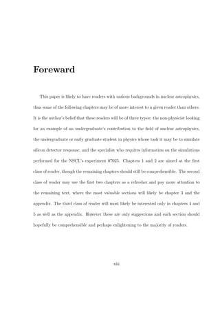
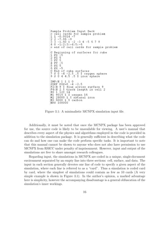
1.4 Produced nuclei expected to reach the detector setup. . . . . . . . . . . . 7
2.1 The Crab Nebula as seen from the Hubble Space Telescope. . . . . . . . 10
2.2 Stellar evolution possibilities. . . . . . . . . . . . . . . . . . . . . . . . . 11
2.3 Artist’s conception of an accreting binary system. . . . . . . . . . . . . . 12
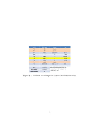
3.1 A minimalistic MCNPX simulation input file. . . . . . . . . . . . . . . . 16
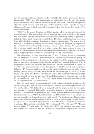
4.1 Near identical initial conditions used for verification simulations. . . . . . 27
4.2 General agreement between MCNPX and GEANT4 verification simulations. 28
4.3 Evidence 976MeV e− can be stopped in 500µm of Si. . . . . . . . . . . . 29
4.4 Engineering drawing of Beta Counting Station[52] . . . . . . . . . . . . . . 30
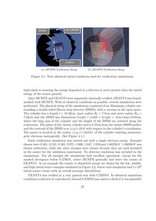
4.5 Formula and schematic for Compton scattering. . . . . . . . . . . . . . . 31
4.6 Experimental data and GEANT4 simulation comparison for validation. . 32
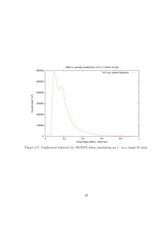
4.7 Unphysical behavior by MCNPX when simulating an e− in a single Si strip. 33
5.1 Experimental set up for experiment 07025 at the NSCL. . . . . . . . . . 36
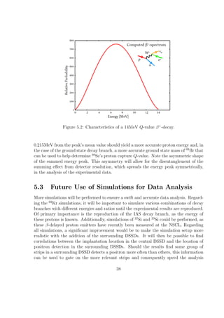
5.2 Characteristics of a 14MeV Q-value β + -decay. . . . . . . . . . . . . . . . 38
69
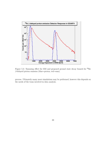
5.3 Summing effect for IAS and proposed ground state decay branch for Kr
β-delayed proton emission (blue=proton, red=sum). . . . . . . . . . . . . 39
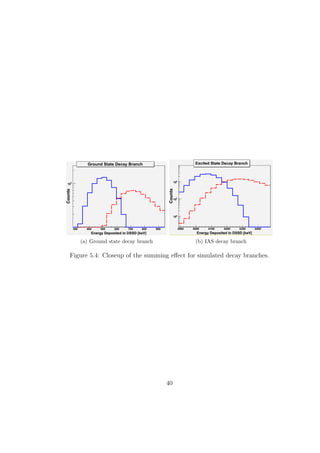
5.4 Closeup of the summing effect for simulated decay branches. . . . . . . . 40
xi](https://image.slidesharecdn.com/thesis-1297292267233-phpapp01/85/BachelorsThesis-11-320.jpg)


![Chapter 1
Introduction to the Study of
Nuclear Reactions
Nuclear physics strives to understand the nuclei of the elements that make up our uni-
verse. The study of nuclear reactions strives to understand how these nuclei interact.
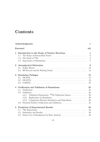
A convenient context in which we speak of nuclei is the chart of nuclides, also known
as a Segr` chart, which is shown in Figure 1.1[1] . The x-axis denotes neutron number
e
N , the y-axis denotes proton number Z, and the combination of these two gives us the
atomic mass A = Z + N . Using these numbers we refer to a nucleus with a given symbol
S with the notation A SN . For example, the ultimate nucleus of interest in this study,
Z
Selenium-68 (A = 68, Z = 34, N = 34), is denoted by 68 Se34 .
34
To describe nuclear reactions, or interactions between nuclei and leptons, we incorpo-
rate our notation for individual nuclei. In a nuclear reaction, the participating particles
that interact are the reactants and the resultant particles after the reaction are the
products. A convenient way to write the reaction is
reactants −→ products.
For this study we’ll deal with one or two reactants and two or three products, so instead
the reaction looks something like
A + B −→ C + D.
Then, to save space, we condense this notation by placing the heavier reactant and the
heavier product, i.e. the nuclei, on the outside of a set of parentheses and place the
lighter reactant and product on the inside of these parentheses, separated by a comma.
So, our fictitious equation above now looks like, A(B, C)D. Often times we will refer to
the outside reactant as the target and the inside reactant as the beam, but in the context
1](https://image.slidesharecdn.com/thesis-1297292267233-phpapp01/85/BachelorsThesis-15-320.jpg)
![Figure 1.1: Chart of nuclides
of a stellar environment it does not really matter which reactant gets which label. In
the physical process that occurs in an astrophysical environment, all that matters is that
the reactants interact to produce the products.
The main factors which control whether or not a nuclear reaction will occur are
the temperature of the environment and the density of reactants in the environment.
A multitude of nuclear reactions are often possible in similar conditions, meaning that
they can occur simultaneously. Thus, we could imagine a situation where our fictitious
reactants A and B can interact along side product C interacting with some other reactant
E.
A + B −→ C + D
C + E −→ F + G
It doesn’t take much of an extension of this idea to realize that whole networks can
form, depleting nuclei of lower mass to build nuclei of higher mass, absorbing and re-
leasing energy along the way. Many such networks exist in astrophysical environments.
The reaction network of interest in this study is the rapid proton-capture (rp-)process.
In the rp-process successively heavier nuclei capture protons (p), releasing energy in
the form of photons (γ). Whenever a nucleus is created that deviates too much from
stability (N = Z for light nuclei), indicated by the black squares in Figure 1.1, this
nucleus undergoes β + decay, where one of its protons changes to a neutron, a positron
(e+ ), and an electron neutrino (νe ). One such piece of the rp-reaction chain looks like [33]
2](https://image.slidesharecdn.com/thesis-1297292267233-phpapp01/85/BachelorsThesis-16-320.jpg)
![34
Cl + p −→ 35 Ar + γ
35
Ar + p −→ 36 K + γ
36
K + p −→ 37 Ca + γ
37
Ca −→ 37 K + e+ + νe .
If the above proton capture reactions are faster than decays on the respective nuclei then
the process can create so called neutron deficient (a.k.a. proton-rich nuclei). Hence the
name “rapid” proton-capture process.
1.1 The Study of Proton-Rich Nuclei
When classifying nuclei each falls into one of three general classes: stable, proton-rich, or
neutron-rich. As you might expect, proton-rich nuclei have more protons than a stable
nucleus of the same mass A and neutron-rich nuclei have more neutrons than a stable
nucleus of mass A. This begs the question, what makes a nucleus stable?
While the nature of stability is much too complicated to be discussed here, it is
worthwhile to briefly consider the simple model for a nucleus. In this model protons
and neutrons, generically known as nucleons, are bound together via the strong force,
which is roughly 100 times stronger than the Coulomb force that causes protons to repel
each other. The bound nucleons must obey the Pauli principle. That is, since they
have half-integer quantum spin, they cannot simultaneously occupy the same spatial and
spin state[3] . Then if space were at a premium, as in a nucleus, it makes sense that it
would be highly efficient, i.e. energetically favorable, to pair protons and neutrons. This
pairing is observed as a tendency for the line of nuclear stability to stay near N = Z
[4]
. Keeping in mind that charged protons repel each other due to the Coulomb force,
it would be expected that at large A more neutrons are added. As a consequence of
the previously stated criterion for a bound nucleus, there are far fewer proton-rich nuclei
than neutron-rich nuclei. But this does not mean proton-rich nuclei are not interesting.
Proton-rich nuclei are the nuclei which are created in explosive hydrogen burning
events, as will be explained in Chapter 2. Hence, it is these nuclei that we must study if
we are to understand the astrophysical events in which explosive hydrogen burning occurs.
While many proton-rich nuclei are created and participate in the rp-process, it would be
incredibly time consuming to study them all. So, given guidance from theoretical nuclear
astrophysicists, experimental nuclear astrophysicists set out to measure the nuclei of
particular importance.
More information will be given in Chapter 2 as to which nuclei are important in the
rp-process, but for the moment we can just refer to these as waiting points. Waiting
points, as the name indicates, are nuclei that delay the flow of the rp-process. This
study will contribute information to the task of finding out how slow one of these waiting
points, that of 68 Se, is. Though there are theoretical predictions, experiment is needed
3](https://image.slidesharecdn.com/thesis-1297292267233-phpapp01/85/BachelorsThesis-17-320.jpg)
![69
Figure 1.2: Proposed level scheme Br.
to verify or falsify the theory. The experiment which this study simulates will add one
piece of the required experimental input.
69
1.2 The Study of Kr
69
Kr (Kr is the symbol for Krypton) is not itself a waiting point nucleus for the rp-
process, but it is key in studying the proton capture of 68 Se. It might then be surprising
that a quick reference of the chart of nuclides, or the periodic table, reveals that the
nucleus one unit of Z greater than Selenium’s Z = 34 is Bromine (Br) with Z = 35,
and not Krypton (Z = 36). However, recalling that proton capture is a process which
transforms nuclei as A SN −→ A+1 TN , it becomes apparent that proton-capture on 68 Se
Z Z+1
creates the (likely) proton-unbound 69 Br[5] . Note that proton capture by 68 Se is still of
interest because reaction rate timescales are short enough in the explosive astrophysical
environments in which the rp-process occurs to allow 69 Br to capture a proton before it
expels the initially captured proton.
Being that 69 Br is too short-lived to allow for study in the lab[6] , we instead exploit
a fortuitous characteristic of 69 Kr. To the advantage of experimental nuclear astrophysi-
cists, 69 Kr undergoes β + -decay to become 69 Br. The decay product is so short-lived, that
the entire decay chain, 69 Kr−→ e+ + νe + 69 Br−→ 68 Se+p is referred to as the β-delayed
proton emission of 69 Kr. In a way that will be outlined in Chapter 5, the light charged
products of this decay chain, e+ and p, are detected with relative ease.
When 69 Kr undergoes β + -decay, it does not necessarily populate the ground state of
69
Br. The “state” refers to the total energy of nucleons within the nucleus. A higher
state has more energy. The binding energy, or energy per nucleon, varies from nucleus to
nucleus. We can determine this energy from a level scheme and, consequently, determine
possible relevant decays. One possible level scheme for 69 Br is shown in Figure 1.2 [7] .
Here the arrows from 69 Kr to levels in 69 Br represent positron emissions of different
4](https://image.slidesharecdn.com/thesis-1297292267233-phpapp01/85/BachelorsThesis-18-320.jpg)
![energies and the arrows from 69 Br levels to 68 Se represent proton emissions of different
energies. It should be noted that of the shown 69 Br levels, only that labeled IAS is
confirmed to exist[5] .
In the experiment which this study (described in more detail in Chapter 5) simulates,
the goal is to identify other levels in 69 Br. Due to experimental limitations, Xu et al.
were only able to identify β-delayed proton emission involving 69 Br’s isobaric analog state
(IAS). As the study was forced to look at a small range in proton energy, they chose to
look at energies that corresponded to the IAS. This is because the majority of β-decays
tend to populate the IAS due to its similar level structure [8] , and indeed Xu et al.
were able to determine 83% of 69 Kr decays populated the IAS. Therefore, other β-decay
branches, and consequently other proton emission branches, can be expected to occur in
the β-delayed proton emission of 69 Kr.
Why not be satisfied with the known decay branch, since it is so dominant? This is
answered simply by relating the excitation energy E of the IAS to its respective tempera-
ture T using the well known relation E ∼ kT , where k is Boltzmann’s constant. Inserting
the IAS energy of 4.07MeV (MeV = 1 million electron-volts) provides the rough astro-
physical temperature necessary to populate this state: T ∼ 1 × 10¹⁰ Kelvin. This over 10
times the typical temperature associated with expected rp-process sites[9] , as shown in
Chapter 2. Given the previously stated information about the levels in 69 Br it is appar-
ent that the levels of interest will be at energies below the IAS and that these levels will
scarcely be populated. More details on the experimental set-up are given in Chapter 5.
1.3 Importance of Simulations
If we could isolate a single 69 Kr nucleus, observe it decay to 69 Br, and then collect
the proton with our detector system, and repeat this process many times over, then
identifying new proton branches would be somewhat trivial. However this simple picture
is far from reality. The first detail to be considered is the time between 69 Kr decaying
to 69 Br and 69 Br emitting a proton. The second concerns the process by which 69 Kr is
produced and delivered to the detector system.
As was stated in the previous subsection, 69 Br is proton-unbound. This means that,
upon coming into existence, it almost immediately expels a proton. The only information
on the lifetime of 69 Br is its non-observation, so that its half-life has an upper limit of
t 1 < 24 nanoseconds[10] . This means that a positron is emitted and detected in our
2
detector system and, on average, less than 24ns later a proton is emitted and detected.
However, the time for the electronics to process information on particles detected so
that the information (e.g. the energy they deposited) can be recorded is of the order of
microseconds[11] . So we must instead gather the information on the positron and the
proton at the same time. This leads to a summing effect that effectively shifts the proton
5](https://image.slidesharecdn.com/thesis-1297292267233-phpapp01/85/BachelorsThesis-19-320.jpg)
![Figure 1.3: NSCL Cyclotrons and A1900 Fragment Separator.
energy peak to higher energies. In order to correct for the β summing effect, simulations
are required to evaluate its impact. Once the shift in the energy distribution peak is
determined, we will be able to more accurately determine the energy of protons emitted
in various decay branches.
Further complications arise due to the 69 Kr production process. Since 69 Kr has a half-
life of 32ms[10] , it must be produced just prior to implantation in the detector system.
The process in which it is produced is called fragmentation. In fragmentation a heavy
isotope, here 72 Kr, is accelerated as the primary beam and collided into a production
target, here Beryllium. These collisions produce many different kinds of isotopes, occa-
sionally producing our nucleus of interest. A series of magnets, here the A1900 Fragment
Separator (See Figure 1.3[30] ) then separates out the nucleus of interest, but often the
process is imperfect and other nuclei make it to the detector system. The simulation
will only simulate the processes of interest, i.e. β-delayed proton emission, thus it should
help in discerning relevant data from the whole.
One may wonder how it can be known that simulations are accurately reproducing
the physical conditions of the experiment. This subject is discussed some in Chapter
3 and at length in Chapter 4. The main simulation of this project and the experiment
it simulates are detailed in Chapter 5. How this simulation will be used to aid in the
interpretation of the experimental results follows this in Chapter 6.
6](https://image.slidesharecdn.com/thesis-1297292267233-phpapp01/85/BachelorsThesis-20-320.jpg)

![Chapter 2
Astrophysical Motivation
Since ancient times humans have been intrigued by the lights that illuminate their night’s
sky. For those observing before the invention of telescope, these objects were simply
unchanging points that were static with respect to each other. Once in a very long while
a new light would appear, often shining throughout the day, and then slowly fade out of
existence. The Crab Nebula (see Figure 2.1[15] ) is a well known example of one of these
transient lights in the night sky that the Chinese observed in 1054AD. These occurrences
offered the first clues that these lights were much more than decorations on the ceiling
of the celestial sphere.
With the invention of the telescope astronomers were able to analyze the lights of
our night sky more detail. The introduction of the fields of spectroscopy, the study of
light’s interaction with matter as a function of wavelength, and spectrometry, the study
of the creation and absorption of light due to atomic and nuclear structure, empowered
astronomers with the quantitative capabilities they have today. Applying these two
disciplines, Suess and Urey [16] were able to determine the relative abundances of the
nuclei in our solar system. One year later Burbidge, Burbidge, Fowler, and Hoyle[17] ,
and separately Cameron[18] , used this information and that from the then 20 year old
field of nuclear physics to propose how all of the nuclei in the universe were synthesized.
Thus nuclear astrophysicists were provided one of the major foundations of the field.
Nuclear astrophysics studies the synthesis of elements in stars and stellar environ-
ments and their dispersion into the interstellar medium. It provides us with unique
insight into the building blocks of nature, allowing us to study nuclei in environments
that are only marginally reproducible on earth. Volumes could be (and have been) filled
on the many nucleosynthesis sites extant in our universe, but the remaining discussion
will focus on the main site that is pertinent to this study. This is the astrophysical site
known as a type-I x-ray burst.
9](https://image.slidesharecdn.com/thesis-1297292267233-phpapp01/85/BachelorsThesis-23-320.jpg)
![Figure 2.1: The Crab Nebula as seen from the Hubble Space Telescope.
2.1 X-Ray Bursts
Type-I x-ray bursts are frequently recurring thermonuclear (driven by temperature de-
pendent nuclear reactions) explosions on the surface of an accreting neutron star’s crust[19] .
They were first observed in the early to mid-1970s [20][21] , characterized by a steady peak
flux of light in the x-ray region (0.01nm ≤ λ ≤ 10nm) with an occasional sharp rise in
luminosity followed by an exponential decay. Astrophysics theorist produced sugges-
tions as to their underlying cause shortly after a multitude of these observations were
published[22][23][24] . The essence of these models involves a binary star system in which
a neutron star and a main sequence or giant star revolve around each other, as in Figure
2.3.
A neutron star is an extremely dense body, mostly composed of neutrons, left behind
from a massive star’s core-collapse explosion, known a type-II supernova. Main sequence
stars synthesize helium from hydrogen in their cores, but are mostly hydrogen. Giant
stars have evolved off the main sequence, having burned through most of their core
hydrogen, and have an outer envelope made mostly of hydrogen and helium. All stars
begin as main sequence stars and evolve into giant stars. Those that are roughly 8 times
the mass of the sun (8M⊙ ) and above eventually become type-II supernova. The main
paths taken in stellar evolution are shown in Figure 2.2[25] . For a typical x-ray bursting
system the neutron star is a roughly 1.4M⊙ supernova remnant and its companion is a
giant star of order 1M⊙ or less.
In an x-ray binary system giant star is transferring gas to the neutron star in a process
called “accretion”. Mass transfer is possible because the giant star has expanded so that
10](https://image.slidesharecdn.com/thesis-1297292267233-phpapp01/85/BachelorsThesis-24-320.jpg)
![Figure 2.2: Stellar evolution possibilities.
its gas fills its Roche lobe while overlapping the neutron star’s Roche lobe. The Roche
lobe is essentially sphere in which a star’s mass is gravitationally bound [26] . Once mass
transfer is initiated gas flows freely from the surface of the giant star to the surface of the
neutron star, as shown in Figure 2.3[27] . As a result of accretion, gas rich in hydrogen
and helium builds up on the crust of the neutron star. This results in the emission of
x-rays due to the gravitational energy released during accretion in all of these systems
and nearly half also undergo in type-I x-ray bursts [28] .
Due to the system’s steady emission of light which peaks in the x-ray portion of
the spectrum, astrophysicists can infer the temperature of the environment via the well
known relations
hc
E= ∼ kT
λ
(4.1 × 10⁻²¹ M eV ∗ s)(3. × 108 m/s)
T ∼ −9 −11 ∼ 1. × 108 K,
(0.1 × 10 m)(8.6 × 10 M eV /K)
where k is Boltzmann’s constant, h is Planck’s constant, and c is the speed of light. A
6 6
more realistic approach utilizes Wien’s displacement law, T = 2.9×10λnm∗K = 2.9×10 nm∗K =
0.1nm
2.9 × 10⁷ K. While this allows us to calculate the temperature at the surface of the burst-
ing site, this temperature must be related to the temperature of the bursting zone via
models. In general models infer the thickness of a burning layer by calculating how many
nuclei, each releasing roughly 5MeV of energy in a given fusion reaction, it would take
to create the observed energy of ∼1038 erg . Observational indications that the site is a
sec
11](https://image.slidesharecdn.com/thesis-1297292267233-phpapp01/85/BachelorsThesis-25-320.jpg)
![Figure 2.3: Artist’s conception of an accreting binary system.
neutron star, which are beyond the scope of this paper, can be included to arrive at the
general conditions for an x-ray burst that can be included in simulations.
Why study x-ray bursts? From a statistical point of view x-ray bursts are unique
astronomical objects in that over 1,000 have been observed from over 40 separate sites
[29]
. We are thus able to see how bursts vary between binary systems and how the bursts
vary within a single system’s recorded bursting history. This allows for the identification
of common features and dependencies of the bursts on things such as the giant star’s
mass, the giant star’s composition, and the rate of accretion. In astronomy such a robust
data set is very rare, meaning that x-ray bursts are invaluable sources of information.
X-ray bursts have the potential to be a wealth of physics information, though much
work must still be put into understanding them before that wealth can be exploited. Of
particular interest is the nuclear physics of x-ray bursts that provides input regarding
the neutron star’s radius and its crustal composition. Each of these allows us to learn
about the neutron star structure, which provides information about the equation of state
of dense nuclear matter and consequently about the strong nuclear force [30] . Observing
the effects gravitational redshift has on the thermal emission spectrum of matter being
accreted onto the neutron star provides information on its mass to radius ratio and
studying the final abundances of nuclei produced by the rp-process indicates what the
crustal composition neutron star would be[19] . However, we will not be able to extract
these parameters with the necessary level of confidence until we have improved our models
of x-ray bursts[31] , which are very sensitive to nuclear physics data [32] . Currently one
of the main ways to determine which nuclear physics data is of particular importance in
x-ray bursts is to determine which data are important in the rp-process.
12](https://image.slidesharecdn.com/thesis-1297292267233-phpapp01/85/BachelorsThesis-26-320.jpg)
![2.2 RP-Process and Its Waiting Points
The rp-process is a mechanism of nucleosynthesis in which protons are captured on nuclei
to create successively heavier proton-rich nuclei. Proton capture can be stalled when a
nucleus is reached whose proton capture rate is prohibitively small so that it must undergo
β + -decay for the process to continue[33] . The nuclei that cause this occasional stalling
are especially interesting because differences in the time the rp-process waits there can
cause a large difference in the final abundance of nuclei produced [19] . These nuclei
are called “waiting points”. Nuclear physics data combined with nuclear astrophysical
models allow us to determine which nuclei are waiting points.
Before the rp-process is initiated, the x-ray burst begins due to thermonuclear run-
away, a process in which a reaction that is highly sensitive to temperature releases energy,
increasing the temperature, thereby increasing the reaction rate and providing positive
feedback [26] . Here runaway is triggered due to the highly temperature sensitive triple-
alpha reaction, which ultimately synthesizes 12 C from three 4 He (a.k.a. α). Temperatures
then rise to initiate α-capture which then provides the energy and seed nuclei necessary
to initiate hydrogen burning for the rp-process [34] . The exact path of the rp-process
is highly dependent on temperature and density, particularly regarding capture on light
nuclei due to competition with α-capture induced reactions, but above calcium the rp-
process is only determined by proton captures and β-decays[33] . For nuclei in this region
along the proton drip line, the rp-process is dominated by β-decay lifetime of waiting
point nuclei [33] . Thus if the process were able to bypass a waiting point nucleus via a
proton capture, the path of the rp-process, and consequently the light curve and final
composition of the x-ray burst, could be significantly altered[35] .
Of the high A nuclei on the rp-process, one that has been identified as a waiting
point, from β-decay measurements, is 68 Se. However, uncertainties remain in calculating
the proton capture reaction rate, so it is possible that successive capture of two protons
could allow the rp-process to bypass 68 Se [19] . The issue then is to determine these proton
capture rates on earth.
When studying nuclei that are proton-rich we have seen that are short-lived. Being
that they do not maintain their current proton-rich state for very long, it is apparent that
adding a proton to one of these nuclei is not a simple task. So, to circumvent this issue,
we instead study the opposite process. Here this means we study the proton emission of
69
Be instead of the proton capture by 68 Se. Though the rates for these processes are far
from equivalent, the nuclear structure is the same. As the mass difference, given from
nuclear structure, between 69 Br and 68 Se is the most important variable in determining
the proton-capture Q-value, we attempt to determine 69 Br’s ground state mass. We de-
termine this mass by detecting the energy of protons resulting from 69 Br proton emission,
which we study by necessity via the β-delayed proton emission of 69 Kr. The method of
determining this structure is detailed in Chapter 5.
13](https://image.slidesharecdn.com/thesis-1297292267233-phpapp01/85/BachelorsThesis-27-320.jpg)

![Chapter 3
Simulation Packages
The physics of charged particle interactions in detector systems involves many processes
that are highly sensitive to incident energies, occur on small timescales, and involve small
spatial scales. As a result, modeling this physics requires a simulation code that is able
to take into account large and varied data and implement this data with the smallest
possible spatial and temporal resolution. While creating a personal simulation package
for such physics is not out of the question, the process would require years of effort to
ensure a properly working code. Thus, to avoid reinventing the wheel, it is often more
practical to employ previously tested and developed simulation packages.
The simulation packages used here were Monte Carlo N-Particle X (MCNPX)[36] ,
Geometry and Tracking 4 (GEANT)[37] , and Monte Carlo Simulation of Electron Tra-
jectory in Solids (CASINO)[38] . Each of these packages is the result of over a decade of
development and testing. Also, each is relatively easy to acquire, though MCNPX takes
some extra effort. GEANT4 was the primary simulation package used and MCNPX and
CASINO were used to verify its results. The following sections will attempt to briefly
explain the uses and methods of simulation for each package.
3.1 MCNPX
MCNPX is a simulation package developed by Los Alamos National Laboratory which
has major updates roughly every 3 years [36] . The version used in this study was MCNPX
2.6.0 (package ID:C00740MNYCP02), originally released in April 2008. A copy of this
software can be obtained by contacting the Radiation Safety Information Computational
Center (RSICC)[39] . However, as MCNPX is a product of the United States Department
of Energy, it requires paperwork to be submitted and it is advisable that contact with
RSICC is initiated by a laboratory or university software representative. The entire
process can take anywhere between two weeks and one month before the software is in
hand.
15](https://image.slidesharecdn.com/thesis-1297292267233-phpapp01/85/BachelorsThesis-29-320.jpg)
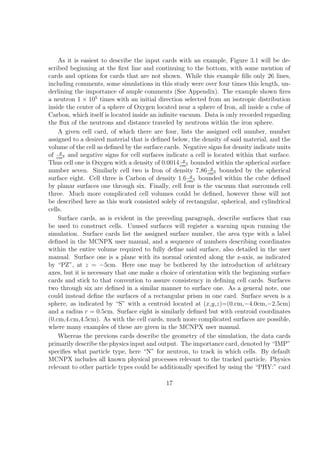
![possible, however one should consult the MCNPX user manual for such cards.
To produce output, one must first source the MCNPX package software with the
command “source /filepath/”. The simulation is then run with the command “mcnpx
i=InputFilename o=OutputFilename. Additional commands can be appended to this
line for a more customized output. Of particular use in the debugging phases is the
option “PRINT”, however this should not be used for long (> 1e4) simulations as it
creates a large output and consequently slows runtime. Visual output, also invaluable in
debugging, can be created by loading input files into the VISED[40] software, however
this too must be obtained from RSICC.
The output of the MCNPX simulation contains many pieces of information, most
are of little interest here, so an attempt will be made to briefly highlight important
output quantities. The basic structure of the output is as follows: restate the input,
describe the input geometry, describe the specified source, list physical characteristics
of initial group of Monte Carlo simulations, list results of “F” tallies as binned by “E”
tallies, list statistical qualities of recorded tallies, and list the total simulation time in
human units (e.g. actual minutes). A sample output is not pictured here due to its
excessive length, e.g. 300 lines for the simple input shown. As was stated,a more verbose
output can be printed, and should be during debugging phases, using the “PRINT”
option. Additionally, warnings will be listed after the listed physics input or output that
MCNPX developers think generally require special attention. In practice the output
initially requires a close reading with the MCNPX manual in hand, so no effort will be
made to describe it any further. Output from simulations performed in this study is not
listed in the appendix due to size, however the author can be contacted if one wishes to
consult a full output file of a simulation presented.
3.2 GEANT4
GEANT4 is a simulation package developed by users of the CERN facility[41],[42] and is
maintained by the its user community. The installation used here was version 9.1.0, which
was released in January 2008. GEANT4 software is freely available online, provided one
is able to download a roughly 0.5Gigabyte file. As the code is open source, one is freely
available to inspect and alter source code with the caution that the software has been
developed and inspected by hundreds of professionals.
GEANT4 simulations are coded modularly in a C++ style language, where hundreds
of pre-made classes contained in the original software are available for use. General
knowledge of C++ syntax is not required to create GEANT4 simulations, but it is highly
recommended. An attempt will be made here to describe the general make-up of a simple
GEANT4 simulation, however due to the modularity of the code the following description
will certainly lack the clarity of that given in the section on MCNPX. All codes described
19](https://image.slidesharecdn.com/thesis-1297292267233-phpapp01/85/BachelorsThesis-33-320.jpg)
![will be located in the appendix.
Regarding general modules of the simulation, a main code is run that contains ref-
erences to the header files of the primary components of the simulation. These primary
components are main geometry, materials used, physics processes included, method in
which a single simulation iteration is generated, and method in which desired data is
recorded. Each header file contains definitions of included classes as well as references to
minor components of the simulation that specify things such as an individual detector’s
geometry or a special method of tracking data in a particular component of the simu-
lation. Header files have a corresponding source file which contains instances of classes
defined in the headers. Generally the main code exists in a directory above two sepa-
rate directories, include which has the header files and src which has the source files.
Throughout the code references are often made to predefined classes that contain infor-
mation such as a method of specifying a given geometry or an algorithm to sample a
Gaussian distribution. Other than this, no pieces of physics, input, or output are pro-
vided for the user. As such, the author advises that one begin by working by inspecting
and imitating working examples, using references such as the GEANT4 User Support
[43]
and the doxygen GEANT4 documentation [44] .
The main code is the driver for all other codes. It initializes the conditions of the
simulation by calling the main modules of the simulation. The driver constructs the
simulation volume, initializes the method of outputting the results, initializes the physics
to be included, initialize the visualization method, initialize the method of generating
a given simulation event, and finally the simulation event is run. The simulation is
compiled such that it handles a single event. The compiled code is iterated over for a
user-specified number of events by a compact macro that will be described after main
code components.
Construction of the volumes within the simulation is generally done by a code called
DetectorConstruction, or something similar to this. Within this code each physical com-
ponent of the desired simulation is constructed and oriented within an arbitrarily defined
“world volume”. It is generally more convenient to reference the components of the sys-
tem via separate modules so that one could swap, say, a cylinder made of aluminum
with a rectangle made of lead, by changing a few lines of code. For each component
constructed, a material is specified to fill the volume, the volume itself is specified via
some shape and central coordinates, and an associated “messenger” class is called. A
messenger class is necessary for any volume through which the particle of interest might
pass on its way to a volume of interest, much like the “IMP” card in MCNPX. Ad-
ditionally, for volumes that are detectors which will ultimately “detect” your particle,
as the double-sided silicon strip detector in this study, the volume must be specified as
“sensitive”. Sensitive volumes require an additional code that specifies what and how to
track in said volume.
The method of recording and outputting of results is varied and very loosely defined in
20](https://image.slidesharecdn.com/thesis-1297292267233-phpapp01/85/BachelorsThesis-34-320.jpg)
![GEANT4 documentation. The results code must interface with the code that generates
the initial source particles as well as the code for the sensitive detector. (The code used
here, Results, was based on work by Ron Fox.) In this code a hexadecimal value is
assigned to variables that indicate the type and initial energy of source particles and the
type and energy of particles that impact a sensitive detector. Prior to printing the string
of assigned variables for an event to an output file, a variable is written indicating the
beginning of an event and, after the string of variables, a variable is written indicating
the end of an event. This data is sorted into a ROOT readable format by a code that will
be described after the description of the macro that runs the simulation. Note that one
does not necessarily need to output results in the same manner as described here, but
some method must be employed if one is to go beyond simply visualizing the simulation
results.
The physical processes to be included in a simulation are contained in the code called
something like PhysicsList. Here the processes in which a source particle can interact
with a detector system are individually listed for each potential particle of interest. For
certain particle types, like the electron, special “low energy” (< 1MeV) processes can be
employed. The processes are assigned an order to be evaluated and some are executed
only once a particle has dropped below a given kinetic energy. For example, when simu-
lating a positron in this study, included are scattering, ionization, bremsstrahlung, and,
only once the positron is “at rest”, annihilation. During a single event of a simulation the
particle will move along in steps with the direction of motion being decided in a proba-
bilistic (but physical) manner and whose length are specified in GEANT4 documentation
(but are changeable). Certain types of processes, e.g. scattering and ionization, can hap-
pen at substeps of a given step, while others, e.g. bremsstrahlung, only occur after a
step. Additionally, one can specify here at what energy to effectively stop a given par-
ticle or simply choose to accept default values. (Here default values were used because
a positron is stopped at 1keV, however the detector thresholds in the actual experiment
are no lower than 70keV.)
As with simulation results, the method of visualization varies widely amongst GEANT4
codes. Here the package VRMLview[45] version 1.0 was used. This package is not nec-
essarily recommended, particularly as it is from 1997, however it was used in this study
because it was available. Regardless of the package employed, a code generally named
VisManager initializes the graphics system and allows it to communicate with the simu-
lation as it runs. Creation of a visualization can be turned on or off in the compact macro
that runs the simulation. It is advisable to not create visualizations for simulations of
more than 1,000 events unless a computer with considerable processor power is employed.
Source particles are emitted (“fired”) by a code generally named something like Pri-
maryGeneratorAction. This code specifies all of the characteristics of the source. Here a
source can be as simple as a monoenergetic electron fired in a single direction, or it can
be made to fully replicate an actual radiation source. If the latter is chosen, one must
21](https://image.slidesharecdn.com/thesis-1297292267233-phpapp01/85/BachelorsThesis-35-320.jpg)
![code all source particles, energies, and their respective probabilities of emission. When
choosing this option it is wise to consult the National Nuclear Data Center (NNDC)[46]
and to be sure to include only decay branches that have a statistically significant proba-
bility of occurring during the total number of simulations run. Regardless of the source
chosen, one can specify the initial position of the source as well as the direction in which
to fire the source particle, where each could be chosen probabilistically.
To compile the code, one must first source the GEANT4 library with the command
“source env.sh”. evn.sh and env.csh are two files which exist in the same directory
as the driver. These files contain information on how to compile the GEANT4 code.
Before the code is executed one must ensure that their .bashrc file contains the command
“export G4WORKDIR=/filepath.” One then runs “make clean”, “make”, and finally
“./ExecutableName”. At this point a compact code for a single simulation as been created
which typically shares the name of the executable file, but lacks the file extension.
The full simulation is finally run using a compact macro, here my vis.mac. This is
a short code, typically 10s of lines long, in which it is specified how verbose the output
of the simulation should be, whether or not to create a visualization, and how many
simulation events to perform. The full Monte Carlo simulation is then run with the
command “./ExecutableName CompactMacro OutputFile”. The contents of the output
file are specified by the results code.
For analysis it is desirable to convert the output into a ROOT[47] -readable format.
(There are likely many ways to do this, however the author simply followed an example
created by Ron Fox.) This code, generically called something like Sort2Root, initializes
a ROOT Tree, its Branches, and their Leafs to bin the data from the OutputFile into
histograms that can be used in analysis. Additionally, this code can be used to apply
detector-like resolution by effectively smearing out data bins with some desired distribu-
tion. Here this was done by taking each event energy as the centroid of a Gaussian and
using the weighted probability of the Gaussian to select a new energy, finally putting the
event into the corresponding new energy bin. Prior to writing such a code it is advisable
that one gain some familiarity with the ROOT software. Examples of all of the previously
described code will be included in the appendix as they looked for the final performed
simulations. Source code for simpler versions are also available if one wishes to contact
the author.
3.3 CASINO
CASINO is software created to model the trajectory of electrons in solids, particularly for
situations involving Scanning Electron Microscopoes (SEM)[48] . The code was developed
by the research teams at the Universit´ de Sherbrooke[38] and is freely available for
e
download online, provided one register for permission on their website. The full source
22](https://image.slidesharecdn.com/thesis-1297292267233-phpapp01/85/BachelorsThesis-36-320.jpg)


![Chapter 4
Verification and Validation of
Simulations
In order to properly interpret the results of any experiment in nuclear physics, it is often
necessary to have an accompanying simulation. Simulations provide insight into the
involved physical processes and they provide a laboratory in which one can freely change
experimental conditions and visualized their impact on the results. Here the simulation
is required to correct the observed particle energy for β-summing to extract the correct
proton energy. However, before a simulation can be used it must be extensively tested to
ensure it provides results that replicate the system of interest. The processes of testing
a simulation are known as verification and validation.
Verification is ensuring that a code accurately reproduces the desired theoretical
model being used to describe a physical situation. Validation is ensuring that the cho-
sen physical model accurately represents the physics of the situation of interest[49] . In
verifying a code one uses methods such as plausibility checks, back of the envelope calcu-
lations, rigorous examination of output for known cases, echoing of input upon output,
and comparison with codes made for a similar purpose. In validating a code one per-
forms a controlled, usually simple, experiment whose results are robust and compares the
experimental results to those of a simulation replicating that experiment. The actions
taken to verify and validate the simulations presented in this study are given below.
4.1 Verification
Verification has two main classes: internal verification and external verification. Internal
verification checks the output of a given code against its input to ensure the desired
model was properly simulated. External verification, or benchmarking, compares the
results of simulations performed with separate codes that have identical, or as identical
as possible, conditions. Internal verification was performed here for the MCNPX and
25](https://image.slidesharecdn.com/thesis-1297292267233-phpapp01/85/BachelorsThesis-39-320.jpg)
![(a) 0.481MeV e− (b) 1.000MeV e− (c) 1.682MeV e−
Figure 4.2: General agreement between MCNPX and GEANT4 verification simulations.
that electrons of a given energy could be stopped in Silicon of a given thickness. To
mimic the DSSD, the material chosen in the CASINO verification simulation was 500µm
of Silicon. The initial electron energy was chosen to be 975keV, as this is the energy of
primary importance in the validation experiment, and the initial angle was chosen to be
50◦ , admittedly an extreme case. This simulation confirms that some of these electrons
can and are stopped in the Silicon, as is shown by the energy deposited by depth in
Figure 4.3. Here it is shown that 90% of the electron’s energy are deposited within the
red contour when an electron enters the Silicon at an angle of 50◦ , well within a depth
of 500µm, the thickness of the DSSD. (A useful paper for interpreting CASINO plots is
[50].)
4.2 Validation
207
4.2.1 Validation Experiment: Bi Calibration Source
Validation was performed using an experiment whose basic setup was identical to that
described for the verification simulations. The source used was 207 Bi which predominantly
emits electrons with energies 0.481, 0.553, 0.565, 0.976, 1.048, 1.059, and 1.682MeV with
probabilities 13.1, 3.8, 1.3, 60.9, 16.0, 4.7, and 0.2%, respectively[46] , where probabilities
are normalized to only include these electrons. Electron energies which 207 Bi also emits
were not included due to their small probability of emission. For example, the most
frequent electron energy that was not simulated is MeV, which is emitted once in every
2 × 10³ times the 976keV electron is emitted. (See [46] for a full characterization of the
source). The DSSD, a type “BB1” purchased from MicronSemiconductor[51] , was held
up by four aluminum rods which extended from one of the cylinder end caps. The data
collected was relative energy deposited by electrons in the DSSD, which was recorded
28](https://image.slidesharecdn.com/thesis-1297292267233-phpapp01/85/BachelorsThesis-42-320.jpg)
![Figure 4.3: Evidence 976MeV e− can be stopped in 500µm of Si.
by collecting electron-hole pairs created as the electron passed through the Silicon. A
voltage of 50V was applied across the detector so that charges from all parts of the
detector could be collected. An engineering drawing of the actual setup, without the
surrounding cylinder, is shown in Figure 4.4.
4.2.2 Replication via Simulation
In the simulation many simplifications were made, however it seems they are justified.
Source energies mentioned in the previous subsection are not all of the electron energies
emitted by 207 Bi, however other physical energies are emitted with a relatively low proba-
bility. Additionally 207 Bi emits photons, but it was found these do not significantly affect
the energy spectra. A full characterization of 207 Bi can be found at [46]. As is apparent
from comparing Figure 4.4 and 4.1, numerous approximations were made in creating the
simulation geometry. Ultimately only the Aluminum cylinder and the DSSD were in-
cluded because it was found that backscattering of electrons off the Aluminum chamber
had little impact on simulation results. So it was then assumed that the aluminum rods
supporting the DSSD would have an even smaller effect.
29](https://image.slidesharecdn.com/thesis-1297292267233-phpapp01/85/BachelorsThesis-43-320.jpg)
![Figure 4.4: Engineering drawing of Beta Counting Station[52] .
4.2.3 Comparison Between Simulation and Experiment
In order to compare data from the validation experiment and simulations of that ex-
periment, a calibration had to be performed to the DSSD. This was necessary because
the energy that is recorded is relative and is binned into “channels”. Channel to energy
calibration was performed by M. del Santo by recording the channels the recorded energy
deposition for several sources of known energy. M. del Santo additionally performed a
calibration using Compton scattering. Here photons from a source that mainly emits a
photon of a given energy is allowed to pass through the DSSD and is detected afterward
by a germanium detector. The change in the photon’s angle and energy is sufficient to
obtain the energy imparted to the detector, as is shown schematically in Figure 4.5.
The channel to energy calibration ultimately resulted in a 4th order polynomial func-
tion that could be applied to the data. Adjustments were also made to the gain applied
to the data and the total number of simulation events was designed such that the total
number of recorded events would match the data. The resulting calibration function
applied to the data in the presented results was
Energy(x = Channel) = G ∗ (p0 + p1 ∗ x + p2 ∗ x2 + p3 ∗ x3 + p4 ∗ x4 ), (4.1)
where, to two decimal places, G = 8.6 × 10² and p0,1,2,3,4 = 0.0, 4.90 × 10⁻³ , 2.02 ×
10−4 , −6.94 × 10⁻⁷ , and 8.15 × 10⁻¹⁰ , respectively. The GEANT4 simulation used for
comparison had 1 × 10⁵ source events, but the resulting data bins were multiplied by a
factor of 25 to have the same overall counts. The resulting comparison is shown in Figure
4.6.
30](https://image.slidesharecdn.com/thesis-1297292267233-phpapp01/85/BachelorsThesis-44-320.jpg)
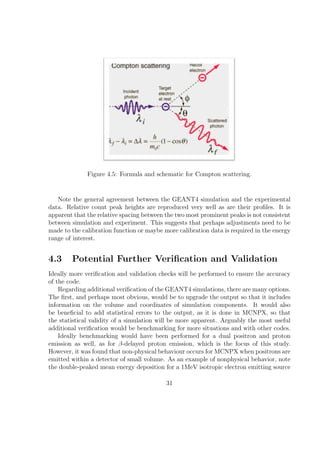
![Figure 4.6: Experimental data and GEANT4 simulation comparison for validation.
centrally located within in a DSSD shown in Figure 4.7. These simulations could not
be performed with CASINO as it only simulates the trajectory of electrons in materials.
For benchmarking this type of physics, the author has recently become aware of the
FLUKA[55],[56] simulation package, which seems well suited due to its versatility and
well developed user support.
Regarding additional validation, any number of experiments could be performed. The
most useful experiments would use another discrete electron source or an alpha source
or a proton beam. An alpha source was not simulated in this study. Being that the
proton, for which the alpha calibrates, is generally fully stopped within the DSSD, it was
assumed here that the centroid of its energy distribution would be centered around its
full energy with a full width half maximum of the detector’s resolution. As experimental
information provided this full width half maximum, it seemed unnecessary to perform
a simulation to confirm this result as the full width half maximum of detector response
is given to the simulation as input. A proton beam was not simulated because it seems
unlikely that the DSSD will be taken to a facility with a proton beam in the near future.
32](https://image.slidesharecdn.com/thesis-1297292267233-phpapp01/85/BachelorsThesis-46-320.jpg)

![Chapter 5
Prediction of Experimental Results
Prior to describing the experiment and simulation that were the focus of this study,
the purpose will be briefly rehashed. Recall that the goal is to identify levels in 69 Br,
particularly the ground state, that lay below its isobaric analogs state (IAS). The proton
emitted from the ground state of 69 Br is of particular interest because it will allow us
to determine a ground state mass for the nucleus, which can be used to experimentally
assign a proton capture Q-value to the rp-process waiting point nucleus 68 Se. The method
which will be used to measure the proton’s energy is the detection of β-delayed proton
emission by 69 Kr, which will inherently sum the energy of the emitted positron with the
energy of the proton, upon detection. The experiment being described to accomplish this
task is scheduled to be performed by Marcelo del Santo, accompanied by the research
group of Hendrik Schatz, from May 10 to May 18 (roughly one week from this writing)
as experiment 07025 at the National Superconducting Cyclotron Laboratory (NSCL).
69
5.1 Kr Experiment
As 69 Kr has a half-life of t 1 = 32ms[46] , it must be produced on site at the NSCL. An ion
2
source produces 78 Kr, which is accelerated by the coupled K500 and K1200 cyclotrons[57] ,
schematically shown in Figure 1.3, to an energy of 150 Mu (MeV per Nucleon). At 25
eV
particle-nanoamps (pnA), the beam will be fragmented by a Beryllium target to produce
69
Kr and along with some contaminants. Most of the contaminants will then be removed
as the beam passes through the A1900 fragment separator[30] and the Radio Frequency
Fragment Separator[58] (RF Kicker). Finally the beam will pass through three single
sided PIN Silicon detectors and one DSSD, implanting 69 Kr in a second DSSD which has
behind it a third DSSD and a fourth PIN detector. Collectively these Silicon detectors
are the Beta Counting Station (BCS)[52] . This is shown schematically in Figure 5.1. Not
shown is the Segmented Germanium Array (SeGA)[59] which will surround the BCS.
35](https://image.slidesharecdn.com/thesis-1297292267233-phpapp01/85/BachelorsThesis-49-320.jpg)
![Figure 5.1: Experimental set up for experiment 07025 at the NSCL.
The data of primary interest in the experiment is the energy deposited in the BCS
and SeGA. The BCS will collect energy from positrons and protons resultant from 69 Kr
β-delayed proton emission and SeGA will collect energy from photons emitted in the
de-excitation of 69 Br. As each system will also detect radiation from background and
contaminants, gates have been devised so that events having decay signals in the BCS
and SeGA in coincidence can be isolated so as to effectively remove the majority of
contaminants and background for decay branches that pass through an excited state
of 69 Br. For the ground state decay branch one would not expect a photon. Working
from the assumption that said gating will be effective, the simulation in this study only
examines the effects of radiation from β-delayed proton emission in the BCS.
5.2 Simulation and Results
As was the case for the validation experiment, simplifications were made to approximate
the system of interest. Indeed the setup simulated here is identical to that described in
section 4.2.2 and shown in Figure 4.1, with the only difference being the source and its
location. Here the source is located within the DSSD and emits a positron and then a
proton, so as to replicate β-delayed proton emission of 69 Kr. A time delay between the
positron and proton emission is not included, as this time in reality will be undetectable
using the given experimental setup.
Any number of decay branches could have been simulated, however here we only
examined the decay through the IAS and the lower limit for the ground state of 69 Br.
The IAS branch was chosen because it has been previously observed[5] . The ground
36](https://image.slidesharecdn.com/thesis-1297292267233-phpapp01/85/BachelorsThesis-50-320.jpg)
![state decay branch was simulated because extracting its energy is the main goal of the
experiment and the lower limit was chosen because it provides the lowest energy signature,
closest to detector threshold, we expect to detect.
The simulation goes through the IAS branch 83% of the time, as this was the branch-
ing ratio assigned by [5]. Upon selecting the decay branch, the rejection method[53] is
used to select the energy of the emitted positron according to its β-spectrum, which is
defined by the decay’s Q-value. Recall that the positrons can have different energies for a
decay of a given Q-value because β-decay is a three-body reaction and thus the positron
and electron neutrino may divide the total available kinetic energy differently each time
(see Figure 5.2). The β-spectrum was calculated using the simple relation[4]
dPE dp
dE
= ξ ∗ dP ∗ dE
dp
dPE
dE
= ξ ∗ p2 ∗ (Q − E)2 ∗ dE
dp
dPE 2
dE
= ξ ∗ p ∗ (Q − E) ∗ (E + me )
where PE is the probability of emitting a positron of a given kinetic energy, E is an
energy selected randomly from E = 0 to E = Q, Q is the Q-value of the decay, p is
the momentum, me is the mass of a positron, and ξ is a normalization constant[4] that
contains cancelling units and brings the maximum probability to 1. If PE is greater
than a random number selected from 0 to a number greater than Pmaximum then the
positron is fired with energy E. A Coulomb correction factor[54] could have been added,
however this would require integration of the probability distribution each event and,
upon comparison, the distribution was negligibly different for the purposes of this study.
Following positron emission, a proton is emitted with an energy in accordance to the
decay branch chosen. Thus, roughly 83% of the time a positron will be emitted with with
an energy defined by a 10.069MeV Q-value, followed by a 4.07MeV proton, and the rest
of the time a positron will be emitted with an energy defined by a 14.019MeV Q-value,
followed by a 0.50MeV proton.
The simulation result that was primarily investigated was the total energy deposited
in the DSSD in a decay event compared to the energy deposited only by the event’s
proton. More specifically, the comparison made was the difference between the centroids
of the peaks for these energy deposition distributions, as this is the information used to
correct for the summing effect. For the results shown (see Figures 5.3 and 5.4) the energy
deposited was segmented into 0.035MeV bins and a detector resolution of 0.175MeV,
experimentally determined by M. del Santo, was applied at all energies.
One can see that the shift in the centroid of the energy deposition distribution due
to β + summing is 0.215MeV for both decay branches. This result indicates that this
shift will apply to all detected protons. Consequently, it seems unnecessary to simulate
additional decay branches until the experiment is performed. Once peaks in energy
deposition from β-delayed proton emission are identified in data analysis, subtracting
37](https://image.slidesharecdn.com/thesis-1297292267233-phpapp01/85/BachelorsThesis-51-320.jpg)
![Bibliography
[1] http://www.phy.ornl.gov/hribf/science/abc/
[2] Van Wormer, L. et al. Astrophysical Journal. 432 (1994), 326
[3] Gottfried, K. & Yan, T. Quantum Mechanics: Fundamentals. New York: Springer-
Verlag, 2003
[4] Martin, B. Introduction to Nuclear Physics. West Sussex, United Kingdom: Wiley &
Sons, 2009
[5] Xu, X.J. et al. Physical Review C. 55 (1997), 2, R553
[6] Lima, G.F. et al. Physical Review C. 65 (2002), 044618
[7] Schatz, H. et al. Private Communication
[8] Kramer, K. Introductory Nuclear Physics. Hoboken, New Jersey: Wiley & Sons, 1988
[9] Schatz, H. et al. Physics Reports. 294 (1998), 167
[10] Tuli, J. NNDC 2007 Nuclear Wallet Cards http:://www.nndc.bnl.gov/wallet
[11] Smith, K. Private Communication
[12] Stolz, A. et al. Nuclear Instruments & Methods B. 241 (2005), 1, 858
[13] Nunes, F. & Thompson, I. Nuclear Reactions for Astrophysics. New York: Cam-
bridge University Press, 2009
[14] del Santo, M. Private Communication
[15] Hester, J. & Scowen, P. (Arizona State University) & NASA.
http://hubblesite.org/newscenter/archive/releases/1996/22/
[16] Suess, H. & Urey, H. Reviews of Modern Physics 28 (1956), 1, 53
41](https://image.slidesharecdn.com/thesis-1297292267233-phpapp01/85/BachelorsThesis-55-320.jpg)
![[17] Burbidge, E. et al. Reviews of Modern Physics 29 (1957), 4, 547
[18] Cameron, A. Publications of the Astronomical Society of the Pacific 69 (1957), 201
[19] Schatz, H. & Rehm, K. Nuclear Physics A 777 (2006), 601
[20] Grindlay, J. Comments on Astrophysics 6 (1976), 165
[21] Evans, W. et al. Astrophysical Journal 206 (1976), L135
[22] Hansen, C. & van Horn, H. Astrophysical Journal 195 (1975), 735
[23] Woosley, S. & Taam, R. Nature 263 (1976), 101
[24] Joss, P. & Rappaport, S. Nature 265 (1977), 222
[25] http://essayweb.net/astronomy/blackhole.shtml
[26] Iliadis, C. Nuclear Physics of Stars Berlin: Wiley-VCH, 2007.
[27] Weiss, M. & NASA Chandra X-ray Space Telescope.
http://chandra.harvard.edu/photo/2001v1494aql/index.html
[28] Maurer, I. & Watts, A. Monthly Notices of the Royal Astronomical Society 383
(2008), 387
[29] Galloway, D. et al. Astrophysical Journal Supplement Series 179 (2008), 360
[30] Steiner, A. et al. Physics Reports 411 (2005), 6, 325
[31] Cyburt, R. et al. Currently under review by Astrophysical Journal Supplements
Series
[32] Meisel, Z. et al. Proceedings of the 10th Symposium on Nuclei in the Cosmos (2008),
173
[33] Van Wormer, L. et al. Astrophysical Journal 432 (1994), 326
[34] Schatz, H. et al. Proceedings of the American Chemical Society symposium: Origins
of Elements in the Solar System: Implications of Post 1957 Observations (2000), 153
[35] Smith, K. et al. Proceedings of the 10th Symposium on Nuclei in the Cosmos (2008),
178
[36] https://mcnpx.lanl.gov/
[37] http://www.geant4.org/geant4/
42](https://image.slidesharecdn.com/thesis-1297292267233-phpapp01/85/BachelorsThesis-56-320.jpg)
![[38] http://www.gel.usherbrooke.ca/casino/index.html
[39] http://www-rsicc.ornl.gov/
[40] http://www.mcnpvised.com/
[41] Agostinelli, S. et al. Nuclear Instruments and Methods in Physics Research A 506
(2003), 3, 250
[42] Allison, J. et al. IEEE Transactions on Nuclear Science 53 (2006), 1, 270
[43] http://geant4.web.cern.ch/geant4/support/index.shtml
[44] http://www.lcsim.org/software/geant4/doxygen/html/index.html
[45] http://www.vias.org/pngguide/chapter06 08.html
[46] http://www.nndc.bnl.gov/
[47] http://root.cern.ch/drupal/
[48] Drouin, D. Microscopy and Microanalysis 12 (2006), S02, 1512
[49] Post, D. & Votta, L. Physics Today Jan. 2005, 35
[50] Drouin, D. et al. Scanning 29 (2007), 92
[51] http://www.micronsemiconductor.co.uk/pdf/bb.pdf
[52] Prisciandaro, J. et al. Nuclear Instruments & Methods A 505 (2003), 1, 140
[53] Press, W. et al. Numerical Recipes in C, 2nd Ed. New York: Cambridge University
Press, 1992. (p.290)
[54] Blatt, J. & Weisskopf V. Theoretical Nuclear Physics. New York: Springer-Verlag,
1979.
[55] http://www.fluka.org/fluka.php
[56] Fass`, A. et al. CERN-2005-10 (2005), INFN/TC 05/11 SLAC-R-773
o
[57] http://www.nscl.msu.edu/tech/accelerators
[58] Bazin, D. et al. Nuclear Instruments & Methods A 606 (2009), 3, 314
43](https://image.slidesharecdn.com/thesis-1297292267233-phpapp01/85/BachelorsThesis-57-320.jpg)
![[59] http://www.nscl.msu.edu/files/sega sld 2007.pdf
This thesis was prepared using the L TEX typesetting language [60, 61].
A
[60] L. Lamport, 1985 Addison-Wesley, Boston, “LTEX: A Document preparation Sys-
A
tem”
[61] D. E. Knuth, 1985 Addison-Wesley, Boston, “The TEXbook”
44](https://image.slidesharecdn.com/thesis-1297292267233-phpapp01/85/BachelorsThesis-58-320.jpg)
![33 #include ” M E 2 b D e t e c t o r C o n s t r u c t i o n . hh”
34 #include ” M E 2 b P h y s i c s L i s t . hh”
35 #include ” ME2bPrimaryGeneratorAction . hh”
36 #include ” RunAction . hh”
37 #include ” E v e n t A c t i o n . hh”
38 #include ” S t e p p i n g A c t i o n . hh”
39 #include ” S t e p p i n g V e r b o s e . hh”
40 #include ” Randomize . hh”
41 #include ” R e s u l t s . hh”
42
43 i n t main ( i n t , c h a r ∗∗ a r g v )
44 {
45
46 //Random E n g i n e ZM 9 / 2 9 / 0 9
47 CLHEP : : HepRandom : : s e t T h e E n g i n e ( new CLHEP : : RanecuEngine ) ;
48
49 // V e r b o s e o u t p u t c l a s s
50 G4VSteppingVerbose ∗ v e r b o s i t y = new S t e p p i n g V e r b o s e ;
51 G4VSteppingVerbose : : S e t I n s t a n c e ( v e r b o s i t y ) ;
52
53 // s e t o u t p u t f i l e
54 G4String o u t p u t f i l e n a m e = argv [ 2 ] ;
55
56 // s e t mandatory i n i t i a l i z a t i o n c l a s s e s
57 M E 2 b D e t e c t o r C o n s t r u c t i o n ∗ d e t e c t o r = new M E 2 b D e t e c t o r C o n s t r u c t i o n ( ) ;
58 R e s u l t s ∗ r e s u l t s = new R e s u l t s ( d e t e c t o r , o u t p u t f i l e n a m e ) ;
59
60 if ( r e s u l t s − i l e a t t a c h e d f l a g == f a l s e )
>f
61 {
62 exit ( 1 ) ;
63 }
64
65 // c o n s t r u c t t h e d e f a u l t run manager
66 G4RunManager∗ runManager = new G4RunManager ;
67 runManager− >S e t U s e r I n i t i a l i z a t i o n ( d e t e c t o r ) ;
68
69 // s e t a n o t h e r mandatory i n i t i a l i z a t i o n c l a s s
70 G 4 V U s e r P h y s i c s L i s t ∗ p h y s i c s = new M E 2 b P h y s i c s L i s t ;
71 runManager− >S e t U s e r I n i t i a l i z a t i o n ( p h y s i c s ) ;
72
73 // v i s u a l i z a t i o n manager ZM 1 0 / 1 9 / 0 9
74 #i f d e f G4VIS USE
75 G4VisManager ∗ v i s M a n a g e r = new VisManager ( ) ;
76 v i s M a n a g e r− I n i t i a l i z e ( ) ;
>
77 #e n d i f
78
79 // s e t mandatory u s e r a c t i o n c l a s s
80 G 4 V U s e r P r i m a r y G e n e r a t o r A c t i o n ∗ g e n a c t i o n = new ME2bPrimaryGeneratorAction ( r e s u l t s ) ;
81 runManager− >S e t U s e r A c t i o n ( g e n a c t i o n ) ;
82 G4UserRunAction ∗ r u n a c t i o n = new RunAction ( d e t e c t o r ) ;
83 runManager− >S e t U s e r A c t i o n ( r u n a c t i o n ) ;
84 G4UserEventAction ∗ e v e n t a c t i o n = new E v e n t A c t i o n ( r e s u l t s ) ;
85 runManager− >S e t U s e r A c t i o n ( e v e n t a c t i o n ) ;
86 G 4 U s e r S t e p p i n g A c t i o n ∗ s t e p p i n g a c t i o n = new S t e p p i n g A c t i o n ;
87 runManager− >S e t U s e r A c t i o n ( s t e p p i n g a c t i o n ) ;
88
89 // I n i t i a l i z e G4 k e r n e l
90 runManager− I n i t i a l i z e ( ) ;
>
91
92 // s e t v e r b o s i t i e s
93 // UI− >ApplyCommand ( ” / run / v e r b o s e 1 ” ) ;
94 // UI− >ApplyCommand ( ” / e v e n t / v e r b o s e 1 ” ) ;
95 // UI− >ApplyCommand ( ” / t r a c k i n g / v e r b o s e 1 ” ) ;
96
97 //Read macro ( n e c e s s a r y f o r VRMLview )
98 G4UImanager ∗ UI = G4UImanager : : G e t U I p o i n t e r ( ) ;
99 G 4 S t r i n g command = ” / c o n t r o l / e x e c u t e ” ;
100 G4String fileName = argv [ 1 ] ;
101 UI− >ApplyCommand ( command+f i l e N a m e ) ;
102 / / / / / i n s t e a d ( f o r now ) s t a r t t h e run i n t h i s f i l e
103 // i n t numberOfEvent = 1 0 0 0 0 ;
104 // runManager− >BeamOn( numberOfEvent ) ;
105 /////
106 // j o b t e r m i n a t i o n
107
108 #i f d e f G4VIS USE
109 d e l e t e visManager ;
110 #e n d i f
111
112 d e l e t e runManager ;
113 delete verbosity ;
114
48](https://image.slidesharecdn.com/thesis-1297292267233-phpapp01/85/BachelorsThesis-62-320.jpg)
![8 #include < s t d l i b . h>
9 #include < s t r i n g . h>
10 #include <f s t r e a m >//ZM 1 0 / 2 0 / 0 9
11
12 cl ass Results
13 {
14 public :
15 R e s u l t s ( ME2bDetectorConstruction ∗ , G4String ) ;
16 ˜ Results ( ) ;
17
18 public :
19 G4bool file attached flag ;
20
21 public :
22 // d e l e t e d s e c o n d i n p u t i n t o f u n c t i o n s , b e c a u s e n o t u s i n g gamma h i t s
23 void Print2Screen ( TrackerIonHitsCollection ∗ ) ;
24 v o i d SaveData ( T r a c k e r I o n H i t s C o l l e c t i o n ∗ ) ;
25 void ExtractData ( T r a c k e r I o n H i t s C o l l e c t i o n ∗ ) ;
26 v o i d S e t P o s i t r o n I E ( G4double en ) { p o s i t r o n I E = en ; } ;
27 v o i d S e t E l e c t r o n I E ( G4double en ) { e l e c t r o n I E = en ; } ;
28 v o i d SetProtonOneIE ( G4double en ) { protonOneIE = en ; } ;
29 v o i d SetProtonTwoIE ( G4double en ) { protonTwoIE = en ; } ;
30 v o i d S e t P r o t o n T h r e e I E ( G4double en ) { p r o t o n T h r e e I E = en ; } ;
31 v o i d S e t A l p h a I E ( G4double en ) { a l p h a I E = en ; } ;
32 v o i d SetGammaOneIE ( G4double en ) { gammaOneIE = en ; } ;
33 v o i d SetGammaTwoIE ( G4double en ) { gammaTwoIE = en ; } ;
34 v o i d SetGammaThreeIE ( G4double en ) { gammaThreeIE = en ; } ;
35 v o i d SetGammaFourIE ( G4double en ) { gammaFourIE = en ; } ;
36
37 private :
38
39 G4double positronIE ;
40 G4double electronIE ;
41 G4double protonOneIE ;
42 G4double protonTwoIE ;
43 G4double protonThreeIE ;
44 G4double alphaIE ;
45 G4double gammaOneIE ;
46 G4double gammaTwoIE ;
47 G4double gammaThreeIE ;
48 G4double gammaFourIE ;
49
50 G4bool print ;
51 G4String o u t p u t f i l e n a m e ;
52
53 struct ion event t {
54 bool hit ;
55 double trackID ;
56 double particleID ;
57 double beta ;
58 double theta ;
59 double phi ;
60 double time ;
61 double labtime ;
62 double globaltime ;
63 double KE;
64 double Edep ;
65 double pos x ;
66 double pos y ;
67 double pos z ;
68 double pixelID ;
69 };
70
71 //4 p a r t i c l e t y p e s ( i n R e s u l t s . c c ) , 1600 pixels
72 i o n e v e n t t monoblock ev [ 4 ] [ 1 6 0 0 ] ;
73
74 // g a m m a e v e n t t gamma ev [ 4 ] [ 1 7 ] ;
75
76 ME2bDetectorConstruction∗ d e t e c t o r ;
77
78 };
79
80 #e n d i f
5.5.12 RunAction.hh
1 #i f n d e f RunAction h
2 #d e f i n e RunAction h 1
3
4 #include ” G4UserRunAction . hh”
54](https://image.slidesharecdn.com/thesis-1297292267233-phpapp01/85/BachelorsThesis-68-320.jpg)

![89 aluminumChamber log = new G4LogicalVolume ( aluminumChamber , Al ,
90 ” AlChamber log ” , 0 , 0 , 0 ) ;
91
92 G4double ChamberPos x = 0∗m; / / p o s i t o n s w/ r e s p e c t to w o r l d volume
93 G4double ChamberPos y = 0∗m ; / / . . . t h e s e might be way wrong
94 G4double ChamberPos z = 0∗m;
95 aluminumChamber phys = new G4PVPlacement ( 0 ,
96 G4ThreeVector ( ChamberPos x , ChamberPos y , ChamberPos z ) ,
97 aluminumChamber log , ” chamber ” , e x p e r i m e n t a l H a l l l o g , f a l s e , 0 ) ;
98
99 // ADDED TO M D L S i B l o c k . c c
O UE
100 /////////////////////////////////////////////////////
101 // S i l i c o n Block ( l i k e a s o l i d DSSD)
102 // G4double S i B l o c k x = 4 . 0 ∗ cm ; // h o p e f u l l y t h i s means s i d e l e n g t h
103 // G4double S i B l o c k y = 4 . 0 ∗ cm ;
104 // G4double S i B l o c k z = 0 . 0 5 ∗ cm ;
105 //G4Box∗ S i B l o c k b o x = new G4Box ( ” s i l i c o n B l o c k b o x ” , S i B l o c k x ,
106 // SiBlock y , SiBlock z ) ;
107
108 // S i B l o c k l o g = new G4LogicalVolume ( S i B l o c k b o x , S i , ” s i l i c o n B l o c k l o g ” ,
109 // 0 ,0 ,0);
110
111 // G4double b l o c k P o s x = 0∗m;
112 // G4double b l o c k P o s y = 0∗m;
113 // G4double b l o c k P o s z = 7 . 5 ∗ cm ;
114 // S i B l o c k p h y s = new G4PVPlacement ( 0 ,
115 // G4ThreeVector ( b l o c k P o s x , b l o c k P o s y , b l o c k P o s z ) ,
116 // SiBlock log , ” SiBlock ” , experimentalHall log , f a l s e , 0 ) ;
117
118 t h e S i B l o c k = new S i B l o c k ( e x p e r i m e n t a l H a l l l o g , m a t e r i a l s ) ; / / was S i B l o c k ( aluminumChamber log , materials )
119 theSiBlock− >C o n s t r u c t ( ) ;
120 S i B l o c k M e s s e n g e r = new S i B l o c k M e s s e n g e r ( t h e S i B l o c k ) ;
121
122 //SENSITIVE DETECTOR
123 G4SDManager∗ SDman = G4SDManager : : GetSDMpointer ( ) ;
124 T r a c k e r I o n = new TrackerIonSD ( ” I o n T r a c k e r ” ) ;
125 T r a c k e r I o n S D M e s s e n g e r = new T r a c k e r I o n S D M e s s e n g e r ( T r a c k e r I o n ) ;
126 SDman− >AddNewDetector ( T r a c k e r I o n ) ;
127
128 // I b e l i e v e t h e l o g i c a l volume must be u s e d f o r s e n s i t i v i t y . . . . . . . ?
129 theSiBlock− >G e t S i B l o c k L o g ()−> S e t S e n s i t i v e D e t e c t o r ( T r a c k e r I o n ) ;
130
131 return e x p e r i m e n t a l H a l l p h y s ;
132 }
5.5.28 ME2bPhysicsList.cc
1 // M E 2 b P h y s i c s L i s t . c c for the simple s e t −up
2
3 //CODE ALTERATIONS :
4 // ZM 9 / 2 5 / 0 9 :
5 // WHAT: 1 ) a t t e m p t e d to f i x i n d i c e s f o r e+ p r o c e s s e s
6 // 2 ) a t t e m p t e d to f i x p r o c e s s manager f o r p
7 // W Y: 1 ) e r r o r thrown s a y i n g i n d e x out o f r a n g e
H
8 // f o r G4ProcessManager : : G e t A t t r i b u t e ( ) : p a r t i c l e [ e +]
9 // and i r e a l i z e d e+ had no i n d i c e s f o r p r o c e s s e s
10 // 2 ) e r r o r thrown s a y i n g No P r o c e s s Manager f o r p r o t o n
11 // p r o t o n s h o u l d be c r e a t e d i n y o u r P h y s i c s L i s t
12 // WORKED? : 1 ) No , but I t h i n k t h e i n d i c e s were n e e d e d
13 // 2 ) Yes
14 // ZM 9 / 2 9 / 0 9 :
15 // WHAT: 1 ) swapped lowE i o n i z a t i o n and b r e m s s t r a h l u n g o f
16 // e+ to r e g u l a r i o n i z a t i o n and b r e m s s t r a h l u n g
17 // W Y:
H 1 ) b e c a u s e t h e o t h e r s didn ’ t work
18 // WORKED? : 1 ) Yes
19
20
21 #include ” M E 2 b P h y s i c s L i s t . hh”
22 #include ” G 4 P a r t i c l e T y p e s . hh”
23 #include ” G4ComptonScattering . hh ”
24 #include ” G4GammaConversion . hh”
25 #include ” G 4 P h o t o E l e c t r i c E f f e c t . hh ”
26 #include ” G 4 e p l u s A n n i h i l a t i o n . hh ”
27 #include ” G 4 e B r e m s s t r a h l u n g . hh”
28 #include ” G4LowEnergyBremsstrahlung . hh”
29 #include ” G 4 e I o n i s a t i o n . hh”
30 #include ” G 4 M u l t i p l e S c a t t e r i n g . hh ”
31 #include ” G4ProcessManager . hh”
32 #include ” G 4 h M u l t i p l e S c a t t e r i n g . hh ”
33 #include ” G 4 h I o n i s a t i o n . hh”
64](https://image.slidesharecdn.com/thesis-1297292267233-phpapp01/85/BachelorsThesis-78-320.jpg)
![1 #include ” P i x e l P a r a m e t e r i s a t i o n . hh ”
2
3 #include ” G4VPhysicalVolume . hh”
4 #include ” G4ThreeVector . hh”
5 #include ”G4Box . hh ”
6
7 P i x e l P a r a m e t e r i s a t i o n : : P i x e l P a r a m e t e r i s a t i o n ( G4int NoPixels , G4double w i d t h P i x e l )
8 {
9 fNoPixels = NoPixels ;
10 fHalfWidth = widthPixel ∗0.5;
11 }
12
13 PixelParameterisation : : ˜ PixelParameterisation ()
14 {}
15
16 void P i x e l P a r a m e t e r i s a t i o n : : ComputeTransformation
17 ( c o n s t G 4 i n t copyNo , G4VPhysicalVolume ∗ physVol ) c o n s t
18 {
19 // p o s i t i o n s walk a l o n g x−y g r i d o f 1600 p i x e l s
20 // t h i s i s c h e c k e d i n DivVsModulus . f 9 0 i n my ( Z .M. ) Home D i r e c t o r y
21 u n s i g n e d s h o r t x = s t a t i c c a s t <u n s i g n e d s h o r t >(copyNo / 4 0 ) + 1 ; / / why a b s o l u t e and
22 u n s i g n e d s h o r t y = s t a t i c c a s t <u n s i g n e d s h o r t >(copyNo %40) + 1 ; / / why modulus ?
23
24 // p i x e l p o s i t i o n i s ( p i x e l w i d t h ) ∗ ( p i x e l n u m b e r +1) − ( h a l f w i d t h+p i x e l w i d t h / 2 ) o f d e t e c t o r
25 // s i n c e t h e r e a r e p i x e l n u m b e r −1 s t r i p s b e f o r e t h e p i x e l n u m b e r s t r i p
26 // and e a c h have a w i d t h o f ( p i x e l w i d t h =0.1cm ) . and then x i s a p p a r e n t l y
27 // t h e f a r s i d e o f new p i x e l a s compared to t h e a l r e a d y i n p l a c e p i x e l s u n t i l
28 // you s u b s t r a c t ( p i x e l w i d t h / 2 ) [ b e c a u s e t h e o r i g i n o f t h e p i x e l i s i n i t ’ s m i d d l e ]
29 // h a l f w i d t h i s s u b t r a c t e d to c e n t e r t h e DSSD .
30 G4double p i x e l X = ( −2.05 + 0 . 1 ∗ x ) ∗cm ;
31 G4double p i x e l Y = ( −2.05 + 0 . 1 ∗ y ) ∗cm ;
32 G4ThreeVector o r i g i n ( p i x e l X , p i x e l Y , 0 . 0 2 5 ∗ cm ) ; / / o r i g i n w/ r e s p e c t to S i B l o c k l o g
33 physVol− >S e t T r a n s l a t i o n ( o r i g i n ) ;
34 physVol− >S e t R o t a t i o n ( 0 ) ;
35 }
5.5.31 Results.cc
1 // E d i t e d from H . Crawford ’ s R e s u l t s . c c
2 //EDITS :
3 // 1 0 / 2 0 / 0 9 : d e l e t e d PIN , SEGA, DSSD(# o t h e r than 1 ) things
4 // 1 0 / 2 6 : began c o n v e r t i n g from s t r i p s to 1 block
5
6 #include ” R e s u l t s . hh”
7
8 R e s u l t s : : R e s u l t s ( M E 2 b D e t e c t o r C o n s t r u c t i o n ∗ DE,
9 G 4 S t r i n g f i l e n a m e ) : d e t e c t o r (DE)
10 {
11 // Try to open a new f i l e called ’ file name ’ , for o t h e r methods to use t o o .
12
13 std : : ofstream output file pointer ;
14
15 // Open t h e f i l e a s a new f i l e −− o v e r w r i t e any p r e v i o u s data .
16 o u t p u t f i l e p o i n t e r . open ( f i l e n a m e , s t d : : i o s : : b i n a r y ) ; / / / / / ( f i l e n a m e , std : : i o s : : binary ) ;
17
18 if ( ! output file pointer . is open ())
19 {
20 G 4 c e r r << ” E r r o r : Could n o t open d a t a file s p e c i f i e d . ” << G4endl ;
21 this− f i l e a t t a c h e d f l a g = f a l s e ;
>
22 this− >o u t p u t f i l e n a m e = ” s t d o u t ” ;
23 }
24 else i f ( o u t p u t f i l e p o i n t e r . is open ( ) )
25 {
26 this − f i l e a t t a c h e d f l a g = true ;
>
27 this− >o u t p u t f i l e n a m e = f i l e n a m e ;
28 }
29 else
30 {
31 G 4 c e r r << ” E r r o r : Could n o t open d a t a file s p e c i f i e d . ” << G4endl ;
32 this− f i l e a t t a c h e d f l a g = f a l s e ;
>
33 this− >o u t p u t f i l e n a m e = ” s t d o u t ” ;
34 }
35
36 o u t p u t f i l e p o i n t e r . close ( ) ;
37 p r i n t= f a l s e ;
38 }
39
40 Results : : ˜ Results ()
41 {;}
42
70](https://image.slidesharecdn.com/thesis-1297292267233-phpapp01/85/BachelorsThesis-84-320.jpg)
![43 void Results : : Print2Screen ( TrackerIonHitsCollectio n ∗ i o n C o l l e c t i o n )
44 {
45 G4cout << ” P r i n t i n g r e s u l t s r e p o r t t o s c r e e n f o r c u r r e n t e v e n t ” << G4endl ;
46 G4cout << ” I n i t i a l e v e n t p a r a m e t e r s . . . ” << G4endl ;
47 G4cout << ” I n i t i a l p o s i t r o n e n e r g y : ” << p o s i t r o n I E
48 << ” I n i t i a l e l e c t r o n e n e r g y : ” << e l e c t r o n I E
49 << ” I n i t i a l p r o t o n 1 e n e r g y : ” << protonOneIE
50 << ” I n i t i a l p r o t o n 2 e n e r g y : ” << protonTwoIE
51 << ” I n i t i a l p r o t o n 3 e n e r g y : ” << p r o t o n T h r e e I E
52 << ” I n i t i a l a l p h a e n e r g y : ” << a l p h a I E << G4endl ;
53 G4cout << ” I n i t i a l gamma1 e n e r g y : ” << gammaOneIE
54 << ” I n i t i a l gamma2 e n e r g y : ” << gammaTwoIE
55 << ” I n i t i a l gamma3 e n e r g y : ” << gammaThreeIE
56 << ” I n i t i a l gamma4 e n e r g y : ” << gammaFourIE << G4endl ;
57 ExtractData ( i o n C o l l e c t i o n ) ;
58 G4cout << ” I o n i n f o r m a t i o n f i r s t . . . ” << G4endl ;
59
60 for ( i n t j =0; j <4; j ++){
61 f o r ( i n t k =0; k <1600; k++){
62 i f ( m o n o b l o c k e v [ j ] [ k ] . h i t == t r u e ) {
63 G4cout << ” P a r t i c l e : ” << m o n o b l o c k e v [ j ] [ k ] . p a r t i c l e I D << ”Time : ”
64 << m o n o b l o c k e v [ j ] [ k ] . g l o b a l t i m e << ” Edep : ” << m o n o b l o c k e v [ j ] [ j ] . Edep
65 //<<” i n d e t e c t o r ” << m o n o b l o c k e v [ j ] [ k ] . d e t e c t o r I D
66 <<” i n p i x e l ”<<m o n o b l o c k e v [ j ] [ k ] . p i x e l I D
67 << G4endl ;
68 }
69 }
70 }
71 G4cout << ”End o f r e p o r t . OR I S IT ? ? ? ? . . . it i s ” << G4endl ;
72 }
73
74 v o i d R e s u l t s : : SaveData ( T r a c k e r I o n H i t s C o l l e c t i o n ∗ i o n C o l l e c t i o n )
75 {
76 ExtractData ( i o n C o l l e c t i o n ) ;
77
78 std : : ofstream o u t p u t f i l e p o i n t e r ;
79 o u t p u t f i l e p o i n t e r . open ( t h i s −>o u t p u t f i l e n a m e , s t d : : i o s : : app ) ;
80
81 if ( ! output file pointer . is open ()) {
82 return ;
83 }
84
85 unsigned s h o r t i o n s = 0xFFF0 ;
86 unsigned s h o r t b e g i n = 0xEEEE ;
87 unsigned s h o r t end = 0xFFFF ;
88 unsigned s h o r t output ;
89
90 // Write h e a d e r to b e g i n e v e n t . . .
91 o u t p u t f i l e p o i n t e r . write ( r e i n t e r p r e t c a s t <c h a r∗> (& b e g i n ) ,
92 s i z e o f ( unsigned short ) ) ;
93 o u t p u t f i l e p o i n t e r . write ( r e i n t e r p r e t c a s t <c h a r∗> (& b e g i n ) ,
94 s i z e o f ( unsigned short ) ) ;
95 o u t p u t = s t a t i c c a s t <u n s i g n e d s h o r t > ( p o s i t r o n I E /keV + 0 . 5 ) ;
96 o u t p u t f i l e p o i n t e r . write ( r e i n t e r p r e t c a s t <c h a r∗> (& o u t p u t ) ,
97 s i z e o f ( unsigned short ) ) ;
98 o u t p u t = s t a t i c c a s t <u n s i g n e d s h o r t > ( e l e c t r o n I E /keV + 0 . 5 ) ;
99 o u t p u t f i l e p o i n t e r . write ( r e i n t e r p r e t c a s t <c h a r∗> (& o u t p u t ) ,
100 s i z e o f ( unsigned short ) ) ;
101 o u t p u t = s t a t i c c a s t <u n s i g n e d s h o r t > ( protonOneIE /keV + 0 . 5 ) ;
102 o u t p u t f i l e p o i n t e r . write ( r e i n t e r p r e t c a s t <c h a r∗> (& o u t p u t ) ,
103 s i z e o f ( unsigned short ) ) ;
104 o u t p u t = s t a t i c c a s t <u n s i g n e d s h o r t > ( protonTwoIE /keV + 0 . 5 ) ;
105 o u t p u t f i l e p o i n t e r . write ( r e i n t e r p r e t c a s t <c h a r∗> (& o u t p u t ) ,
106 s i z e o f ( unsigned short ) ) ;
107 o u t p u t = s t a t i c c a s t <u n s i g n e d s h o r t > ( p r o t o n T h r e e I E /keV + 0 . 5 ) ;
108 o u t p u t f i l e p o i n t e r . write ( r e i n t e r p r e t c a s t <c h a r∗> (& o u t p u t ) ,
109 s i z e o f ( unsigned short ) ) ;
110 o u t p u t = s t a t i c c a s t <u n s i g n e d s h o r t > ( a l p h a I E /keV + 0 . 5 ) ;
111 o u t p u t f i l e p o i n t e r . write ( r e i n t e r p r e t c a s t <c h a r∗> (& o u t p u t ) ,
112 s i z e o f ( unsigned short ) ) ;
113 o u t p u t = s t a t i c c a s t <u n s i g n e d s h o r t > ( gammaOneIE/keV + 0 . 5 ) ;
114 o u t p u t f i l e p o i n t e r . write ( r e i n t e r p r e t c a s t <c h a r∗> (& o u t p u t ) ,
115 s i z e o f ( unsigned short ) ) ;
116 o u t p u t = s t a t i c c a s t <u n s i g n e d s h o r t > ( gammaTwoIE/keV + 0 . 5 ) ;
117 o u t p u t f i l e p o i n t e r . write ( r e i n t e r p r e t c a s t <c h a r∗> (& o u t p u t ) ,
118 s i z e o f ( unsigned short ) ) ;
119 o u t p u t = s t a t i c c a s t <u n s i g n e d s h o r t > ( gammaThreeIE /keV + 0 . 5 ) ;
120 o u t p u t f i l e p o i n t e r . write ( r e i n t e r p r e t c a s t <c h a r∗> (& o u t p u t ) ,
121 s i z e o f ( unsigned short ) ) ;
122 o u t p u t = s t a t i c c a s t <u n s i g n e d s h o r t > ( gammaFourIE/keV + 0 . 5 ) ;
123 o u t p u t f i l e p o i n t e r . write ( r e i n t e r p r e t c a s t <c h a r∗> (& o u t p u t ) ,
124 s i z e o f ( unsigned short ) ) ;
71](https://image.slidesharecdn.com/thesis-1297292267233-phpapp01/85/BachelorsThesis-85-320.jpg)
![125
126 // Write i o n data
127
128 o u t p u t f i l e p o i n t e r . write ( r e i n t e r p r e t c a s t <c h a r∗> (& i o n s ) ,
129 s i z e o f ( unsigned short ) ) ;
130
131 for ( i n t j =0; j <4; j ++){
132 f o r ( i n t k =0; k <1600; k++){
133 i f ( m o n o b l o c k e v [ j ] [ k ] . h i t == t r u e ) {
134 o u t p u t = s t a t i c c a s t <u n s i g n e d s h o r t > ( m o n o b l o c k e v [ j ] [ k ] . p i x e l I D ) ;
135 o u t p u t f i l e p o i n t e r . write ( r e i n t e r p r e t c a s t <c h a r∗> (& o u t p u t ) ,
136 s i z e o f ( unsigned short ) ) ;
137 o u t p u t = s t a t i c c a s t <u n s i g n e d s h o r t > ( m o n o b l o c k e v [ j ] [ k ] . p a r t i c l e I D ) ;
138 o u t p u t f i l e p o i n t e r . write ( r e i n t e r p r e t c a s t <c h a r∗> (& o u t p u t ) ,
139 s i z e o f ( unsigned short ) ) ;
140 o u t p u t = s t a t i c c a s t <u n s i g n e d s h o r t > ( m o n o b l o c k e v [ j ] [ k ] . Edep /keV + 0 . 5 ) ; / / t h i s Edep i s a sum o f Edeps i n T
141 // G4cout< P i x e l I D : ”<<m o n o b l o c k e v [ j ] [ k ] . p i x e l I D <
<” <” P a r t i c l e I D : ”<<m o n o b l o c k e v [ j ] [ k ] . p a r t i c l e I D <<G4endl ;
142 // G4cout< Edep /keV + 0 . 5 : ”<<m o n o b l o c k e v [ j ] [ k ] . Edep /keV + 0.5<< G4endl ;
<”
143 o u t p u t f i l e p o i n t e r . write ( r e i n t e r p r e t c a s t <c h a r∗> (& o u t p u t ) ,
144 s i z e o f ( unsigned short ) ) ;
145
146 }
147 }
148 }
149
150 // Write gamma data . . . psych !
151
152 // Write end o f e v e n t marker
153
154 o u t p u t f i l e p o i n t e r . write ( r e i n t e r p r e t c a s t <c h a r∗> (&end ) ,
155 s i z e o f ( unsigned short ) ) ;
156 o u t p u t f i l e p o i n t e r . write ( r e i n t e r p r e t c a s t <c h a r∗> (&end ) ,
157 s i z e o f ( unsigned short ) ) ;
158
159 o u t p u t f i l e p o i n t e r . close ( ) ;
160
161 // G4cout << ” Data s a v e d t o ” << o u t p u t f i l e n a m e << G4endl ;
162 }
163
164 void R e s u l t s : : ExtractData ( T r a c k e r I o n H i t s C o l l e c t i o n ∗ i o n C o l l e c t i o n )
165 {
166 // G4cout << ” E x t r a c t i n g d a t a from h i t c o l l e c t i o n s . . . ” << G4endl ;
167
168 /∗ First extract the p a r t i c l e data .... ∗/
169
170 G4int Nion = i o n C o l l e c t i o n −>e n t r i e s ( ) ; // Get # o f particle entries
171 int i;
172
173 // Initialize i o n data c o n t a i n e r s . . .
174
175 for ( i n t j =0; j <4; j ++){
176 f o r ( i n t k =0; k <1600; k++){
177
178 monoblock ev [ j ] [ k ] . hit = false ;
179 monoblock ev [ j ] [ k ] . p a r t i c l e I D = −1;
180 monoblock ev [ j ] [ k ] . g l o b a l t i m e = −1;
181 monoblock ev [ j ] [ k ] . Edep = 0 ;
182 monoblock ev [ j ] [ k ] . p i x e l I D =−1;
183 }
184 }
185
186 // E x t r a c t i o n data b e l o w
187 // G4cout< Nion : ”<<Nion<
<” <G4endl ;
188 / / ( ∗ i o n C o l l e c t i o n )[0] − > GetVolName()<<
189 / / ( ∗ i o n C o l l e c t i o n )[1] − > GetVolName()<<
190 / / ( ∗ i o n C o l l e c t i o n )[2] − > GetVolName()<<
191 / / ( ∗ i o n C o l l e c t i o n ) [ Nion −1]−>GetVolName()<<
192 f o r ( i =0; i <Nion ; i ++){
193 G 4 i n t p a r t i c l e I D = −1;
194 G 4 i n t p i x e l = −1;
195 G 4 S t r i n g p a r t i c l e = ( ∗ i o n C o l l e c t i o n ) [ i ]−> G e t P a r t i c l e I D ( ) ;
196 G 4 S t r i n g d e t e c t o r = ( ∗ i o n C o l l e c t i o n ) [ i ]−>GetVolName ( ) ;
197 i f ( p a r t i c l e == ” p r o t o n ” ) {
198 particleID = 0;
199 } e l s e i f ( p a r t i c l e == ” e+” ) {
200 particleID = 1;
201 } e l s e i f ( p a r t i c l e == ” e−” ) {
202 particleID = 2;
203 } e l s e i f ( p a r t i c l e == ”gamma” ) {
204 particleID = 3;
205 }
206 i f ( d e t e c t o r == ” monoblock ” ) {
72](https://image.slidesharecdn.com/thesis-1297292267233-phpapp01/85/BachelorsThesis-86-320.jpg)
![207 p i x e l = (∗ i o n C o l l e c t i o n )[ i ]−> G e t P i x e l ( ) ;
208 monoblock ev [ p a r t i c l e I D ][ pixel ] . hit = true ;
209 monoblock ev [ p a r t i c l e I D ][ pixel ] . particleID = particleID ;
210 monoblock ev [ p a r t i c l e I D ][ p i x e l ] . g l o b a l t i m e = ( ∗ i o n C o l l e c t i o n ) [ i ]−>GetGlobTime ( ) ;
211 monoblock ev [ p a r t i c l e I D ][ p i x e l ] . Edep += ( ∗ i o n C o l l e c t i o n ) [ i ]−>GetEdep ( ) /MeV ;
212 monoblock ev [ p a r t i c l e I D ][ pixel ] . pixelID = pixel ;
213 }
214 }
215 //−−−−−−−−−−−−− E x t r a c t gamma data b e l o w . . . NOT
216
217 }
5.5.32 RunAction.cc
1 #include ” RunAction . hh”
2
3 RunAction : : RunAction ( M E 2 b D e t e c t o r C o n s t r u c t i o n ∗ d e t e c t o r ) : myDetector ( d e t e c t o r )
4 {
5
6 }
7
8
9 RunAction : : ˜ RunAction ( )
10 {
11
12 }
13
14 v o i d RunAction : : BeginOfRunAction ( c o n s t G4Run∗ aRun )
15 {
16 G4cout << ” B e g i n n i n g o f run ” << aRun− >GetRunID ( ) << G4endl ;
17 }
18
19 v o i d RunAction : : EndOfRunAction ( c o n s t G4Run∗ aRun )
20 {
21 G4cout << G4endl ;
22 G4cout << ” End o f run ” << aRun− >GetRunID ( ) << G4endl ;
23
24 // G4cout<<” Average e n e r g y d e p o s i t i n t h e t a r g e t ”<<G4endl ;
25 // G4cout<<” s i m u l a t e d : ”<<s t d : : s e t w (9)<< s t d : : s e t p r e c i s i o n (3)<< r e s u l t s −>getTarDepAverage ( ) /MeV <” +/− ”<
<
26
27 // G4cout<<” Average K i n e t i c Energy b e h i n d t h e t a r g e t ”<<G4endl ;
28 // G4cout<<” s i m u l a t e d : ”<<s t d : : s e t w (9)<< s t d : : s e t p r e c i s i o n (7)<< r e s u l t s −>getKEAverage ( ) / GeV<<” +/− ”<<s t d
29
30 }
5.5.33 SiBlock.cc
1 #include ” S i B l o c k . hh”
2 //#include ” G 4 M a t e r i a l . hh”
3 //#include ” M a t e r i a l s . hh”
4
5 // i ’m n o t s u r e t h i s l i n e i s r i g h t
6 S i B l o c k : : S i B l o c k ( G4LogicalVolume ∗ e x p e r i m e n t H a l l l o g , M a t e r i a l s ∗ mat )
7 {
8
9 BUILD SiBlock = t r u e ;
10 // G4double a ; // a t o m i c mass
11 // G4double z ; // a t o m i c number
12 // G4double d e n s i t y ;
13
14
15 // G 4 M a t e r i a l ∗ S i =
16 // new G 4 M a t e r i a l ( ” S i l i c o n ” , z = 1 4 . , a = 2 8 . 0 5 5 5 ∗ g / mole , d e n s i t y =2.329∗ g /cm3 ) ;
17
18 e x p e r i m e n t a l H a l l l o g=e x p e r i m e n t H a l l l o g ;
19 m a t e r i a l s = mat ;
20 // aluminumChamber log = aluminumChamberVac log ;
21 //THESE ARE HALF LENGTHS! ! ! SO MAKE THEM HALF OF THE DESIRED VALUE ! ! !
−
22 S i B l o c k x = 2 . 0 ∗ cm ; //HALF OF x−s i d e l e n g t h
23 S i B l o c k y = 2 . 0 ∗ cm ; //HALF OF y−s i d e l e n g t h
24 S i B l o c k z = 0 . 0 2 5 ∗ cm ; / /HALF OF z−s i d e l e n g t h
25 b l o c k P o s x = 0∗m; // x−c e n t r o i d p o s i t i o n o f d e t e c t o r
26 b l o c k P o s y = 0∗m; // y−” ” ” ”
27 b l o c k P o s z = 7 . 0 2 5 ∗ cm ; / / z−” ” ” ”
28
29 pixel x = SiBlock x /40;
30 p i x e l y = SiBlock y /40;// half the width o f a p i x e l
31
73](https://image.slidesharecdn.com/thesis-1297292267233-phpapp01/85/BachelorsThesis-87-320.jpg)
![54
55 if ( fStep− >G e t P o s t S t e p P o i n t ()−> G e t P r o c e s s D e f i n e d S t e p ( ) != NULL) {
56 G4cout << ” ” << s t d : : s e t w ( 1 0 )
57 << f S t e p −>G e t P o s t S t e p P o i n t ()−> G e t P r o c e s s D e f i n e d S t e p ( )
58 −>GetProcessName ( ) ;
59 } else {
60 G4cout << ” UserLimit ” ;
61 }
62
63 G4cout << G4endl ;
64
65 ( v e r b o s e L e v e l == 2 ) {
if
66 G4int tN2ndariesTot = fN2ndariesAtRestDoIt +
67 fN2ndariesAlongStepDoIt +
68 fN2ndariesPostStepDoIt ;
69 i f ( tN2ndariesTot > 0) {
70 G4cout << ” :−−−−− L i s t o f 2 n d a r i e s − ”
71 << ”#SpawnInStep=” << s t d : : s e t w ( 3 ) << t N 2 n d a r i e s T o t
72 << ” ( R e s t=” << s t d : : s e t w ( 2 ) << f N 2 n d a r i e s A t R e s t D o I t
73 << ” , Along=” << s t d : : s e t w ( 2 ) << f N 2 n d a r i e s A l o n g S t e p D o I t
74 << ” , P o s t=” << s t d : : s e t w ( 2 ) << f N 2 n d a r i e s P o s t S t e p D o I t
75 << ” ) , ”
76 << ”#SpawnTotal=” << s t d : : s e t w ( 3 ) << ( ∗ f S e c o n d a r y ) . s i z e ( )
77 << ” − − − − − − − −”
− − − − − − −
78 << G4endl ;
79
80 for ( s i z e t l p l =(∗ f S e c o n d a r y ) . s i z e () − t N 2 n d a r i e s T o t ;
81 l p l < ( ∗ f S e c o n d a r y ) . s i z e ( ) ; l p l ++) {
82 G4cout << ” : ”
83 << s t d : : s e t w ( 6 )
84 << G4BestUnit ( ( ∗ f S e c o n d a r y ) [ l p l ]−> G e t P o s i t i o n ( ) . x ( ) , ” Length ” )
85 << s t d : : s e t w ( 6 )
86 << G4BestUnit ( ( ∗ f S e c o n d a r y ) [ l p l ]−> G e t P o s i t i o n ( ) . y ( ) , ” Length ” )
87 << s t d : : s e t w ( 6 )
88 << G4BestUnit ( ( ∗ f S e c o n d a r y ) [ l p l ]−> G e t P o s i t i o n ( ) . z ( ) , ” Length ” )
89 << s t d : : s e t w ( 6 )
90 << G4BestUnit ( ( ∗ f S e c o n d a r y ) [ l p l ]−> G e t K i n e t i c E n e r g y ( ) , ” Energy ” )
91 << s t d : : s e t w ( 1 0 )
92 << ( ∗ f S e c o n d a r y ) [ l p l ]−> G e t D e f i n i t i o n ()−> G e t P a r t i c l e N a m e ( ) ;
93 G4cout << G4endl ;
94 }
95
96 G4cout << ” : − − − − − − − − − − − − − −
− − − − − − − − − − − − − − −”
97 << ”− − − − − − − − − − − − − − − − −
− − − − − − − − − − − − − − − − −”
98 << ”−− End o f 2 n d a r i e s I n f o − − − − −
− − − − −”
99 << G4endl ;
100 }
101 }
102
103 }
104 G4cout . p r e c i s i o n ( p r e c ) ;
105 }
106
107 void SteppingVerbose : : TrackingStarted ()
108 {
109
110 CopyState ( ) ;
111 G 4 i n t p r e c = G4cout . p r e c i s i o n ( 3 ) ;
112 i f ( verboseLevel > 0) {
113 G4cout << s t d : : s e t w ( 5 ) << ” S t e p#” << ” ”
114 << s t d : : s e t w ( 6 ) << ”X” << ” ”
115 << s t d : : s e t w ( 6 ) << ”Y” << ” ”
116 << s t d : : s e t w ( 6 ) << ”Z” << ” ”
117 << s t d : : s e t w ( 9 ) << ” KineE ” << ” ”
118 << s t d : : s e t w ( 9 ) << ” dEStep ” << ” ”
119 << s t d : : s e t w ( 1 0 ) << ” StepL eng ”
120 << s t d : : s e t w ( 1 0 ) << ” TrakLeng ”
121 << s t d : : s e t w ( 1 0 ) << ” Volume ” << ” ”
122 << s t d : : s e t w ( 1 0 ) << ” P r o c e s s ” << G4endl ;
123
124 G4cout << s t d : : s e t w ( 5 ) << f T r a c k−>GetCurrentStepNumber ( ) << ” ”
125 << s t d : : s e t w ( 6 ) << G4BestUnit ( f T r a c k−>G e t P o s i t i o n ( ) . x ( ) , ” Length ” )
126 << s t d : : s e t w ( 6 ) << G4BestUnit ( f T r a c k−>G e t P o s i t i o n ( ) . y ( ) , ” Length ” )
127 << s t d : : s e t w ( 6 ) << G4BestUnit ( f T r a c k−>G e t P o s i t i o n ( ) . z ( ) , ” Length ” )
128 << s t d : : s e t w ( 6 ) << G4BestUnit ( f T r a c k−>G e t K i n e t i c E n e r g y ( ) , ” Energy ” )
129 << s t d : : s e t w ( 6 ) << G4BestUnit ( f S t e p − >G e t T o t a l E n e r g y D e p o s i t ( ) , ” Energy ” )
130 << s t d : : s e t w ( 6 ) << G4BestUnit ( f S t e p −>G e t S t e p L e n g t h ( ) , ” Length ” )
131 << s t d : : s e t w ( 6 ) << G4BestUnit ( f T r a c k−>GetTrackLength ( ) , ” Length ” )
132 << ” ” ;
133
134 if ( fTrack−>GetNextVolume ( ) ) {
135 G4cout << s t d : : s e t w ( 1 0 ) << f T r a c k−>GetVolume()−>GetName ( ) ;
76](https://image.slidesharecdn.com/thesis-1297292267233-phpapp01/85/BachelorsThesis-90-320.jpg)
![70 << G4endl ;
71
72 }
5.5.38 TrackerIonSD.cc
1 #include ” TrackerIonSD . hh”
2
3 TrackerIonSD : : TrackerIonSD ( G 4 S t r i n g name)
4 : G 4 V S e n s i t i v e D e t e c t o r (name)
5 {
6 G 4 S t r i n g HCname ;
7 c o l l e c t i o n N a m e . i n s e r t (HCname=” i o n C o l l e c t i o n ” ) ;
8
9 }
10
11 TrackerIonSD : : ˜ TrackerIonSD ( )
12 {
13
14 }
15
16 v o i d TrackerIonSD : : I n i t i a l i z e ( G4HCofThisEvent ∗ )
17 {
18 i o n C o l l e c t i o n = new T r a c k e r I o n H i t s C o l l e c t i o n
19 ( SensitiveDetectorName , collectionName [ 0 ] ) ;
20
21 }
22
23 G4bool TrackerIonSD : : P r o c e s s H i t s ( G4Step ∗ aStep , G4TouchableHistory ∗)
24 {
25
26 G4StepPoint ∗ vi ;
27
28 c o n s t G 4 D y n a m i c P a r t i c l e ∗ a P a r t i c l e= aStep− >GetTrack()−> G e t D y n a m i c P a r t i c l e ( ) ;
29 c o n s t G 4 S t r i n g type = aParticle− >G e t D e f i n i t i o n ()−> G e t P a r t i c l e T y p e ( ) ;
30 c o n s t G 4 i n t t r a c k I D = aStep− >GetTrack()−>GetTrackID ( ) ;
31 c o n s t G 4 S t r i n g name = aParticle− >G e t D e f i n i t i o n ()−> G e t P a r t i c l e N a m e ( ) ;
32 c o n s t G4double l e n = aStep− >G e t S t e p L e n g t h ( ) ;
33
34 // G4cout << ” P r o c e s s i n g hit f o r ” << name << ” , t r a c k ” << t r a c k I D << G4endl ;
35
36 G4int p i x e l I D = 1 9 0 0 ;
37
38
39 i f (name == ” p r o t o n ” | | name == ” e+” | | name == ” e−” | |
40 name == ” a l p h a ” )
41 {
42 // G4cout << ” P r o c e s s i n g ” << name << ” h i t ” << G4endl ;
43 v i = aStep− >G e t P r e S t e p P o i n t ( ) ;
44 G 4 S t r i n g vname = v i − >G e t P h y s i c a l V o l u m e ()−>GetName ( ) ;
45 i f ( vname ==” S i B l o c k p a r a m e t e r i s e d P i x e l s ” ) {
46 c o n s t G4TouchableHistory ∗ SiBlockTouchable = ( G4TouchableHistory ∗ ) ( vi− >GetTouchable ( ) ) ;
47 c o n s t G4VPhysicalVolume ∗ S i B l o c k P h y s i c a l = S i B l o c k T o u c h a b l e − >GetVolume ( ) ;
48 p i x e l I D= S i B l o c k P h y s i c a l − >GetCopyNo ( ) ;
49 i f ( ( p i x e l I D >= 1 6 0 0 ) | | ( p i x e l I D < 0 ) ) {
50 G4cout< E r r o r : I n v a l i d p i x e l I D w h i l e p r o c e s s i n g i o n h i t s : ”
<”
51 <<p i x e l I D <<G4endl ;
52 return f a l s e ;
53 }
54 }
55
56
57 i f ( len > 0 . )
58 {
59 T r a c k e r I o n H i t ∗ n e w I o n H i t I= new T r a c k e r I o n H i t ( ) ;
60 newIonHitI− etTrackID ( trackID ) ;
>S
61 newIonHitI− >S e t P a r t i c l e I D (name ) ;
62 newIonHitI− >SetTime ( v i − >GetProperTime ( ) ) ;
63 newIonHitI− >SetLabTime ( v i − >GetLocalTime ( ) ) ;
64 newIonHitI− >SetGlobTime ( v i − >GetGlobalTime ( ) ) ;
65 newIonHitI− >SetKE ( v i − >G e t K i n e t i c E n e r g y ( ) ) ; / / T h i s i s t h e k i n e t i c e n e r g y o f t h e e l e c t r o n at a step
66 // G4cout< I n TrackerIonSD . cc , Kin . E . : ”<<v i −
<” >G e t K i n e t i c E n e r g y ()<<G4endl ;
67 newIonHitI− >S e t P o s ( v i − >G e t P o s i t i o n ( ) ) ;
68 i f ( vname == ” S i B l o c k p a r a m e t e r i s e d P i x e l s ” ) {
69 newIonHitI− >SetVolName ( ” monoblock ” ) ; / / s a i d ”vname” i n s t e a d o f monoblock
70 newIonHitI− >S e t P i x e l ( p i x e l I D ) ;
71 }
72 else {
73 G4cout< Your volume name i s ”<<vname<
<” <”NOT WHAT YOU EXPECTED (OR WANT) ”<<G4endl ;
74 }
78](https://image.slidesharecdn.com/thesis-1297292267233-phpapp01/85/BachelorsThesis-92-320.jpg)
![75 newIonHitI− >SetEdep ( aStep− >G e t T o t a l E n e r g y D e p o s i t ( ) ) ;
76 // G4cout< I n TrackerIonSD . cc , Edep : ”<<aStep−
<” >G e t T o t a l E n e r g y D e p o s i t ()<<G4endl ;
77 newIonHitI− >S e t L e n g t h ( l e n ) ;
78 newIonHitI− >Draw ( ) ;
79 i o n C o l l e c t i o n − n s e r t ( newIonHitI ) ;
>i
80 }
81
82 G4TrackStatus TrackStatus ;
83 T r a c k S t a t u s=aStep−>GetTrack()−> G e t T r a c k S t a t u s ( ) ;
84 }
85 return t r u e ;
86 }
87
88 v o i d TrackerIonSD : : EndOfEvent ( G4HCofThisEvent ∗ HCE)
89 {
90 G4int i ;
91 G 4 i n t NbHits = i o n C o l l e c t i o n −>e n t r i e s ( ) ;
92
93 i f ( NbHits >0)
94 {
95 ( ∗ i o n C o l l e c t i o n )[0] − > SetGunFlag ( ) ;
96
97 if ( print )
98 {
99 G4cout<<G4endl ;
100 G4cout << ”− − − − >H i t s C o l l e c t i o n : i n t h i s
− − − − event there a r e ” << NbHits
101 << ” h i t s f o r i o n t r a c k i n g : ” << G4endl ;
102
103 G4cout << s t d : : s e t w ( 2 ) << ”ID” << ” ”
104 << s t d : : s e t w ( 1 2 ) << ” PID” << ” ”
105 << s t d : : s e t p r e c i s i o n ( 4 ) << s t d : : f i x e d
106 << ”KE [ GeV ] ” <<” ” << s t d : : s e t p r e c i s i o n ( 6 )
107 << ” b e t a ” << ” ”
108 << s t d : : s e t p r e c i s i o n ( 4 ) << s t d : : s e t w ( 7 ) << s t d : : r i g h t
109 << ” t h [ mrad ] ” <<” ” << s t d : : s e t w ( 1 0 ) << s t d : : r i g h t
110 << ” p h i [ mrad ] ” <<” ” << s t d : : s e t w ( 9 ) << s t d : : r i g h t
111 << ”X [mm] ” <<” ” << s t d : : s e t w ( 9 ) << s t d : : r i g h t
112 << ”Y [mm] ” <<” ” << s t d : : s e t w ( 9 ) << s t d : : r i g h t
113 << ”Z [mm] ” <<” ” << s t d : : s e t w ( 9 ) << s t d : : r i g h t
114 << ” t a u [ p s ] ” <<” ” << s t d : : s e t w ( 9 ) << s t d : : r i g h t
115 << ” t [ p s ] ” <<” ” << s t d : : s e t w ( 9 ) << s t d : : r i g h t
116 << ”T [ p s ] ” <<” ” << s t d : : s e t w ( 8 ) << s t d : : r i g h t
117 << ” Ed [ MeV ] ” << ” S t e p Length [mm] ” << G4endl ;
118
119 f o r ( i =0; i <NbHits ; i ++) {
120 ( ∗ i o n C o l l e c t i o n ) [ i ]−>Print ( ) ;
121 }
122
123 }
124
125 }
126
127 s t a t i c G 4 i n t HCID = −1;
128 i f (HCID<0)
129 {
130 HCID = G4SDManager : : GetSDMpointer()−> G e t C o l l e c t i o n I D ( c o l l e c t i o n N a m e [ 0 ] ) ; / / i don ’ t t h i n k [0] s h o u l d be h e r e
131 }
132 HCE >A d d H i t s C o l l e c t i o n ( HCID , i o n C o l l e c t i o n ) ;
−
133 }
5.5.39 TrackerIonSD Messenger.cc
1 #include ” T r a c k e r I o n S D M e s s e n g e r . hh ”
2
3 T r a c k e r I o n S D M e s s e n g e r : : T r a c k e r I o n S D M e s s e n g e r ( TrackerIonSD ∗ TISD )
4 : t r a c k e r ( TISD )
5 {
6 P r t D i r = new G 4 U I d i r e c t o r y ( ” / P r i n t / ” ) ;
7 PrtDir− >S e t G u i d a n c e ( ” Event by e v e n t p r i n t c o n t r o l f o r ” ) ;
8
9 PrtSCmd = new G4UIcmdWithoutParameter ( ” / P r i n t / T r a c k S e t ” , t h i s ) ;
10 PrtSCmd−>S e t G u i d a n c e ( ” S e t s p r i n t i n g o f t r a c k i o n r e s u l t s ” ) ;
11
12 PrtUCmd = new G4UIcmdWithoutParameter ( ” / P r i n t / Track UnSet ” , t h i s ) ;
13 PrtUCmd−>S e t G u i d a n c e ( ”Un s e t s p r i n t i n g o f t r a c k i o n r e s u l t s ” ) ;
14 }
15
16 TrackerIonSD Messenger : : ˜ TrackerIonSD Messenger ( )
17 {
18 d e l e t e PrtDir ;
79](https://image.slidesharecdn.com/thesis-1297292267233-phpapp01/85/BachelorsThesis-93-320.jpg)
![24 double DSSD H = 0 ;
25
26 // d e f i n e namespace
27 u s i n g namespace s t d ;
28
29 // data c l a s s e s
30 class Initial conditions {
31 public : I n i t i a l c o n d i t i o n s ( ) { } ; // d e f a u l t constructor
32 Double t PositronE ;
33 Double t ElectronE ;
34 D o u b l e t Proton1E ;
35 D o u b l e t Proton2E ;
36 D o u b l e t Proton3E ;
37 D o u b l e t AlphaE ;
38 D o u b l e t Gamma1E ;
39 D o u b l e t Gamma2E ;
40 D o u b l e t Gamma3E ;
41 D o u b l e t Gamma4E ;
42 };
43
44 c l a s s DSSD{
45 public : DSSD ( ) { } ; // d e f a u l t c o n s t r u c t o r
46 I n t t f r o n t H i t [ 4 1 ] ; // t a l l y o f a l l h i t s f o r f r o n t s t r i p s
47 I n t t b a c k H i t [ 4 1 ] ; // t a l l y a l l h i t s f o r back s t r i p s
48 D o u b l e t f r o n t d E [ 4 1 ] ; // t a l l y o f t o t a l dE f o r f r o n t s t r i p s
49 D o u b l e t backdE [ 4 1 ] ; / / t a l l y o f t o t a l dE f o r back s t r i p s
50
51 I n t t f r o n t H i t P r o t o n [ 4 1 ] ; // p r o t o n f r o n t h i t s t a l l y
52 I n t t b a c k H i t P r o t o n [ 4 1 ] ; // ” back
53 D o u b l e t f r o n t p r o t o n d E [ 4 1 ] ; // p r o t o n f r o n t dE t a l l y
54 D o u b l e t backprotondE [ 4 1 ] ; // ” back
55
56 I n t t f r o n t H i t A l p h a [ 4 1 ] ; // a l p h a s
57 I n t t backHitAlpha [ 4 1 ] ;
58 Double t frontalphadE [ 4 1 ] ;
59 D o u b l e t backalphadE [ 4 1 ] ;
60
61 I n t t f r o n t H i t P o s i t r o n [ 4 1 ] ; // p o s i t r o n s
62 I n t t backHitPositron [ 4 1 ] ;
63 Double t frontpositrondE [ 4 1 ] ;
64 Double t backpositrondE [ 4 1 ] ;
65
66
67 I n t t f r o n t H i t E l e c t r o n [ 4 1 ] ; // e l e c t r o n s
68 I n t t backHitElectron [ 4 1 ] ;
69 Double t frontelectrondE [ 4 1 ] ;
70 Double t backelectrondE [ 4 1 ] ;
71
72 I n t t frontHitGamma [ 4 1 ] ; //gammas
73 I n t t backHitGamma [ 4 1 ] ;
74 D o u b l e t frontgammadE [ 4 1 ] ;
75 D o u b l e t backgammadE [ 4 1 ] ;
76
77 // h i t m u l t i p l i c i t y c o u n t e r s
78 I n t t frontMult ;
79 I n t t frontMultProton ;
80 I n t t frontMultAlpha ;
81 Int t frontMultPositron ;
82 Int t frontMultElectron ;
83 I n t t frontMultGamma ;
84 I n t t backMult ;
85 I n t t backMultProton ;
86 I n t t backMultAlpha ;
87 I n t t backMultPositron ;
88 I n t t backMultElectron ;
89 I n t t backMultGamma ;
90
91 // t o t a l d e t e c t o r sums
92 Double t sumFront ;
93 Double t sumFrontProton ;
94 Double t sumFrontAlpha ;
95 Double t sumFrontPositron ;
96 Double t sumFrontElectron ;
97 Double t sumFrontGamma ;
98 Double t sumBack ;
99 Double t sumBackProton ;
100 Double t sumBackAlpha ;
101 Double t sumBackPositron ;
102 Double t sumBackElectron ;
103 Double t sumBackGamma ;
104
105 Int t frontStrip ;
82](https://image.slidesharecdn.com/thesis-1297292267233-phpapp01/85/BachelorsThesis-96-320.jpg)
![106 I n t t backStrip ;
107 D o u b l e t maxFront ;
108 D o u b l e t maxBack ;
109 };
110
111 // f u n c t i o n s to a p p l y d e t e c t o r r e s o l u t i o n , threshold ,
112 D o u b l e t DSSD FWHM ( D o u b l e t e n e r g y ) {
113 Double t e out ;
114 D o u b l e t fwhm , s i g m a ;
115
116 //fwhm = 0 . 0 1 ∗ e n e r g y ; // s e t F H W M e q u a l to 25 keV
117 // b e s t match i n MCNP:F H =#∗s q r t (E)
W M
118 // need to t a k e e n e r g y , c o n v e r t to MeV, t a k e s q r t , and c o n v e r t back
119 //fwhm = 0 . 2 4 3 ∗ ( s q r t ( e n e r g y / 1 0 0 0 ) ) ∗ 1 0 0 0 ;
120 fwhm =176;// keV
121 s i g m a = fwhm / 2 . 3 5 4 8 2 ;
122 e o u t = gRandom− >Gaus ( e n e r g y , s i g m a ) ;
123
124 return e o u t ;
125 }
126
127 D o u b l e t DSSD Threshold ( D o u b l e t e n e r g y ) {
128 return 0 . 5 ∗ ( 1 + tanh ( ( e n e r g y −DSSD THRESH) /DSSD WIDTH ) );
129 }
130
131 //MAIN P O R M
R G A
132 i n t main ( i n t a r g c , char ∗ argv [ ] ) {
133 int events = 0;
134
135 // d e f i n e c l a s s e s t h a t w i l l h o l d data i n r o o t t r e e s
136 I n i t i a l c o n d i t i o n s ∗ i n i t i a l = new I n i t i a l c o n d i t i o n s ( ) ;
137 DSSD ∗ monoblock = new DSSD ( ) ;
138 DSSD ∗ m o n o b l o c k r a w = new DSSD ( ) ;
139
140 fstream input ;
141
142 T F i l e ∗ f = new T F i l e ( ”GEANT4 . r o o t ” , ”RECREATE” ) ; / / maybe t r y c h a n g i n g t h e name
143 TTree ∗ t r e e = new TTree ( ”T” , ” G e a n t 4 s i m u l a t i o n ” ) ; / / ” ” ” ” ”
144
145
146 ///∗∗∗∗ t o look at a s i n g l e strip , i n ROOT e . g : T >Draw ( ” m o n o b l o c k r a w . f r o n t e l e c t r o n d E [ 2 1 ] ” ) ;
−
147
148 // T r e e s f o r S t r i p p e d D e t e c t o r :
149 tree−>Branch ( ” m o n o b l o c k r a w ” , monoblock raw , ” f r o n t H i t [ 4 1 ] / I : b a c k H i t [ 4 1 ] / I : f r o n t d E [ 4 1 ] /D: backdE [ 4 1 ] /D: f r o n t H i t P r o t o n
150 tree−>Branch ( ” monoblock ” , monoblock , ” f r o n t H i t [ 4 1 ] / I : b a c k H i t [ 4 1 ] / I : f r o n t d E [ 4 1 ] /D : backdE [ 4 1 ] /D: f r o n t H i t P r o t o n [ 4 1 ] / I : b
151 tree− >Branch ( ” i n i t i a l ” , i n i t i a l , ” P o s i t r o n E /D : E l e c t r o n E /D: Proton1E /D: Proton2E /D : Proton3E /D: AlphaE /D: Gamma1E/D : Gamm
152
153
154
155 // v a r i a b l e s t o mark p r o g r e s s i n the file
156 unsigned long p o s i t i o n =0;
157 unsigned long f i l e l e n g t h =0;
158 unsigned long s t a r t p o s =0;
159
160 i n p u t . open ( a r g v [ 1 ] , i o s : : binary | i o s : : in ) ;
161
162 if ( input . f a i l ()){
163 c o u t< Couldn ’ t open t h e data
<” file ”<<a r g v [1] < < ” . . . bummer , dude . ”<<e n d l ;
164 }
165
166 // f i g u r e o u t t h e l e n g t h o f the file
167 i n p u t . s e e k g ( 0 , i o s : : end ) ;
168 f i l e l e n g t h =i n p u t . t e l l g ( ) ;
169
170 // r e t u r n t o b e g i n n i n g t o l o o k at file
171 i n p u t . s e e k g ( 0 , i o s : : beg ) ;
172 p o s i t i o n = input . t e l l g ( ) ;
173
174 // T h i s way f o r t h e s i n g l e S i Block , i n s i d e l o o p f o r S t r i p D e t e c t o r
175 // u n s i g n e d s h o r t p a r t i c l e I D =9999;
176 // u n s i g n e d s h o r t eDep =0;// e n e r g y d e p o s i t e d w i t h o u t r e s o l u t i o n a p p l i e d
177 // u n s i g n e d s h o r t temp =0;
178 // D o u b l e t e fwhm =0;// e n e r g y d e p o s i t e d t a k i n g i n t o a c c o u n t g a u s s i n a d i s t r i b u t i o n
179 // D o u b l e t e t h r e s h =0;//? t h r e s h o l d energy ?
180 // D o u b l e t random =0;
181 // D o u b l e t randomNUM=0;
182
183 // go t h r o u g h program , p u l l i m p o r t a n t data , write to tree structure
184 w h i l e ( p o s i t i o n <f i l e l e n g t h ){
185 s t a r t p o s=p o s i t i o n ;
186
187 unsigned short p a r t i c l e I D =9999;
83](https://image.slidesharecdn.com/thesis-1297292267233-phpapp01/85/BachelorsThesis-97-320.jpg)
![188 unsigned short pixelID = 1700;
189 unsigned short f r o n t S t r i p = 100;
190 unsigned short backStrip = 100;
191 D o u b l e t maxF =0;
192 D o u b l e t maxB =0;
193 u n s i g n e d s h o r t s t r i p F =100;
194 unsigned short stripB = 100;
195 // eDep i s ” s h o r t ” b e c a u s e . . . . run w i t h i t . i t h i n k b e c a u s e i t was b i n a r y ?
196 u n s i g n e d s h o r t eDep =0;// e n e r g y d e p o s i t e d w i t h o u t r e s o l u t i o n a p p l i e d
197 D o u b l e t e fwhm =0;// e n e r g y d e p o s i t e d t a k i n g i n t o a c c o u n t g a u s s i a n d i s t r i b u t i o n
198 Double t e t h r e s h =0;//? t h r e s h o l d energy ?
199 D o u b l e t random =0;
200 D o u b l e t randomF =0;
201 D o u b l e t randomB =0;
202
203
204
205 unsigned s h o r t temp =0;
206
207 initial −>P o s i t r o n E =0;
208 initial −>E l e c t r o n E =0;
209 initial −>Proton1E =0;
210 initial −>Proton2E =0;
211 initial −>Proton3E =0;
212 initial −>AlphaE =0;
213 initial −>Gamma1E=0;
214 initial −>Gamma2E=0;
215 initial −>Gamma3E=0;
216 initial −>Gamma4E=0;
217
218 for ( i n t i =0; i <41; i ++){
219 monoblock raw− r o n t H i t [ i ] = 0 ;
>f monoblock− r o n t H i t [ i ] = 0 ;
>f
220 monoblock raw− >b a c k H i t [ i ] = 0 ; monoblock−>b a c k H i t [ i ] = 0 ;
221 monoblock raw− r o n t d E [ i ] = 0 ;
>f monoblock− r o n t d E [ i ] = 0 ;
>f
222 monoblock raw− >backdE [ i ] = 0 ; monoblock−>backdE [ i ] = 0 ;
223 monoblock raw− r o n t H i t P r o t o n [ i ] = 0 ;
>f monoblock− r o n t H i t P r o t o n [ i ] = 0 ;
>f
224 monoblock raw− >b a c k H i t P r o t o n [ i ] = 0 ; monoblock−>b a c k H i t P r o t o n [ i ] = 0 ;
225 monoblock raw− r o n t p r o t o n d E [ i ] = 0 ;
>f monoblock− r o n t p r o t o n d E [ i ] = 0 ;
>f
226 monoblock raw− >backprotondE [ i ] = 0 ; monoblock−>backprotondE [ i ] = 0 ;
227 monoblock raw− r o n t H i t A l p h a [ i ] = 0 ;
>f monoblock− r o n t H i t A l p h a [ i ] = 0 ;
>f
228 monoblock raw− >b a c k H i t A l p h a [ i ] = 0 ; monoblock−>b a c k H i t A l p h a [ i ] = 0 ;
229 monoblock raw− r o n t a l p h a d E [ i ] = 0 ;
>f monoblock− r o n t a l p h a d E [ i ] = 0 ;
>f
230 monoblock raw− >backalphadE [ i ] = 0 ; monoblock−>backalphadE [ i ] = 0 ;
231 monoblock raw− >frontHitGamma [ i ] = 0 ; monoblock−>frontHitGamma [ i ] = 0 ;
232 monoblock raw− >backHitGamma [ i ] = 0 ; monoblock−>backHitGamma [ i ] = 0 ;
233 monoblock raw− >frontgammadE [ i ] = 0 ; monoblock−>frontgammadE [ i ] = 0 ;
234 monoblock raw− >backgammadE [ i ] = 0 ; monoblock−>backgammadE [ i ] = 0 ;
235 monoblock raw− r o n t H i t E l e c t r o n [ i ] = 0 ;
>f monoblock− r o n t H i t E l e c t r o n [ i ] = 0 ;
>f
236 monoblock raw− >b a c k H i t E l e c t r o n [ i ] = 0 ; monoblock−>b a c k H i t E l e c t r o n [ i ] = 0 ;
237 monoblock raw− r o n t e l e c t r o n d E [ i ] = 0 ;
>f monoblock− r o n t e l e c t r o n d E [ i ] = 0 ;
>f
238 monoblock raw− >b a c k e l e c t r o n d E [ i ] = 0 ; monoblock−>b a c k e l e c t r o n d E [ i ] = 0 ;
239 monoblock raw− r o n t H i t P o s i t r o n [ i ] = 0 ;
>f monoblock− r o n t H i t P o s i t r o n [ i ] = 0 ;
>f
240 monoblock raw− >b a c k H i t P o s i t r o n [ i ] = 0 ; monoblock−>b a c k H i t P o s i t r o n [ i ] = 0 ;
241 monoblock raw− r o n t p o s i t r o n d E [ i ] = 0 ;
>f monoblock− r o n t p o s i t r o n d E [ i ] = 0 ;
>f
242 monoblock raw− >b a c k p o s i t r o n d E [ i ] = 0 ; monoblock−>b a c k p o s i t r o n d E [ i ] = 0 ;
243 }
244
245 monoblock raw− r o n t M u l t =0;
>f monoblock− r o n t M u l t =0;
>f
246 monoblock raw−>backMult =0; monoblock−>backMult =0;
247 monoblock raw− r o n t M u l t P r o t o n =0;
>f monoblock− r o n t M u l t P r o t o n =0;
>f
248 monoblock raw− a c k M u l t P r o t o n =0;
>b monoblock− a c k M u l t P r o t o n =0;
>b
249 monoblock raw− r o n t M u l t A l p h a =0;
>f monoblock− r o n t M u l t A l p h a =0;
>f
250 monoblock raw−>backMultAlpha =0; monoblock−>backMultAlpha =0;
251 monoblock raw− r o n t M u l t E l e c t r o n =0;
>f monoblock− r o n t M u l t E l e c t r o n =0;
>f
252 monoblock raw−>b a c k M u l t E l e c t r o n =0; monoblock−>b a c k M u l t E l e c t r o n =0;
253 monoblock raw− r o n t M u l t P o s i t r o n =0;
>f monoblock− r o n t M u l t P o s i t r o n =0;
>f
254 monoblock raw−>b a c k M u l t P o s i t r o n =0; monoblock−>b a c k M u l t P o s i t r o n =0;
255 monoblock raw−>frontMultGamma =0; monoblock−>frontMultGamma =0;
256 monoblock raw−>backMultGamma=0; monoblock−>backMultGamma=0;
257
258 monoblock raw−>sumFront =0; monoblock−>sumFront =0;
259 monoblock raw−>sumBack =0; monoblock−>sumBack =0;
260 monoblock raw−>sumFrontProton =0; monoblock−>sumFrontProton =0;
261 monoblock raw−>sumBackProton =0; monoblock−>sumBackProton =0;
262 monoblock raw−>sumFrontAlpha =0; monoblock−>sumFrontAlpha =0;
263 monoblock raw−>sumBackAlpha =0; monoblock−>sumBackAlpha =0;
264 monoblock raw− u m F r o n t P o s i t r o n =0;
>s monoblock− u m F r o n t P o s i t r o n =0;
>s
265 monoblock raw− u m B a c k P o s i t r o n =0;
>s monoblock− u m B a c k P o s i t r o n =0;
>s
266 monoblock raw− u m F r o n t E l e c t r o n =0;
>s monoblock− u m F r o n t E l e c t r o n =0;
>s
267 monoblock raw− u m B a c k E l e c t r o n =0;
>s monoblock− u m B a c k E l e c t r o n =0;
>s
268 monoblock raw−>sumFrontGamma=0; monoblock−>sumFrontGamma=0;
269 monoblock raw−>sumBackGamma=0; monoblock−>sumBackGamma=0;
84](https://image.slidesharecdn.com/thesis-1297292267233-phpapp01/85/BachelorsThesis-98-320.jpg)
![270
271 monoblock raw− r o n t S t r i p =100;
>f monoblock raw−>b a c k S t r i p =100;
272 monoblock raw−>maxFront =0; monoblock raw−>maxBack =0;
273
274 monoblock− r o n t S t r i p =100;
>f monoblock−>b a c k S t r i p =100;
275 monoblock−>maxFront =0; monoblock−>maxBack =0;
276
277 i n p u t . r e a d ( r e i n t e r p r e t c a s t <c h a r ∗ > (&temp ) , s i z e o f ( unsigned short ) ) ;
278
279 // c h e c k f o r b e g i n n i n g o f e v e n t
280 i f ( temp == 0xEEEE) {
281 i n p u t . r e a d ( r e i n t e r p r e t c a s t < c h a r ∗ > (&temp ) , s i z e o f ( u n s i g n e d s h o r t ) ) ;
282 // d o u b l e c h e c k f o r b e g i n n i n g o f e v e n t
283 i f ( temp == 0xEEEE) {
284 // r e a d t h e i n i t i a l e n e r g i e s o f p o t e n t i a l s o u r c e p a r t i c l e s
285 i n p u t . r e a d ( r e i n t e r p r e t c a s t < c h a r ∗ > (&temp ) , s i z e o f ( u n s i g n e d s h o r t ) ) ;
286 initial − >P o s i t r o n E=temp ;
287 i n p u t . r e a d ( r e i n t e r p r e t c a s t < c h a r ∗ > (&temp ) , s i z e o f ( u n s i g n e d s h o r t ) ) ;
288 initial − >E l e c t r o n E=temp ;
289 i n p u t . r e a d ( r e i n t e r p r e t c a s t < c h a r ∗ > (&temp ) , s i z e o f ( u n s i g n e d s h o r t ) ) ;
290 initial − >Proton1E=temp ;
291 i n p u t . r e a d ( r e i n t e r p r e t c a s t < c h a r ∗ > (&temp ) , s i z e o f ( u n s i g n e d s h o r t ) ) ;
292 initial − >Proton2E=temp ;
293 i n p u t . r e a d ( r e i n t e r p r e t c a s t < c h a r ∗ > (&temp ) , s i z e o f ( u n s i g n e d s h o r t ) ) ;
294 initial − >Proton3E=temp ;
295 i n p u t . r e a d ( r e i n t e r p r e t c a s t < c h a r ∗ > (&temp ) , s i z e o f ( u n s i g n e d s h o r t ) ) ;
296 initial − >AlphaE=temp ;
297 i n p u t . r e a d ( r e i n t e r p r e t c a s t < c h a r ∗ > (&temp ) , s i z e o f ( u n s i g n e d s h o r t ) ) ;
298 initial − >Gamma1E=temp ;
299 i n p u t . r e a d ( r e i n t e r p r e t c a s t < c h a r ∗ > (&temp ) , s i z e o f ( u n s i g n e d s h o r t ) ) ;
300 initial − >Gamma2E=temp ;
301 i n p u t . r e a d ( r e i n t e r p r e t c a s t < c h a r ∗ > (&temp ) , s i z e o f ( u n s i g n e d s h o r t ) ) ;
302 initial − >Gamma3E=temp ;
303 i n p u t . r e a d ( r e i n t e r p r e t c a s t < c h a r ∗ > (&temp ) , s i z e o f ( u n s i g n e d s h o r t ) ) ;
304 initial − >Gamma4E=temp ;
305
306 // c h e c k f o r i o n h i t
307 i n p u t . r e a d ( r e i n t e r p r e t c a s t < c h a r ∗ > (&temp ) , s i z e o f ( u n s i g n e d s h o r t ) ) ; / /
308 i f ( temp == 0xFFF0 ) {
309 // unpack i o n d a t a ( p a r t i c l e I D and Energy d e p o s i t e d )
310 i n p u t . r e a d ( r e i n t e r p r e t c a s t < c h a r ∗ > (&temp ) , s i z e o f ( u n s i g n e d s h o r t ) ) ;
311 // c o u t< temp i s : ”<<temp< n d l ;
<” <e
312
313 // was u s e d f o r s i n g l e S i b l o c k , but n o t f o r s t r i p s
314 // need t o add s o m e t h i n g f a n c y i n h e r e t o e x t r a c t t h e a c t u a l p a r t i c l e I D
315 // i f ( temp ! = 6 5 5 3 5 ) { / / i f n o t FFFF( i n HEX) / End o f Event
316 // p a r t i c l e I D=temp ; / / temp i s a c t u a l l y t h e p a r t i c l e number i n t h i s c a s e
317 // // c o u t< <”&p a r t i c l e I D i s : ”<<&p a r t i c l e I D < n d l ;
<e
318 // }
319
320 // r e a d u n t i l you h i t t h e end o f t h e e v e n t (FFFF)
321 w h i l e ( temp != 6 5 5 3 5 ) { / / e q u i v : 0xFFFF
322 // A l l r e a d v a r i a b l e s a r e ” u n s i g n e d s h o r t ” b e c a u s e r e a d d a t a i s i n b i n a r y f o r m a t
323 // f i r s t r e a d i s P i x e l I D , t h e n p a r t i c l e I D , t h e n . . . s e e R e s u l t s . c c ( ˜ l i n e 1 3 3 )
324 // i n p u t . r e a d ( r e i n t e r p r e t c a s t <c h a r∗> (& p i x e l I D ) , s i z e o f ( u n s i g n e d s h o r t ) ) ;
325 p i x e l I D=temp ;
326 i n p u t . r e a d ( r e i n t e r p r e t c a s t <c h a r∗> (& p a r t i c l e I D ) , s i z e o f ( u n s i g n e d s h o r t ) ) ;
327 i n p u t . r e a d ( r e i n t e r p r e t c a s t < c h a r ∗ > (&eDep ) , s i z e o f ( u n s i g n e d s h o r t ) ) ;
328
329 f r o n t S t r i p = s t a t i c c a s t <u n s i g n e d s h o r t >( p i x e l I D / 4 0 ) +1;
330 b a c k S t r i p = s t a t i c c a s t <u n s i g n e d s h o r t >( p i x e l I D %40) +1;
331
332 // c o u t<<” p i x e l I D : ”<<p i x e l I D <<” p a r t i c l e I D : ”<<p a r t i c l e I D < eDep : ”<<eDep< n d l ;
<” <e
333 // c o u t<<” f r o n t S t r i p : ”<<f r o n t S t r i p < b a c k S t r i p ”<<b a c k S t r i p < n d l ;
<” <e
334
335 monoblock raw− r o n t H i t [ f r o n t S t r i p ] = 1 ;
>f
336 monoblock raw−>b a c k H i t [ b a c k S t r i p ] = 1 ;
337 monoblock raw− r o n t d E [ f r o n t S t r i p ] +=eDep ;
>f
338 monoblock raw−>backdE [ b a c k S t r i p ] +=eDep ;
339
340 e fwhm= DSSD FWHM( eDep ) ;
341 e t h r e s h= DSSD Threshold ( e fwhm ) ;
342 randomF = gRandom− >Rndm ( ) ;
343 randomB = gRandom− >Rndm ( ) ;
344
345 if ( e t h r e s h > randomF ) {
346 monoblock− r o n t H i t [ f r o n t S t r i p ] =1;
>f
347 monoblock− r o n t d E [ f r o n t S t r i p ] += e fwhm ;
>f
348 }
349
350 if ( e t h r e s h > randomB ) {
351 monoblock− >b a c k H i t [ b a c k S t r i p ] = 1 ;
85](https://image.slidesharecdn.com/thesis-1297292267233-phpapp01/85/BachelorsThesis-99-320.jpg)
![352 monoblock− >backdE [ b a c k S t r i p ] += e fwhm ;
353 }
354 //Now r e a d t h e p a r t i c l e t y p e
355 i f ( p a r t i c l e I D ==0){
356 // c o u t< I m p l a n t i n g an p i n S t r i p : ”<<f r o n t S t r i p < w i t h E : ”<<eDep< n d l ; / / /
<” <” <e
357 monoblock raw− r o n t H i t P r o t o n [ f r o n t S t r i p ] = 1 ;
>f
358 monoblock raw− >b a c k H i t P r o t o n [ b a c k S t r i p ] = 1 ;
359 monoblock raw− r o n t p r o t o n d E [ f r o n t S t r i p ] += eDep ;
>f
360 monoblock raw− >backprotondE [ b a c k S t r i p ] += eDep ;
361
362 if ( e t h r e s h > randomF ) {
363 monoblock− r o n t H i t P r o t o n [ f r o n t S t r i p ] = 1 ;
>f
364 monoblock− r o n t p r o t o n d E [ f r o n t S t r i p ] += e fwhm ;
>f
365 }
366 if ( e t h r e s h > randomB ) {
367 monoblock− >b a c k H i t P r o t o n [ b a c k S t r i p ] = 1 ;
368 monoblock− >backprotondE [ b a c k S t r i p ] += e fwhm ;
369 }
370 } e l s e i f ( p a r t i c l e I D ==1){
371 // c o u t< I m p l a n t i n g an e+ i n S t r i p : ”<<f r o n t S t r i p < w i t h E : ”<<eDep< n d l ; / / /
<” <” <e
372 monoblock raw− r o n t H i t P o s i t r o n [ f r o n t S t r i p ] =1;
>f
373 monoblock raw− >b a c k H i t P o s i t r o n [ b a c k S t r i p ] = 1 ;
374 monoblock raw− r o n t p o s i t r o n d E [ f r o n t S t r i p ] +=eDep ;
>f
375 monoblock raw− >b a c k p o s i t r o n d E [ b a c k S t r i p ] += eDep ;
376
377 if ( e t h r e s h > randomF ) {
378 monoblock− r o n t H i t P o s i t r o n [ f r o n t S t r i p ] =1;
>f
379 monoblock− r o n t p o s i t r o n d E [ f r o n t S t r i p ] += e fwhm ;
>f
380 }
381 if ( e t h r e s h > randomB ) {
382 monoblock− >b a c k H i t P o s i t r o n [ b a c k S t r i p ] = 1 ;
383 monoblock− >b a c k p o s i t r o n d E [ b a c k S t r i p ] += e fwhm ;
384 }
385 }
386 e l s e i f ( p a r t i c l e I D ==2){
387 // c o u t< I m p l a n t i n g an e− i n S t r i p : ”<<f r o n t S t r i p < w i t h E : ”<<eDep< n d l ; / / /
<” <” <e
388 monoblock raw− r o n t H i t E l e c t r o n [ f r o n t S t r i p ] = 1 ;
>f
389 monoblock raw− >b a c k H i t E l e c t r o n [ b a c k S t r i p ] = 1 ;
390 monoblock raw− r o n t e l e c t r o n d E [ f r o n t S t r i p ] += eDep ;
>f
391 monoblock raw− >b a c k e l e c t r o n d E [ b a c k S t r i p ] += eDep ;
392
393 if ( e t h r e s h > randomF ) {
394 monoblock− r o n t H i t E l e c t r o n [ f r o n t S t r i p ] = 1 ;
>f
395 monoblock− r o n t e l e c t r o n d E [ f r o n t S t r i p ] += e fwhm ;
>f
396 }
397 if ( e t h r e s h > randomB ) {
398 monoblock− >b a c k H i t E l e c t r o n [ b a c k S t r i p ] = 1 ;
399 monoblock− >b a c k e l e c t r o n d E [ b a c k S t r i p ] +=e fwhm ;
400 }
401 }
402 e l s e i f ( p a r t i c l e I D ==3){/∗
403 c o u t< I m p l a n t i n g an g i n S t r i p : ”<<f r o n t S t r i p < w i t h E : ”<<eDep< n d l ; / / /
<” <” <e
404 monoblock raw− >frontHitGamma [ f r o n t S t r i p ] = 1 ;
405 monoblock raw− >backHitGamma [ b a c k S t r i p ] = 1 ;
406 monoblock raw− >frontgammadE [ f r o n t S t r i p ] += eDep ;
407 monoblock raw− >backgammadE [ b a c k S t r i p ] += eDep ;
408
409 if ( e t h r e s h > randomF ) {
410 monoblock− >frontHitGamma [ f r o n t S t r i p ] = 1 ;
411 monoblock− >frontgammadE [ f r o n t S t r i p ] += e fwhm ;
412 }
413 if ( e t h r e s h > randomB ) {
414 monoblock− >backHitGamma [ b a c k S t r i p ] = 1 ;
415 monoblock− >backgammadE [ b a c k S t r i p ] += e fwhm ;
416 }∗/
417 }
418 e l s e i f ( p a r t i c l e I D ==4){
419 // c o u t< I m p l a n t i n g an a i n S t r i p : ”<<f r o n t S t r i p < w i t h E : ”<<eDep< n d l ; / / /
<” <” <e
420 monoblock raw− r o n t H i t A l p h a [ f r o n t S t r i p ] = 1 ;
>f
421 monoblock raw− >b a c k H i t A l p h a [ b a c k S t r i p ] = 1 ;
422 monoblock raw− r o n t a l p h a d E [ f r o n t S t r i p ] += eDep ;
>f
423 monoblock raw− >backalphadE [ b a c k S t r i p ] += eDep ;
424
425 if ( e t h r e s h > randomF ) {
426 monoblock− r o n t H i t A l p h a [ f r o n t S t r i p ] = 1 ;
>f
427 monoblock− r o n t a l p h a d E [ f r o n t S t r i p ] += e fwhm ;
>f
428 }
429 if ( e t h r e s h > randomB ) {
430 monoblock− >b a c k H i t A l p h a [ b a c k S t r i p ] = 1 ;
431 monoblock− >backalphadE [ b a c k S t r i p ] += eDep ;
432 }
433 }
86](https://image.slidesharecdn.com/thesis-1297292267233-phpapp01/85/BachelorsThesis-100-320.jpg)
![434
435 //now add t o m u l t i p l i c i t i e s and sums f o r DSSD ’ s 40 s t r i p s
436 f o r ( i n t i =0; i <41; i ++){
437 monoblock raw− r o n t M u l t += monoblock raw− r o n t H i t [ i ] ;
>f >f
438 monoblock raw− >backMult += monoblock raw− >b a c k H i t [ i ] ;
439 monoblock raw− >sumFront += monoblock raw− r o n t d E [ i ] ;
>f
440 monoblock raw− >sumBack += monoblock raw− >backdE [ i ] ;
441
442 e fwhm = DSSD FWHM( monoblock raw− r o n t d E [ i ] ) ;
>f
443 e t h r e s h = DSSD Threshold ( e fwhm ) ;
444 random = gRandom− >Rndm ( ) ;
445 i f ( e t h r e s h > random ) {
446 monoblock− r o n t M u l t += monoblock raw− r o n t H i t [ i ] ;
>f >f
447 monoblock− >sumFront += e fwhm ;
448 }
449 e fwhm = DSSD FWHM( monoblock raw− >backdE [ i ] ) ;
450 e t h r e s h = DSSD Threshold ( e fwhm ) ;
451 random = gRandom− >Rndm ( ) ;
452 i f ( e t h r e s h > random ) {
453 monoblock− >backMult += monoblock raw− >b a c k H i t [ i ] ;
454 monoblock− >sumBack += e fwhm ;
455 }
456
457 monoblock raw− r o n t M u l t P r o t o n += monoblock raw− r o n t H i t P r o t o n [ i ] ;
>f >f
458 monoblock raw− a c k M u l t P r o t o n += monoblock raw−
>b >b a c k H i t P r o t o n [ i ] ;
459 monoblock raw−>sumFrontProton += monoblock raw− r o n t p r o t o n d E [ i ] ;
>f
460 monoblock raw−>sumBackProton += monoblock raw− >backprotondE [ i ] ;
461
462 monoblock raw− r o n t M u l t P o s i t r o n += monoblock raw− r o n t H i t P o s i t r o n [ i ] ;
>f >f
463 monoblock raw−>b a c k M u l t P o s i t r o n += monoblock raw−>b a c k H i t P o s i t r o n [ i ] ;
464 monoblock raw− u m F r o n t P o s i t r o n += monoblock raw− r o n t p o s i t r o n d E [ i ] ;
>s >f
465 monoblock raw− u m B a c k P o s i t r o n += monoblock raw−
>s >b a c k p o s i t r o n d E [ i ] ;
466
467 monoblock raw− r o n t M u l t E l e c t r o n += monoblock raw− r o n t H i t E l e c t r o n [ i ] ;
>f >f
468 monoblock raw−>b a c k M u l t E l e c t r o n += monoblock raw−>b a c k H i t E l e c t r o n [ i ] ;
469 monoblock raw− u m F r o n t E l e c t r o n += monoblock raw− r o n t e l e c t r o n d E [ i ] ;
>s >f
470 monoblock raw− u m B a c k E l e c t r o n += monoblock raw−
>s >b a c k e l e c t r o n d E [ i ] ;
471
472 monoblock raw− r o n t M u l t A l p h a += monoblock raw− r o n t H i t A l p h a [ i ] ;
>f >f
473 monoblock raw−>backMultAlpha += monoblock raw− >b a c k H i t A l p h a [ i ] ;
474 monoblock raw−>sumFrontAlpha += monoblock raw− r o n t a l p h a d E [ i ] ;
>f
475 monoblock raw−>sumBackAlpha += monoblock raw− >backalphadE [ i ] ;
476
477 monoblock raw−>frontMultGamma += monoblock raw−>frontHitGamma [ i ] ;
478 monoblock raw−>backMultGamma += monoblock raw−>backHitGamma [ i ] ;
479 monoblock raw−>sumFrontGamma += monoblock raw−>frontgammadE [ i ] ;
480 monoblock raw−>sumBackGamma += monoblock raw−>backgammadE [ i ] ;
481
482
483 monoblock− r o n t M u l t P r o t o n += monoblock− r o n t H i t P r o t o n [ i ] ;
>f >f
484 monoblock− a c k M u l t P r o t o n += monoblock−
>b >b a c k H i t P r o t o n [ i ] ;
485 monoblock−>sumFrontProton += monoblock− r o n t p r o t o n d E [ i ] ;
>f
486 monoblock−>sumBackProton += monoblock− >backprotondE [ i ] ;
487
488 monoblock− r o n t M u l t P o s i t r o n += monoblock− r o n t H i t P o s i t r o n [ i ] ;
>f >f
489 monoblock−>b a c k M u l t P o s i t r o n += monoblock−>b a c k H i t P o s i t r o n [ i ] ;
490 monoblock− u m F r o n t P o s i t r o n += monoblock− r o n t p o s i t r o n d E [ i ] ;
>s >f
491 monoblock− u m B a c k P o s i t r o n += monoblock−
>s >b a c k p o s i t r o n d E [ i ] ;
492
493 monoblock− r o n t M u l t E l e c t r o n += monoblock− r o n t H i t E l e c t r o n [ i ] ;
>f >f
494 monoblock−>b a c k M u l t E l e c t r o n += monoblock−>b a c k H i t E l e c t r o n [ i ] ;
495 monoblock− u m F r o n t E l e c t r o n += monoblock− r o n t e l e c t r o n d E [ i ] ;
>s >f
496 monoblock− u m B a c k E l e c t r o n += monoblock−
>s >b a c k e l e c t r o n d E [ i ] ;
497
498 monoblock− r o n t M u l t A l p h a += monoblock− r o n t H i t A l p h a [ i ] ;
>f >f
499 monoblock−>backMultAlpha += monoblock− >b a c k H i t A l p h a [ i ] ;
500 monoblock−>sumFrontAlpha += monoblock− r o n t a l p h a d E [ i ] ;
>f
501 monoblock−>sumBackAlpha += monoblock− >backalphadE [ i ] ;
502
503 monoblock−>frontMultGamma += monoblock−>frontHitGamma [ i ] ;
504 monoblock−>backMultGamma += monoblock−>backHitGamma [ i ] ;
505 monoblock−>sumFrontGamma += monoblock−>frontgammadE [ i ] ;
506 monoblock−>sumBackGamma += monoblock−>backgammadE [ i ] ;
507
508 }// end l o o p for multiplicities and sums
509
510 // l o o p o v e r s t r i p s t o s e e where t h e most e n e g e r y was d e p o s i t e d
511 // − − > p r e s u m a b l y t h i s would h e l p f i n d t h e p o i n t o f an i m p l a n t
− −
512 f o r ( i n t i =0; i <41; i ++){
513 i f ( monoblock− r o n t d E [ i ] > maxF) {
>f
514 maxF = monoblock− r o n t d E [ i ] ;
>f
515 stripF = i ;
87](https://image.slidesharecdn.com/thesis-1297292267233-phpapp01/85/BachelorsThesis-101-320.jpg)
![516 }
517 if ( monoblock− >backdE [ i ] > maxB) {
518 maxB = monoblock− >backdE [ i ] ;
519 s t r i p B= i ;
520 }
521 }
522
523 monoblock raw− r o n t S t r i p = s t r i p F ;
>f
524 monoblock raw−>b a c k S t r i p= s t r i p B ;
525 monoblock raw−>maxFront=maxF ;
526 monoblock raw−>maxBack =maxB ;
527
528 monoblock− r o n t S t r i p = s t r i p F ;
>f
529 monoblock−>b a c k S t r i p = s t r i p B ;
530 monoblock−>maxFront = maxF ;
531 monoblock−>maxBack = maxB ;
532
533 i n p u t . r e a d ( r e i n t e r p r e t c a s t < c h a r ∗ > (&temp ) , s i z e o f ( unsigned short ) ) ;
534 }
535 }// end I f temp=0xFFF0
536
537 // r e a d end o f e v e n t marker and add t o e v e n t c o u n t s
538 i f ( temp == 0xFFFF) {
539 e v e n t s ++;
540 i f ( e v e n t s %10000 == 0 ) {
541 // c o u t << ” P r o c e s s e d ” << e v e n t s <<” e v e n t s . ”<<e n d l ;
542 }
543 // r e a d s e c o n d end o f e v e n t marker
544 i n p u t . r e a d ( r e i n t e r p r e t c a s t < c h a r ∗ > (&temp ) , s i z e o f ( u n s i g n e d short ) ) ;
545 }
546 }
547 }
548 // i f ( p a r t i c l e I D != 9 9 9 9 ) {
549 // c o u t<<”# # # # # # # # # # #
# # # # # # # # # # ECHO # # # # # # # # # # # # #
# # # # # # # # # # # # # #”<<e n d l ;
550 // c o u t<<” p i x e l I D : ”<<p i x e l I D <<” p a r t i c l e I D : ”<<p a r t i c l e I D < eDep : ”<<eDep< n d l ;
<” <e
551 // c o u t<<” f r o n t S t r i p : ”<<f r o n t S t r i p < b a c k S t r i p ”<<b a c k S t r i p < n d l ;
<” <e
552 // c o u t<<”# # # # # # # # # N ECHO # # # # # # # # # # # # #”<<e n d l ;
# # # # # # # #E D # # # # # # # # # # # # #
553 //}
554 // i f ( monoblock− r o n t H i t E l e c t r o n [ 2 1 ] != 0 ) {
>f
555 // c o u t< Here f o r s t r i p 2 0 , F r o n t e− h i t : ”<<monoblock− r o n t H i t E l e c t r o n [21] < < ” f r o n t d E e−”<<monoblock−
<” >f
556 //}
557
558 tree− F i l l ( ) ;
>
559 p o s i t i o n = input . t e l l g ( ) ;
560 }
561
562 // c l o s e i n p u t and o u t p u t f i l e s ; d e l e t e headers
563 c o u t << ”TaDa ! f i n i s h e d . ” << e n d l ;
564
565 tree−>Print ( ) ;
566 input . close ( ) ;
567 f−>Write ( ) ;
568 delete tree ;
569 delete f ;
570 };
88](https://image.slidesharecdn.com/thesis-1297292267233-phpapp01/85/BachelorsThesis-102-320.jpg)
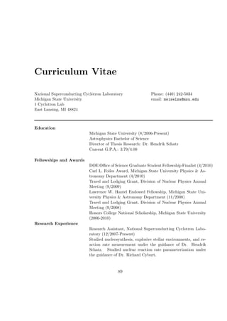
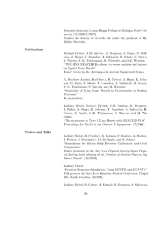


![[Illegal] gombos, justin fooling the bladder cops - the complete drug testi...](https://cdn.slidesharecdn.com/ss_thumbnails/illegalgombosjustin-foolingthebladdercops-thecompletedrugtestingguide-110806075413-phpapp02-thumbnail.jpg?width=640&height=640&fit=bounds)