A smooth-exit the-phase-transition-to-slow-roll-eternal-inflation

JHEP09(2008)036
Published by Institute of Physics Publishing for SISSA
Received: May 16, 2008
Revised: August 12, 2008
Accepted: August 12, 2008
Published: September 5, 2008
The phase transition to eternal inflation
Paolo Creminelli,a Sergei Dubovsky,bc Alberto Nicolis,d Leonardo Senatoreb and
Matias Zaldarriagabe
a
Abdus Salam International Centre for Theoretical Physics,
Strada Costiera 11, 34014 Trieste, Italy
b
Jefferson Physical Laboratory, Harvard University,
17 Oxford Street, Cambridge, MA 02138, U.S.A.
c
Institute for Nuclear Research of the Russian Academy of Sciences,
60th October Anniversary Prospect, 7a, 117312 Moscow, Russia
d
Department of Physics and ISCAP, Columbia University,
538 West 120th Street, New York, NY 10027, U.S.A.
e
Center for Astrophysics, Harvard University,
60 Garden Street, Cambridge, MA 02138, U.S.A.
E-mail: creminel@ictp.it, dubovsky@stanford.edu, nicolis@phys.columbia.edu,
senatore@physics.harvard.edu, mzaldarriaga@cfa.harvard.edu
Abstract: For slow-roll inflation we study the phase transition to the eternal regime.
Starting from a finite inflationary volume, we consider the volume of the universe at re-
heating as order parameter. We show that there exists a critical value for the classical
inflaton speed, φ̇2/H4 = 3/(2π2), where the probability distribution for the reheating
volume undergoes a sharp transition. In particular, for sub-critical inflaton speeds all dis-
tribution moments become infinite. We show that at the same transition point the system
develops a non-vanishing probability of having a strictly infinite reheating volume, while
retaining a finite probability for finite values. Our analysis represents the exact quantum
treatment of the system at lowest order in the slow-roll parameters and H2/M2
Pl.
Keywords: Cosmology of Theories beyond the SM, Spacetime Singularities, Space-Time
Symmetries.

JHEP09(2008)036
Contents
1. Introduction and setup 1
1.1 Heuristic thoughts 1
1.2 Why the system is perturbative 4
1.3 Finite comoving volume and UV smoothing 6
1.4 Space-likeness of the reheating surface 7
1.5 Quantum field vs. classical stochastic system 9
2. Volume statistics 11
2.1 The average 11
2.2 The variance 15
2.3 Uphill barrier 18
3. Bacteria model of inflation 21
3.1 Recovering the inflaton dynamics from the discrete model 23
3.2 Dead-bacteria statistics: the average 25
3.3 The variance: enhancement for the infinite line 28
3.4 Extinction probability in the semi-infinite line 31
3.5 How the probability distribution can lose its normalization 35
4. Generalization to realistic models 37
5. Summary and discussion 39
A. Proof that all moments diverge at the same Ω 41
B. Asymptotics of h1|(S + S†)m|ii 44
1. Introduction and setup
1.1 Heuristic thoughts
Consider a standard slow-roll inflationary model. At the classical level, the inflaton field φ
gently rolls down its potential, and as long as the slow-roll conditions are met the universe
inflates. Eventually, once the inflaton kinetic energy becomes comparable to the potential
energy, inflation ends and the universe reheats. At the quantum level, on top of this
classical story there are small scalar quantum fluctuations, which after re-entering the
horizon during the post-inflationary era will lead to the familiar density perturbations. In
the gauge in which the inflaton follows its unperturbed classical trajectory, δφ = 0, the
– 1 –

JHEP09(2008)036
scalar fluctuations are conveniently parameterized by the variable ζ, which measures the
spatial curvature of constant-φ hypersurfaces, (3)R = −4∇2ζ/a2. For a given inflationary
history φ(t), H(t)

the quadratic action for scalar perturbations is simply (see e.g. ref. [1])
Sζ =
Z
dtd3
x
√
−g
φ̇2
H2
1
2
∂ζ
2
, (1.1)
where the index contraction is done with the background FRW metric.
Upon canonical quantization of the above action, the typical size of quantum fluctua-
tions at horizon scales is
hζ2
iH ∼
H4
φ̇2
∼
1
ǫ
H2
M2
Pl
, (1.2)
where ǫ is the usual slow-roll parameter, ǫ ≡ φ̇2/(2H2M2
Pl). ζ then remains constant
outside the horizon, and at horizon re-entering the scalar perturbations show up as density
perturbations, with initial amplitude given by ζ itself, δρ/ρ ∼ ζ.
From a geometric viewpoint, the variable ζ is directly the dimensionless perturbation
in the spatial metric of constant-φ hypersurfaces, gij = a2(t)(1 + 2ζ) δij. Hence, small ζ
fluctuations means that these hypersurfaces are slightly curved, whereas the extreme case
of ζ of order one corresponds to a highly deformed configuration. From eq. (1.2) we see
that the latter case arises when the inflaton potential is so flat as to make φ̇2 of order H4, or
smaller. In terms of the slow-roll parameter ǫ, this happens when ǫ . H2/M2
Pl. This regime
corresponds to eternal inflation. Indeed, to see this it is convenient to switch to a different
gauge, for example a spatially flat gauge, where scalar perturbations are parametrized
through the inflaton fluctuation δφ. Then, at lowest order in slow-roll parameters, the
quadratic action is that of a minimally coupled, canonically normalized scalar in a fixed
background geometry (see for example [1]),
Sδφ =
Z
dtd3
x
√
−g
1
2
∂δφ
2
, (1.3)
whose typical quantum fluctuations at scales of order H are
h(δφ)2
iH ∼ H2
. (1.4)
On the other hand, the inflaton vev in one Hubble time advances by an amount
∆φcl = φ̇ · H−1
. (1.5)
In the ordinary, non-eternal regime quantum fluctuations are just a small correction to the
classical story. But if the classical φ̇ becomes very small — smaller than H2—the classical
inflaton advancement (1.5) drops below the typical size of quantum fluctuations. At that
point the classical downhill drift becomes unimportant and the system is dominated by
quantum diffusion. In particular backward diffusion is as likely as the forward one. Any
given observer will eventually experience reheating — because in a diffusion process the
probability for a given particle to touch any given position is always one. Nevertheless
inflation is globally eternal, in that backward diffusion, through the exponential expansion
– 2 –

JHEP09(2008)036
of the universe, leads to the creation of more and more Hubble patches which then have
a chance themselves to diffuse, and there will always be some Hubble patch that keeps
inflating. Notice that, as mentioned above, the eternal inflation regime sets in precisely
when ζ fluctuations become of order one, signaling large deformations in the geometry.
This condition was derived first in [2, 3].
The purpose of the present paper is to make progress in the quantitative understanding
of eternal inflation. Much work has been done in this direction since the first discovery
of this phenomenon [4 – 7, 2] long time ago, and some of the material, especially in this
section, will not be completely original (see two recent summaries by Guth [8] and by
Linde [9] and references therein). The main point will be to find a precise definition of
slow-roll eternal inflation (if it exists) and in particular the precise inequality that must be
satisfied by the parameters of the model to have eternal inflation.
Such a plan seems to be doomed to failure from the start. For one thing, when the
system is in or close to the eternal inflation regime, quantum fluctuations are so large as
to overcome the classical dynamics, thus impairing (a) the semiclassical approximation we
started with, and (b) the approximate homogeneity and isotropy of the universe. Once
these two features are lost, there seems to be very little hope to make any quantitative
progress. Indeed, the homogeneity issue is what usually makes so confusing the global
picture of false-vacuum eternal inflation, where bubbles of the new vacuum with different
cosmological constant keeps forming, giving rise to an intractable spacetime.
However, let’s look at these problems more closely for our slow-roll case. As to point (a)
above, large quantum fluctuations do not necessarily mean that the system is intractable.
Hardly anybody would suggest that a free scalar in Minkowski space in its vacuum state
is intractable, even though its dynamics is all in quantum fluctuations. Large quantum
fluctuations are only a problem if they are associated with strong coupling, that is if
they correspond to some interactions becoming large, thus leading to the breakdown of
perturbation theory. In other words, the issue of large fluctuations is a dynamical question
rather than a kinematical one. As long as interactions are small, a quantum field can be
reliably dealt with through the perturbative expansion. As to point (b), although in the
eternal inflation regime the typical size of ζ fluctuations at horizon scales is of order one, we
must recall that ζ parameterizes the scalar deformations in the spatial geometry induced on
the equal-φ surfaces. A large ζ means that these surfaces have a large intrinsic curvature.
This however can arise even if the four-dimensional geometry is virtually unperturbed,
but the φ fluctuations are so large as to dramatically bend the equal-φ surfaces in the
surrounding FRW geometry. In this case the full 4D geometry would still be approximately
homogeneous and isotropic, thus allowing once again for a perturbative approach.
either the full four-dimensional geometry is highly perturbed with respect to the back-
ground FRW solution, and this deformation gets projected onto the equal-φ surfaces, or
the four-dimensional geometry is virtually unperturbed, but the φ fluctuations are so large
as to dramatically bend the equal-φ surfaces in the surrounding FRW geometry. The latter
possibility is obviously harmless: in that case the full 4D geometry would still be approxi-
mately homogeneous and isotropic, thus allowing once again for a perturbative approach.
Fortunately in slow roll eternal inflation both perturbative expansions are allowed, and
are in fact one and the same, as we now explain.
– 3 –

JHEP09(2008)036
1.2 Why the system is perturbative
To see that the geometry is indeed very close to that of the unperturbed inflationary
solution, it is convenient to work in a gauge in which the metric fluctuations are mani-
festly small. This is the case for example in the gauge where the scalar perturbation is
parametrized by δφ and the equal-time hypersurfaces are flat,1
gij = a2
(t)δij . (1.6)
Then the other components of the metric at linear order are perturbed by [1]
δg00 =
φ̇
HM2
Pl
δφ ∼
√
ǫ
H
MPl
, (1.7)
δg0i = −
φ̇2
2H2M2
Pl
a2(t)
∇2
∇i
d
dt

H
φ̇
δφ

∼ a(t) ·
√
ǫ
H
MPl
, (1.8)
where we used the typical size of δφ fluctuations at horizon scales, eq. (1.4). We explicitly
see that by making ǫ smaller and smaller, we are actually suppressing the geometry fluctu-
ations [3]. In the limit of vanishing ǫ the spacetime geometry looks unperturbed, but this is
an artifact of the linear approximation. At quadratic order there are contributions to g00,
g0i of order (H/MPl)2, which dominates over the linear ones for ǫ . H2/M2
Pl—precisely in
the eternal inflation regime. Higher orders are however further suppressed by higher powers
of H2/M2
Pl, thus allowing for a perturbative expansion in such a quantity. As suggested
above, the fact that in the eternal inflation regime ζ blows up is an artifact of the strong
bending of the equal-φ surfaces in an otherwise smooth four-dimensional geometry.
Similarly, for the interactions, in the slow-roll approximation the leading interactions
come from couplings with and within the gravity sector, while the ones coming from the
potential are subdominant [1]. Then it is clear that as long as metric perturbations are
small, interactions will be small as well and the perturbative expansion will be valid.
Indeed, after integrating out the metric fluctuations (1.7), (1.8) in the same gauge as
above, one gets trilinear, two-derivative self-couplings for δφ, schematically [1]
S3 ∼
Z
φ̇
HM2
Pl
δφ ∂δφ ∂δφ . (1.9)
By using again the typical size of inflaton fluctuations, eq. (1.4), we see that at scales of
order H interactions are suppressed with respect to the quadratic Lagrangian (1.3) by
S3
Sδφ
∼
√
ǫ
H
MPl
. (1.10)
That is, for smaller and smaller ǫ the system becomes more and more perturbative. Once
again, past the critical value ǫc ∼ H2/M2
Pl new interactions start dominating, namely
1
We are restricting our analysis to scalar fluctuations. The inclusion of tensor modes is as straightforward
as uninteresting: nothing dramatic happens to them in the eternal inflation regime, their amplitude being
always of order H/MPl.
– 4 –

JHEP09(2008)036
=
~
x
t
~ dS
FRW
~
εc
ε
=
~
x
t
dS
?
ε
?
c ε 1

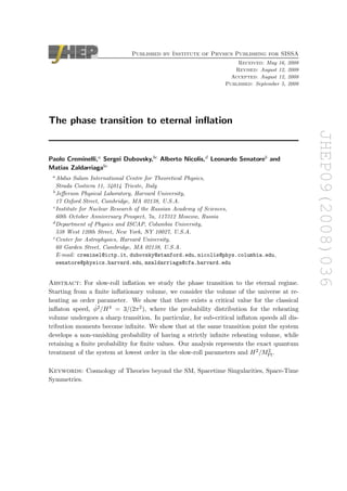
Figure 1: Left: For standard, non-eternal inflation the inflationary phase (shaded region) is nearly
de Sitter, with slow-roll corrections and small inhomogenities; the reheating surface (red curve) is
slightly bent; the post inflationary phase is nearly FRW, with small perturbations inherited from
the reheating surface. Right: In the eternal inflation regime, the inflationary phase is very well
approximated by de Sitter geometry, with corrections of order H2
/M2
Pl, but the reheating surface
has wild fluctuations; as a consequence the post-inflationary phase is highly inhomogeneous, and
intractable.
quartic, two-derivative couplings [10]
S4 ∼
Z
1
M2
Pl
∂2
δφ4
∼
H2
M2
Pl
· Sδφ , (1.11)
while higher-order interactions are suppressed by higher powers of H2/M2
Pl.
In summary, in the slow-roll regime geometry fluctuations and interactions are both
perturbative, with expansion parameters
√
ǫ · H/MPl and H2/M2
Pl in both cases. These
expansion parameters remain small even in the eternal inflation regime ζ ∼ H/(MPl
√
ǫ) ∼
1. Also for ǫ → 0 the background FRW solution tends to de Sitter space. We are therefore
led to the conclusion that in this gauge at lowest order in slow-roll and H2/M2
Pl the system
is equivalent to a minimally coupled, free scalar in a background de Sitter space, with
no dynamical gravity. In hindsight, this conclusion is obvious. In the limit in which the
potential is flat the background geometry is that of de Sitter space and the only interactions
are gravitational in nature, thus leading to effects that are suppressed by GN times the
appropriate power of the only energy scale in the problem, H. In the following we are
going to neglect all corrections in the slow-roll parameters and in H/MPl. In particular we
are going to treat as constant the slowly varying parameters H and φ̇; towards the end we
will come back to discuss what happens when this approximation is relaxed.
Of course the simplification we discussed only applies to the inflationary era. Once
inflation ends the slow-roll approximation breaks down, and ζ fluctuations get converted
into density fluctuations. For ζ ∼ 1, one gets δρ/ρ ∼ 1 when the modes come back in
– 5 –

JHEP09(2008)036
the horizon, giving rise to a highly inhomogeneous four-dimensional geometry. Therefore
in the eternal inflation regime, ζ 1, the post-inflationary era is as inhomogenous and as
confusing as the usual large-scale structure of false-vacuum eternal inflation; but as long
as we stick to the inflationary phase our picture of a free scalar in de Sitter space applies.
In any realistic inflationary scenario the breakdown of the slow-roll regime and the
consequent reheating of the universe will be gradual processes, but for our purposes it is
more convenient to picture them as instantaneously happening at some critical field value,
φ = φr. In this approximation reheating corresponds to some definite hypersurface in
spacetime. In the ordinary, non-eternal regime, φ̇/H2 ≫ 1, the spacetime region before
the reheating surface has a nearly de Sitter geometry, with small slow-roll corrections,
whereas after the reheating surface the universe is well approximated by a FRW solution
with small inhomogenities, whose amplitude is given ζ ∼ H2/φ̇. If we now make the ratio
φ̇/H2 smaller and smaller, the two above approximate descriptions tend to separate: the de
Sitter approximation before reheating becomes more and more precise up to the ultimate
accuracy of (H/MPl)2, while the FRW one after reheating becomes strongly inadequate
past φ̇/H2 ∼ 1. The situation is schematically depicted in figure 1. In the eternal inflation
regime we have no hope to quantitatively study the large-scale structure of the universe
after reheating. However, we can study the geometry of the reheating hypersurface by
approaching it from the de Sitter phase, where our approximations are well under control.
We want to sharply characterize eternal inflation through some geometric property of the
reheating surface.
1.3 Finite comoving volume and UV smoothing
A natural candidate for characterizing eternal inflation is the volume of the reheating sur-
face: if starting with a finite inflationary volume at t = 0, the reheating surface ends up
having infinite volume, we are in eternal inflation. As explained above, this should happen
below some critical value of φ̇/H2, which in our approximations is the only dimensionless
parameter of the model. Of course the volume of the reheating surface has statistical fluc-
tuations, which supposedly are very large close to the eternal inflation regime, so our goal
is to determine whether there is a sharp transition value of φ̇/H2 at which the statistical
properties of the reheating volume abruptly change.
Before studying the volume statistics, we have to define our system more precisely.
First, as we already mentioned, it is better to talk about a finite initial inflationary volume,
otherwise the reheating volume would be infinite to begin with. Let’s therefore consider
an inflationary universe compactified on a three-torus, with fixed comoving size L. L then
plays the role of an infrared cutoff for the inflaton Fourier modes. We will explicitly see
that our results do not depend on the value of L. For simplicity we will assume that at the
initial time t = 0, the size of the universe is much larger than the Hubble radius, L ≫ H−1
(we are choosing a(t) to be unity at t = 0). This is just for technical convenience, to use
integrals rather than sums in Fourier space.
Then, we want to study the constant-φ hypersurfaces, in particular that with φ = φr.
At short distances these surfaces are arbitrarily irregular, because the inflaton fluctuations
diverge at shorter and shorter scales, h(δφ)2ik ∼ k2. This leads to a UV-divergent volume
– 6 –

JHEP09(2008)036
for the equal-φ surfaces. However this is true even in Minkowski space, and it has nothing
to do with the inflationary background we are studying. We can then cutoff the high
momenta above some UV scale by smoothing out the field in space over the corresponding
UV length scale. Notice that a fixed UV cutoff in physical distances looks time-dependent
— actually exponentially shrinking — in comoving coordinates. We thus consider the
smoothed inflaton field
φΛ(~
x, t) =
Z
d3
r fΛ(r) φ(~
x + ~
r/a(t), t) , (1.12)
where fΛ(r) is a smooth function peaked at the origin and with typical width given by 1/Λ,
like for instance a Gaussian with σ = 1/Λ, and the explicit factor of a(t) gives the correct
time-dependence. Knowing the correlation functions for φ—which in the free field limit we
are working in are all determined by just the two-point function — we can compute all the
correlation functions for φΛ. In particular, φΛ too will be a Gaussian field, being a linear
superposition of Gaussian fields. It will be technically more convenient for us to work with
a sharp cutoff in momentum space and in this case we will see that our results do not
depend on the exact size of the cutoff. This strongly suggests that it does not matter how
we choose to implement the cutoff, i.e. what filter function fΛ(r) we pick. For reasons that
will soon become clear we need to smooth out the inflaton over several Hubble volumes,
that is, we need Λ−1 to be comfortably larger than H−1.
We then concentrate on the constant-φΛ surfaces. These are smooth by definition, with
no wrinkles below the UV length-scale 1/Λ. Studying these smoothed-out surfaces rather
than the original, ‘raw’ ones also makes more sense as far as reheating is concerned. Indeed,
above we were suggesting that reheating happens when the local inflaton vev reaches the
critical value φr, but of course ‘local’ has to be understood in a smoothed sense — roughly
speaking, what matters for reheating should be the inflaton average over at least one Hub-
ble volume. Once again, the fact that our results will be independent of Λ, for Λ ≪ H,
gives us confidence that the precise prescription we choose for defining the reheating surface
does not matter.
In the following we will drop the subscript ‘Λ’ from the smoothed field φΛ, and the
smoothing will be understood unless otherwise stated.
1.4 Space-likeness of the reheating surface
Our smoothing procedure is also important for making the reheating surface space-like.
Indeed, when we talk about computing the volume of the reheating surface, we are im-
plicitly assuming that such a surface is space-like, so that its volume can be interpreted
as the volume of the universe at the end of inflation. If such a surface were not space-
like everywhere, the ‘end of inflation’ would not be an event in time, but rather in some
space-time region it would look like a boundary in space. Also, the induced metric on
the surface would not be positive-definite everywhere. The space-likeness of the reheating
surface is not obvious when quantum fluctuations are taken into account. In the classical
limit the reheating surface is obviously space-like, as the classical motion gives a φ̇ with
definite sign. Quantum corrections add an additional motion to the classical one, as more
– 7 –

JHEP09(2008)036
and more modes enter in the filter fΛ(r) of eq. (1.12). It is not obvious that the resulting
motion gives rise to a space-like reheating surface.2
Fortunately the smoothing procedure helps in this respect: the probability for a
constant-φ surface not to be space-like somewhere is suppressed by ∼ e−H2/Λ2
, where
Λ ≪ H is our UV cutoff. To see this, consider the inflaton field φ, without any smoothing
filter. The equal-φ surfaces are space-like if and only if φ itself is a good time variable, that
is if and only if ∂µφ is time-like everywhere,
(∂φ)2
0 (1.13)
(we use the (+, −, −, −) metric signature). Of course φ is a quantum field, and the above
condition cannot hold as an exact operator statement: at any space-time location there is
always a finite probability for ∂µφ to point in a space-like direction. The best we can hope
for is to make the above inequality valid as an expectation value, and quantum fluctuations
around it small; this issue is general, and it is not peculiar to the eternal regime we want to
study. As to the expectation value, if we split the field into background plus fluctuations,
we have
h(∂φ)2
i = φ̇2
+ h(∂δφ)2
i , (1.14)
where φ̇ is the classical inflaton speed, and δφ in our approximations is well described by
a free, minimally coupled scalar in de Sitter space. The fluctuating piece h(∂δφ)2i is UV
divergent; if we cut it off at some physical momentum Λ we get
h(∂δφ)2
i = −
Z Λ·a(t)
d3k
(2π)3
1
a2(t)
H2
2k
= −
H2
8π2
Λ2
, (1.15)
which is negative. We thus see that quantum fluctuations tend to violate eq. (1.13), and
that the equal-φ surfaces cannot be assumed to be space-like at arbitrarily short scales.
Only for length-scales larger than the critical UV cutoff
Λ−1
c ∼
H
φ̇
= H−1
·
H2
φ̇
(1.16)
does the classical piece in eq. (1.14) dominate over the quantum one. We stress again
that this conclusion also applies to standard, non-eternal inflation. For instance, at scales
shorter than the above critical cutoff there is no sense in which one can use φ itself as
a clock and define the equal-time surfaces by the gauge-fixing δφ = 0. Notice however
that in the non-eternal regime φ̇/H2 is much larger than one and so the critical cutoff is
parametrically smaller than the Hubble radius; on the other hand close to or in the eternal
regime φ̇/H2 is of order one, thus making the critical cutoff of order of the Hubble radius.
2
For a generic inflaton value, different from the reheating one, it is not even clear whether it makes sense
to talk about ‘surface of constant inflaton value’. Taking into account quantum fluctuations in the direction
opposite to the classical motion, it is possible to go through the same value of the inflaton many times, so
that the points of constant inflaton value will not form a smooth manifold. This cannot happen for the
reheating surface, because by definition after crossing φr inflation ends and the system cannot fluctuate
back again.
– 8 –

JHEP09(2008)036
This is why in our smoothing procedure we choose to filter out all modes with wavelengths
smaller than Λ−1 ≫ H−1.
Similarly for the standard deviation of eq. (1.13), at scales larger than 1/Λc the dom-
inant contribution comes from cross-product terms,
q

(∂φ)2 − h(∂φ)2i
2
∼
q
φ̇2 h(δφ̇)2i ∼ φ̇ · Λ2
, (1.17)
Requiring this to be negligible compared to the classical value φ̇ gives a constraint on Λ:
Λ Λc ≃ φ̇1/2, which is stronger than (1.16). In the eternal inflation regime however,
φ̇ ∼ H2, so that this just reiterates the conclusion that the cutoff must be parametrically
smaller than H.3
In summary, if we smooth out the inflaton field over length-scales somewhat larger than
the Hubble radius, we can safely assume that the constant-φ hypersurfaces are space-like.4
Of course there is always a non-vanishing probability of having a large quantum fluctuation
that locally brings ∂µφ onto a space-like direction. However thanks to the gaussianity of
the inflaton fluctuations, such probability is exponentially small with a width given by
eq. (1.17), roughly
P (∂φ)2
0

∼ e
− φ̇2
φ̇Λ2
∼ e−H2/Λ2
. (1.18)
We stress again that the same arguments hold in the non-eternal regime: the gauge fixing
δφ = 0 only make sense with a sufficiently small cutoff Λ and neglecting exponentially
small corrections similar to the equation above.
1.5 Quantum field vs. classical stochastic system
Another reason why we need Λ−1 ≫ H−1 is that, in this approximation, as it was already
noticed in the context of eternal inflation in [2, 11], we can neglect the quantum nature
of the field and treat it as a classical stochastic system. Consider a single Fourier mode
of the scalar field; as we are neglecting interactions, it simply behaves as an harmonic
oscillator with parameters that depend on the background and are thus time dependent.
As it is well known, in the limit in which the mode wavelength is much larger than the
Hubble scale, the system is in a squeezed state with very large squeezing parameter [17].
3
Eq. (1.17) is the correct expression in the eternal case, where we must choose Λ ≪ H. In the non-eternal
case, if we allow for Λ ≫ H there is another competing term of the form Λ4
. Anyway one ends up with the
constraint Λ Λc ≃ φ̇1/2
which is parametrically shorter than the Hubble radius in the non-eternal regime.
4
One may argue that, although the smoothed reheating surface is spacelike, the real one may be not,
as reheating will be sensitive to scales of order H−1
and not much larger. This would be problematic at it
implies the existence of inflating points in the future light-cone of points where inflation already finished. As
we discussed, the post-inflationary era is not under control and it would therefore be impossible to proceed.
However, a model in which a potential giving eternal inflation abruptly ends and reheats is an idealization.
One should consider a realistic potential where ζ ≪ 1 close to reheating. As we will discuss later, this
period of non-eternal inflation does not change our conclusions, but it introduces a physical smoothing of
the reheating surface, as at short scales ζ is very small. This implies that the reheating surface is space-like.
This is the most physical way of looking at our smoothing procedure: the effect of a final period of inflation
during which quantum fluctuations are small. We thank Ben Freivogel and Raman Sundrum for discussions
about this point.
– 9 –

JHEP09(2008)036
This corresponds to the fact that the dynamics is dominated by the so called “growing
mode”, while the other independent solution dies away exponentially (“decaying mode”).
Although the system is still fully quantum, we expect that all physical measurements and
interactions will only be sensitive to the growing mode so that the decaying one can be
disregarded. This leads to a classical system, with the amplitude of the growing mode as
a classical stochastic variable.5
In conclusion, under our approximations the inflaton fluctuations are well described
by a classical stochastic field with Gaussian statistics. All correlation functions are then
determined uniquely by the two-point function. At equal times, before smoothing this is
hδφ(~
x, t) δφ(~
y, t)i =
1
(2π)2
1
|~
x − ~
y|2 a2(t)
−
H2
(2π)2
log
|~
x − ~
y|
L
, (1.19)
where L is our IR cutoff — the comoving size of the universe. The first term is the usual
two-point function for a massless scalar in Minkowski space. The second piece is peculiar
to de Sitter space, and it is the celebrated scale-invariant spectrum. Upon smoothing out
the field, the above expression is the correct one at distances larger than the UV cutoff,
|~
x − ~
y| · eHt ≫ Λ−1, whereas at shorter distances the two points can be thought of as
coincident and we get the classic result [12 – 14]
h(δφ2
(~
x, t))i = αΛ2
+
H2
(2π)2
log ΛL + β + Ht

=
H3
(2π)2
t + const . (1.20)
As usual, the coefficient of the quadratically divergent piece, α, as well as the finite part
associated to the log-divergent piece, β, are order-one numbers that are regularization-
dependent, i.e. they depend on the precise filter-function we adopt to smooth-out the
field. On the other hand, the coefficient in front of the log-divergence is regularization-
independent, being determined by long-distance physics. The factor of t comes from the
explicit time-dependence of the UV-cutoff in comoving coordinates, or, equivalently, from
the time-dependence of the IR cutoff in physical coordinates. Physically, as time goes on
more and more modes are included in the smoothed field and, given the scale-invariance
of the spectrum, they all contribute to the variance (1.20). The coefficient of t is also
regularization-independent, being determined by the log-divergence coefficient and by how
the cutoff scales with time — not by the precise definition of the cutoff.
We see that the variance of δφ at a given comoving point ~
x increases linearly with time.
This reminds us of a random walk and it is the base of the so called stochastic approach
to inflation which dates back to [15, 2, 11]. Indeed, if as smoothing procedure we choose
a sharp cutoff in momentum space, the analogy becomes exact: at any given point δφ(~
x)
undergoes a random walk, every new mode included in the smoothing giving a random
kick to the field, totally uncorrelated to the previous ones. This will allow us to exploit
the technology of diffusion processes.
5
Referring to the discussion of footnote 4, we can again assume that a period of non-eternal inflation,
ζ ≪ 1, stretches all the relevant modes largely out of the horizon, so that we are indeed allowed to treat
them classically.
– 10 –

JHEP09(2008)036
Before moving to the actual calculations, we want to underline the simplicity of the
system under study. Everything has been reduced to a free scalar in de Sitter space. Going
towards the eternal inflation regime however, we will see that this system gives rise to a
kind of phase transition producing an infinite reheating volume. Although we are studying
a free field, the relation between the reheating volume and the scalar is very non-linear and
this is what gives rise to the interesting dynamics.
2. Volume statistics
2.1 The average
Let us study the probability density ρ(V ) for the volume of the reheating surface φ = φr.
Our goal is to identify a sharp transition in the behavior of this probability density at
some finite value of the parameters of the model. In the setup discussed in the previous
section the only dimensionless parameter is given by the quantity φ̇/H2, the ratio between
the classical motion and quantum fluctuations. We want to see whether it is possible to
identify a critical value of φ̇/H2 where a sharp transition in the properties of ρ(V ) occurs.
This would correspond to the onset of the eternal inflation regime.
Let us start with calculating the average reheating volume hV i
hV i =
Z
dV V ρ(V ) . (2.1)
If we call tr(~
x) the reheating time as a function of the comoving coordinate ~
x, the average
volume can be written as
hV i =

Z
d3
x e3Htr(~
x)

=
Z
d3
x

e3Htr(~
x)

, (2.2)
where we reversed the order of integration and averaging thanks to linearity of both. Then
the problem becomes very simple:
hV i = L3
Z
dt e3Ht
pr(t) , (2.3)
where pr(t) is the probability that at a given point ~
x the field reaches the reheating value
φr at time t. By translational invariance this probability does not depend on the point ~
x,
so that the integral over the comoving coordinates can be factored out to give the volume
of the comoving box L3.
To obtain the probability of reheating at time t we have to start from the probability
P(φ, t) of having a given field value φ at time t. This again does not depend on the point
~
x. Then the probability to reheat at time t can be calculated as time-variation of the
probability of still being inflating, i.e. of having φ anywhere on the left of φr:
pr(t) = −
d
dt
Z φr
−∞
dφ P(φ, t) . (2.4)
As we already discussed in the previous section, at leading order in the slow roll parameters,
the perturbation of the inflaton field around the classical slow roll solution,
ψ = φ − φ̇t (2.5)
– 11 –

JHEP09(2008)036
tr
t
Φ
tr
t
Ψ
Figure 2: At any given comoving point, the local inflaton value undergoes a random walk. Left:
for φ the reheating barrier is held fixed at φ = φr, but there is classical drift towards it. Right: for
the fluctuation ψ there is no net drift, but the barrier is approaching at a speed φ̇.
is a Gaussian field with variance σ2 that grows linearly with time (see figure 2),
σ2
=
H3
4π2
t . (2.6)
Here we dropped t-independent terms present in the full expression (1.20). It is straight-
forward to keep track of these terms and check that they do not affect our results, that
depend only on the late time asymptotics of σ2. In fact the constant pieces in eq. (1.20)
can be set to zero by a constant shift of the time variable, t → t + const. All properties of
the system that are dominated by the t → ∞ limit — like whether inflation is eternal or
not — are totally insensitive to such a shift. Note that the UV cutoff Λ does not enter in
the t-dependent part (2.6), nor does the IR cutoff L, so that our conclusions are not sensi-
tive to the values of Λ and L. To avoid the proliferation of numerical coefficients, in what
follows it is convenient to use σ2 itself as time variable. At any given ~
x, the probability
distribution P(φ, t), when written as a function of ψ and σ2, satisfies the diffusion equation
∂P
∂σ2
=
1
2
∂2P
∂ψ2
. (2.7)
Inflation ends when the inflaton field φ reaches φr. Consequently, we are interested in
solving the diffusion equation (2.7) with an “absorbing barrier” at the corresponding value
of ψ, i.e. the solution should satisfy the Dirichlet boundary condition
P|ψ=ψr = 0 , (2.8)
with
ψr = φr − φ̇t = φr − 4π2 φ̇
H3
σ2
. (2.9)
Such a solution can be constructed by using a generalization of the method of images. One
starts with the standard solution describing diffusion without any barriers and with initial
condition localized at ψ = 0 for t = 0
P0(ψ, σ2
) =
1
√
2πσ2
e−ψ2/2σ2
. (2.10)
– 12 –

JHEP09(2008)036
In the case of a time independent barrier, it is well known that the Dirichlet boundary
condition can be satisfied adding a negative image located specularly with respect to the
barrier. In our case we have a barrier moving linearly in time. It is straightforward to
show that in this case the solution becomes
P1(ψ, σ2
) =
1
√
2πσ2

e−ψ2/2σ2
− e8π2φ̇ φr/H3
e−(ψ−2φr)2/2σ2

. (2.11)
The image is symmetric with respect to the barrier position at time t = 0 and it is multiplied
by a constant factor which depends on the barrier speed. Note that in the whole physical
region, ψ ψr, the contribution from the image is smaller than the P0 term, as it should
be in order for the density distribution P1 to remain positive. Far from the barrier the
contribution of the image is exponentially suppressed.
We can now use our solution for P to evaluate the probability (2.4) of reheating at a
given time t. By making use of the diffusion equation (2.7) and taking into account that
P vanishes on the barrier, eq. (2.8), we have
pr(t) = −
H3
8π2
∂P
∂φ

ψ=φr−φ̇t
. (2.12)
Disregarding the polynomial dependence in front of the exponential we have
pr(t) ∼ e−2π2 (φr−φ̇t)2
H3t . (2.13)
At late times this gives for the volume (2.3)
hV i ≃ L3
Z ∞
0
dt α(t) e3Ht− 2π2 φ̇2
H3 t+O(1)
, (2.14)
where the prefactor α(t) does not have exponential dependence on time. We see that the
average reheating volume remains finite if and only if
Ω ≡
2π2
3
φ̇2
H4
1 . (2.15)
So far we have not talked about the initial condition we choose for the inflaton. Clearly, as
the general solution of the diffusion equation is given by the convolution of P1(ψ, t) with
the initial probability distribution, the initial condition is irrelevant for the convergence
of the average reheating volume. A similar criterium for the divergence of the inflating
volume was put forward in [16]. Here we focus on the more physical quantity of reheating
volume and we proceed to better characterize what happens at Ω = 1.
Equation (2.15) appears as a sharp criterion for whether eternal inflation takes place
or not. At the end we will argue that this is essentially correct; however to justify this
conclusion we first need to address several important subtle points. Let us try to understand
in more detail what happens to the probability distribution for the reheating volume ρ(V )
at the critical value Ω = 1, where the average reheating volume diverges. There are two
possible options. First, it may happen that each moment hV ni of the distribution has a
– 13 –

JHEP09(2008)036
different critical value of Ω when it starts diverging. This would happen, for instance, if
ρ(V ) had a power law asymptotics at large values of V with the power depending on Ω, e.g.
ρ(V ) ∝
1
1 + V 1+Ω
. (2.16)
If this were the case, the value Ω = 1 associated to the divergence of hV i would not re-
ally mark any sharp transition in the physical behavior. Each moment of the distribution
would single out a different transition point. Perhaps in this case a better characterization
of the onset of eternal inflation would be given by the value of Ω where the probability
distribution itself ceases to be normalizable (Ω = 0 for the model distribution (2.16)), if
such a value exists.
The other possibility is that at Ω = 1 all moments of the probability distribution
becomes infinite, including the “zeroth” moment, i.e. the probability distribution also ceases
to be normalizable at this point. This would happen, for instance, for a family of probability
distributions of the form
ρ(V ) ∝ q(V )e(1−Ω)V
, (2.17)
where q(V ) has a power-law behavior at large V . In this case the critical value Ω = 1
indeed has a very sharp physical meaning.
We will see that the actual answer is somewhat more complicated than both of these
options. However, already at this point it is possible to argue that in the setup we are
considering the distribution is not of the type (2.17) and that different moments diverge
at different values of Ω. Indeed, it is straightforward to see that for any given value of Ω
there is a value n0 such that all moments of the volume distribution hV ni with n n0
diverge. Indeed, let us imagine that Ω is much larger than one, so that naively one is very
far from the eternal inflation regime. Let us consider a class of inflaton trajectories that
at time t in one Hubble patch have a huge quantum fluctuation in the direction opposite
to the classical motion, such that the inflaton ends at
φ = φr − φ̇t . (2.18)
The classical trajectory would have φ = φ̇t, so that at large t the probability of such a
fluctuation is exponentially suppressed by a factor of order e−A·Ht, with A ∼ φ̇2/H4 ∼
Ω2. The important point is that the exponent grows only linearly with time (and not
quadratically). The reason is that the variance σ2 of the inflaton perturbation ψ is itself
a linear function of t. Then, with probability close to one such a trajectory will give rise
to a reheated volume at least as big as e3HtH−3, since this is the volume one would get
just classically rolling down from φ = φr − φ̇t to φ = φr. Consequently, for n A/3 ∼ Ω2
the contribution to the moment hV ni from this set of trajectories grows exponentially as a
function of t—the large power of the exponentially growing volume over-compensates for
the small probability of the required fluctuation — and these moments diverge.
At this point one is tempted to conclude that the situation is analogous to what
happens with the distribution (2.16) and that there is no sharp transition to the eternal
inflation regime. We will argue later that this conclusion is too quick, and that instead
– 14 –

JHEP09(2008)036
there is a sharp transition. Notice that for the rough argument about higher moments to
work, it is essential to consider, as time grows, backward fluctuations that go further and
further along the potential without bound. To see what this implies, it is instructive to
understand the effect we just described at a more quantitative and detailed level. For this
purpose we are going to study now the behavior of hV 2i and show that indeed it starts
diverging at a critical value Ω 1, i.e. when the average volume hV i is still finite.
2.2 The variance
The calculation we did for the average is deceivingly simple as the only thing we needed
was the 1-point probability P(φ, t) to have a value of the field φ at time t, which is clearly
independent of the comoving position ~
x. However the study of the full probability for the
reheating volume ρ(V ) is not straightforward as the only expression for it is based on a
functional integration over the field realizations
ρ(V ) =
Z
Dφ P[φ] δ V −
R
d3x e3Htr(~
x)

, (2.19)
where Dφ is the functional measure on the set of all possible space-time realizations of the
inflaton field, P[φ] is the probability of a specific realization and tr(~
x) is the reheating time
for a given realization as a function of the comoving coordinate ~
x.
Instead of trying to evaluate the expression above, to calculate hV 2i we will follow
a procedure similar to the one used for the average. Namely, let us define the 2-point
probability distribution of the inflaton field P2(φ1, φ2, |~
x1 − ~
x2|, t1, t2), such that
P2 dφ1dφ2 (2.20)
gives the joint probability of finding the inflaton field in the ranges (φ1(2), φ1(2) + dφ1(2)) at
the two space-time points (~
x1, t1) and (~
x2, t2). For translational and rotational invariance
this joint probability just depends on the distance between the two points |~
x1 − ~
x2|. Anal-
ogously to the previous section we can define a probability density p2r(t1, t2, |~
x1 − ~
x2|) for
reheating to happen at the comoving point ~
x1 at time t1 and at the comoving point ~
x2 at
time t2. Similarly to (2.4) this will be related to P2 by
p2r(t1, t2, |~
x1 − ~
x2|) = −∂t1 ∂t2
Z φr
−∞
dφ1
Z φr
−∞
dφ2 P2(φ1, φ2, |~
x1 − ~
x2|, t1, t2) . (2.21)
Then the expectation value of V 2 can be written as
hV 2
i =
Z
d3
x d3
y e3Htr(~
x)
e3Htr(~
y)

= L3
Z
dt1dt2d3
x e3Ht1
e3Ht2
p2r(t1, t2, |~
x|) . (2.22)
To study the convergence of this integral we need to find the 2-point probability P2.
For fixed comoving distance |~
x| between the two points this probability has a very different
behaviour at early and late times. At early times,
t1, t2 ≪ t∗ ≡ −H−1
log H|~
x| , (2.23)
– 15 –

JHEP09(2008)036
t* tr1 tr2
t
Φr
Ψ
Figure 3: Our two-step approximation. The local inflaton fluctuations in two nearby comoving
points are assumed to be totally correlated until the physical distance between the two points exits
the UV cutoff (t t∗), and totally uncorrelated afterwards (t t∗).
the two points are within one Hubble patch and therefore they are not resolved by the
smoothing procedure. As such their evolution is perfectly correlated. In particular the
2-point distribution at equal times t1 = t2 is just given by the 1-point distribution (2.11),
P2(ψ1, ψ2, |~
x|, t, t) ≃ P1(ψ1, t)δ(ψ1 − ψ2) for t ≪ t∗(|~
x|) . (2.24)
In the opposite limit, when the distance is much larger than the Hubble radius, the inflaton
fluctuations at the two points are completely uncorrelated. In this case, the probability
distribution P2 satisfies a diffusion equation with respect to each pair of variables (t1, φ1),
(t2, φ2),
∂P
∂σ2
1(2)
=
1
2
∂2P
∂ψ2
1(2)
for t1, t2 ≫ t∗ . (2.25)
In the equations above ψ1(2) and σ2
1(2) are related to t1(2) and φ1(2) by the relations (2.5)
and (2.6).
In the following we are going to use a “two steps” approximation in which we consider
a single random walk before t∗ and two uncorrelated ones after t∗, as dipicted in figure 3.6
The exact solution is more complicated as there is an intermediate period of partial corre-
lation [18]. However it will be easy to check that our results will not depend on the exact
definition of t∗, when the two regimes are matched. This strongly indicates that taking
into account the period of partial correlation would not change the range of Ω when hV 2i
converges.
In this 2-step approximation, the 2-point probability when the distance between the
two points is larger than Hubble is obtained first following a single random walk until the
6
The same approximation has been used in the study of structure formation in [18].
– 16 –

JHEP09(2008)036
time of “separation” t∗ and then convolving this initial condition with two independent
Green’s functions for the diffusion equation with a barrier. This translates into
P2(ψ1, ψ2, |~
x|, t1, t2) =
Z φr−φ̇t∗
−∞
dψ G(ψ1, ψ, t1 − t∗)G(ψ2, ψ, t2 − t∗)P1(ψ, t∗) , (2.26)
with t1, t2 t∗. Notice that the dependence on |~
x| is hidden in t∗, given by equation (2.23).
The Green’s function G is straightforward to construct by making use of the solution (2.11).
Namely, it is equal to
G(ψ1, ψ, t) = P̃1(ψ1 − ψ, t − t∗) (2.27)
where “tilde” indicates that φr in eq. (2.11) must be replaced by
φr − ψ − φ̇t∗ (2.28)
to take into account that the independent motion of each of the two points starts at ψ at
time t∗, rather than at the origin at t = 0.
To prove that the variance diverges when the average volume is still finite, it is enough
to obtain a lower bound on the integral (2.22). As the integrand is positive definite, we
can therefore restrict the range of integration by considering only pairs of points (~
x1, ~
x2)
in different Hubble patches (both at t1 and at t2). In other words we can impose a UV
cutoff on the integration over the comoving volume in eq. (2.22) by requiring
t∗(|~
x|) t1, t2 . (2.29)
It is anyway straightforward to check that the remaining range of integration gives a con-
tribution that always converges whenever Ω 1.
As before we can use (2.25) to evaluate the integrals in (2.21) and arrive at the following
expression
hV 2
i=−
H6 · L3
64π4
Z ∞
0
dt1dt2
Z
|~
x|H−1e−Hτ
d3
x e3H(t1+t2)
∂ψ1 ∂ψ2 P2(ψ1, ψ2, |~
x|, t1, t2)

ψ1(2)=φr−φ̇t1(2)
,
(2.30)
where τ = min(t1, t2).
The partial derivatives act on each of the two Green functions of eq. (2.26) and give
a dependence analogous to the 1-point case eq. (2.13). The evolution before splitting
given by P1 contains the image term and one should sum the two contributions. However,
as already discussed in the previous section, we will find that the divergence of hV 2i is
dominated by trajectories which are exponentially far from the barrier as time becomes
large. This implies a posteriori that the image term is completely irrelevant.
The convolution integral in (2.26) can be done in saddle point approximation. The
saddle point is given by
ψsaddle = t∗
(ψ1 + ψ2) t∗ − t2ψ1 − t1ψ2
t2
∗ − t1t2
. (2.31)
This gives for the exponential part of P2
P2(ψ1, ψ2, |~
x|, t1, t2) ∼ exp

−
2π2
H3
·
t2ψ2
1 − 2t∗ψ1ψ2 + t1ψ2
2
t1t2 − t2
∗

. (2.32)
– 17 –

JHEP09(2008)036
Note that this expression non-trivially depends on the spatial separation |~
x| through the
horizon crossing time t∗, as shown in (2.23). To plug this result back in (2.30) it is conve-
nient to use
t± = t1 ± t2 (2.33)
as time variables and the horizon exit time t∗(|~
x|) in place of the comoving separation ~
x.
With this change of variable and keeping only the leading exponential behavior at large
times as in the previous section, one obtains (restricting to t1 ≥ t2)
hV 2
i ∼
Z ∞
0
dt+ e3Ht+
Z t+
0
dt−
Z t+−t−
2
0
dt∗ e−f(t+,t−,t∗)
, (2.34)
where
f(t+, t−, t∗) = 3Ht∗ + 3HΩ

t+ − 2t∗ +
4t2
∗(t+ − 2t∗)
t2
+ − t2
− − 4t2
∗

. (2.35)
The first term on the right hand side of this equation comes from the change of integration
measure from x to t∗(|~
x|). To check whether the integral over t+ converges, we can minimize
the function f with respect to t− and t∗ in the range of integration. As t− enters into f
only in the denominator of the last term, it is clear that the saddle point is
t− = 0 . (2.36)
Then the minimization with respect to t∗ gives
t∗min =
t+
2
√
2Ω − 1

, (2.37)
and the value of f at this minimum is
f(t+, 0, t∗min) = 3Ht+

√
2Ω −
1
2

. (2.38)
This grows faster than 3Ht+ for
Ω
9
8
. (2.39)
We conclude that hV 2i ceases to be finite when the parameter Ω drops below 9/8, i.e. before
the average volume hV i starts diverging. As a consistency check of the calculation, note
that at Ω = 9/8 the optimal horizon exit time t∗min indeed belongs to the integration
interval in (2.34). For Ω 2 this would no longer be true and the dominant contribution
would come from t∗ = t+/2: hV 2i would be dominated by the dynamics before the two
points become independent.
2.3 Uphill barrier
The above explicit calculation of hV 2i nicely fits into the general argument presented at
the end of section 2.1. We have seen that, in saddle point approximation, the dominant
contribution to hV 2i comes from points that reheat at the same time t1 = t2. These points
start evolving independently when separated by a physical distance ∼ H−1; this happens
– 18 –

JHEP09(2008)036
at a fraction of the eventual reheating time, which is equal to 1/2 for the critical value
Ω = 9/8, see (2.37).
Where is the most likely position along the potential at t∗, when the two points start
their independent evolution? From the saddle point result (2.31) we see that it is a position
with a huge backward fluctuation with respect to the classical trajectory
ψ = −
r
2
Ω
φ̇ t∗min . (2.40)
For Ω 2 this fluctuation corresponds to a negative value of the inflaton
φ =

1 −
p
2/Ω

· φ̇t∗min , (2.41)
so that the most likely position at t∗min is higher than the starting point at t = 0 and it
becomes higher and higher without bound for t∗min → ∞. This agrees with the general
argument above.7
To summarize, all this sounds as if the volume distribution has qualitative properties
similar to the model distribution (2.16), where the various moments start diverging at dif-
ferent values of Ω. Thus it seems that the value Ω = 1, where the average volume diverges,
does not really correspond to any sharp physical transition. However this conclusion is too
quick. In section 3, where we study a discretized version of the same system, we will argue
that at Ω = 1 another sharp transition occurs besides the divergence of hV i: the total
probability of having a finite reheating volume becomes smaller than one! This property
is expected in the transition into the eternal inflation regime as it tells us that there is a
finite probability of an infinite reheating volume or equivalently for inflation to last for-
ever. Clearly this sharply defines Ω = 1 as the transition point to eternal inflation. Before
moving to this issue, let us conclude our study of the moments of the distribution ρ(V ).
As we stressed, the divergence of the higher moments is qualitatively different with
respect to the case of the average. The explicit calculation of hV 2i, following the general
argument made in section 2.1, shows that the divergence is related to the possibility of
fluctuating uphill without bound, infinitely far from the barrier. What we are going to
check is that, if we put a bound to the possibility of going infinitely uphill, all the moments
diverge at the same critical value Ω = 1.
To impose a limit on fluctuations infinitely far from the reheating point, we can put a
reflecting barrier so that the field value is constrained to satisfy
φ φup , (2.42)
where φup will be a large negative value. The value of ψ at the barrier will be given by
ψup = φup − φ̇t . (2.43)
Here we are going to study the effect of this new barrier on the calculation of hV 2i,
while we postpone the discussion about all higher moments to appendix A. We do not
7
Notice that as hV 2
i is dominated by a splitting point infinitely far away from the barrier it is justified
disregarding the image terms of the probability P1 in (2.26).
– 19 –

JHEP09(2008)036
need to find the explicit form of the solution of the diffusion equation with two barriers.
To keep track of the late time exponential behavior for large enough |φup|, it is enough to
consider that the integration range in the convolution (2.26) is now restricted to (ψup, ψr)
and it is not extended infinitely uphill. For Ω 2 the saddle point position (2.41) moves
backwards and thus it eventually hits the new uphill barrier. The saddle point exits the
physical region and therefore, in the leading exponential approximation, the result will be
dominated by a splitting point position on the uphill barrier, i.e. the point closest to the
(would-be) saddle. In this approximation one obtains for the 2-point distribution
P2(ψ1, ψ2, |~
x|, t1, t2) ≃ exp

−
2π2
H3
(ψ1 − ψup)2
t1 − t∗
+
(ψ2 − ψup)2
t2 − t∗
+
ψ2
up
t∗
!#
. (2.44)
We are interested in the late time behaviour of this expression. The position of the uphill
barrier φup becomes irrelevant in this limit as it is dominated in (2.43) by the time de-
pendent term. This means that φup disappears from the calculations and therefore from
the final critical value of Ω and it can be thought just as a regulating device, which can
be sent to infinity. Notice however that its effect is crucial. Mathematically this comes
from the fact that the large φup limit and the late time limit do not commute, because
the saddle point (2.31) eventually exits the integration region at any finite value of φup.
In more physical terms this means that no matter how far the barrier is there will be a
sufficient large time such that
H3
t φ2
up (2.45)
so that the diffusion is so large to be sensitive to the presence of the extra barrier. As
the transition to eternal inflation is sensitive to arbitrarily large times, the presence of the
regulating barrier will be important, independently on how far we put it.
To see that the presence of the second barrier changes the value at which hV 2i diverges,
let us plug (2.44) in the expression (2.30) for the hV 2i. We obtain the same result as (2.34)
with the function f now taking the form
f(t+, t−, t∗) = 3Ht∗ + 3HΩ (t+ − t∗) (2.46)
We see that now the integral for hV 2i converges for Ω 1. Note that the integral over t∗
is saturated at the upper limit, justifying a posteriori an assumption implicit in the whole
derivation — that in the late time limit (meaning large t1,2 limit) t∗ also indefinitely grows.
On the other hand it is easy to check that there is no effect of the second barrier on
the calculation of hV i; this is just a consequence of the fact that solutions to the diffusion
equation behave continuously when one removes one of the barriers to infinity. This is
checked in appendix A, where we study the explicit solution in the presence of two barriers.
In conclusion, in the presence of an uphill regulating barrier, Ω = 1 is the critical point
both for hV i and for hV 2i. In appendix A we will see that this holds also for all higher
moments hV ni.
– 20 –

JHEP09(2008)036
i+1 1 0
p
1−p
i i−1
Figure 4: The branching process.
3. Bacteria model of inflation
The above results strongly suggest that Ω = 1 sets the transition to eternal inflation. To
conclusively confirm this one would like to directly check that at Ω 1 there is a finite
probability for inflation to run forever. A natural quantity to look at to address this issue
is the total probability to have a finite reheating volume,
Pf =
Z
dV ρ(V ) , (3.1)
where ρ(V ) is the volume probability distribution defined by eq. (2.19). Clearly, Pf = 1 if
inflation always ends in a finite time. On the other hand, as we will see in this section, for
Ω 1 the total probability Pf drops below one. This is a direct signal of eternal inflation
— in this regime there is a finite probability (1−Pf ) that the total volume of the reheating
surface is infinite. This result also shows that the transition to the eternal regime is quite
similar to a second order phase transition, with (1 − Pf ) being an order parameter.
To derive this result one needs more detailed information about the probability distri-
bution ρ(V ) rather than just its multipole moments. This seems to be hard to achieve, as
the only available definition of ρ(V ) is a rather formal functional integral formulae (2.19).
As usual with functional integrals, to gain more control over ρ(V ) it is natural to switch
to a discretized description of the inflationary dynamics. This will be the approach of the
current section.
With a biological analogy, consider at t = 0 a bacterium that can live in a discrete set
of positions along a line (see figure 4). At t = 1 the bacterium splits into N copies. Then,
each bacterium (independently of all the others) hops with probability p to the neighboring
site on its right, and with probability (1 − p) on the left. N and p are fixed numbers. At
t = 2 each second-generation bacterium reproduces itself, and so on. The analogy with our
inflationary system is clear: each bacterium represents an Hubble patch; sites are inflaton
values. Reproduction is the analogue of the Hubble expansion; at every e-folding ∼ e3 new
Hubble volumes are produced starting from one. From then on the inflaton inside each
Hubble volume evolves independently, with a combination of classical rolling and quantum
diffusion. This is represented by the random hopping of our bacteria. The difference in the
probabilities of moving right and left gives a net drift, and thus corresponds to the classical
motion. To complete the analogy we have to assume that there is a “reheating” site, i = 0
in the figure: when a bacterium ends up there it stops reproducing and moving around — it
dies. In the previous sections we studied the statistical properties of the reheating volume
– 21 –

JHEP09(2008)036
V as a function of Ω. In the bacteriological analogy the reheating volume corresponds to
the number of dead bacteria (= non-reproducing Hubble patches) in the asymptotic future.
For analogy we denote the latter quantity by V , which of course now takes discrete values.
Our task is to study the probability distribution of V as a function of the parameter p.
A discrete system like the one we described goes under name of branching process, more
precisely a multi-type Galton-Watson process (see e.g. ref. [19]). Similar models have been
studied in the context of eternal inflation in [20]. Here the focus will be the relationship with
the continuum case and the precise characterization of what happens at the critical point.
Before moving to the explicit study of the model, let’s summarize the main results we
will achieve:
• We will explicitly show that in a suitable continuum limit the discrete model precisely
converges to the full inflationary case we studied in the previous sections.
• There is a critical value pc 1/2 such that for p ≤ pc the expectation value hV i of the
number of dead bacteria at future infinity diverges, whereas it converges for larger
p’s. For inflation, pc is the analogue of the critical Ω below which the expectation
value of the reheating volume becomes infinite. We shall see that in the continuum
limit the value of the critical Ω that we can infer from the discrete model matches
the one obtained directly in the inflationary case.
• The behavior of the variance of V crucially depends on whether we consider a semi-
infinite or finite line of sites. In the semi-infinite case the variance starts diverging at
a new critical value for p that is larger than the above pc and agrees with the corre-
sponding value of Ω, eq. (2.39). In the finite case on the other hand, the two critical
values coincide, and the same happens for higher moments as well. This perfectly
matches what we found in the inflationary system, where the critical behavior of the
variance and higher moments is sensitive to whether arbitrarily large field excursions
are allowed.
• The most dramatic way of characterizing the transition at p = pc is that the proba-
bility distribution develops a finite probability for strictly infinite V . In other words,
there is a finite probability for the branching process not to terminate. This indicates
that also in the inflationary case, for Ω 1 there is a finite probability of having an
infinite reheating volume. This is the most pristine definition of eternal inflation —
a finite probability of never ending inflation globally.
Notice however that there is always a finite probability to end inflation everywhere:
for instance if in all Hubble patches the inflaton always fluctuates towards reheating,
we have a global exit from inflation. The probability for this to happen is clearly non-
zero, but it becomes smaller and smaller the larger the initial inflationary volume. In
the limit of a very large initial volume the transition at Ω = 1 becomes completely
sharp: the probability of an infinite reheating volume jumps from zero to one.
– 22 –

JHEP09(2008)036
i−k
−k
pk
p0
p1 p−1
i
i+1
i+k i−1
p
æ æ æ æ æ æ æ æ
æ
æ
æ
æ
æ
æ
æ
æ
æ
æ
æ
æ
æ
æ æ æ æ
k 0 -k
p
i
Figure 5: The gaussian model described in the text.
To get further intuition about how a finite probability for infinite V develops we will
study the distribution of dead bacteria as a function of time in the simplest case of
just two sites.
3.1 Recovering the inflaton dynamics from the discrete model
The bacteria branching process described above clearly captures many of the qualitative
features of the actual inflaton dynamics, but it is not totally obvious that it allows to take
the continuum limit that exactly reproduces the inflationary results. To explain how this
happens, let us start by describing a different discrete model, which has a straightforward
continuum limit reproducing inflation. This model is harder to analyze than the bacteria
process, but we will explain why the two are equivalent for our purposes.
To begin with, note that in the branching process description we have two different
discretizations. First we have a discrete time step; for N ∼ e3 one step of the branching
process corresponds to a time interval of order H−1. Second, the possible values of the
inflaton field are discretized as well, and labeled by the bacteria positions. However, to
reproduce the inflationary results we do not actually need to get rid of the time discretiza-
tion. Indeed, as discussed in section 1.3, a space-time smoothing of the scalar field over the
scale Λ−1 H−1 is understood in all our calculations. The physical results, such as the
transition point, do not depend on the details of the smoothing procedure and an explicit
space-time discretization (as in the branching process approach) is as good as the smooth
filter (1.12). Hence we only need to take the continuum limit in field space to reproduce
the continuum results.
In the “two steps” approximation we have been using in studying inflation — see
the discussion below eq. (2.25)—the inflaton dynamics is fully determined by the diffusion
equation for the probability of the inflaton values at one point in spacetime, or equivalently,
by the gaussian distribution (2.10) for the inflaton fluctuations. A straightforward way to
approximate this dynamics by a branching process is to consider the following sequence of
processes. For the k-th process of the sequence at each step every bacterium splits into Ñ
copies. Then each bacterium hops with probabilities pi (i = −k, . . . , k) to the 2k adjacent
sites (see figure 5). As k goes to infinity we require the probabilities pi approach the shifted
gaussian distribution. In principle, all general results about branching processes described
below apply to this process as well. We will refer to this process as the “gaussian model”, as
opposed to the bacteria model discussed before. Clearly, the latter is much more tractable
– 23 –

JHEP09(2008)036
for explicit calculations.
Fortunately, for our purposes the two processes are equivalent. Indeed, let us start
with a bacteria process where at every time-step each bacterium divides into N copies.
Equivalently, one can consider another process, where at each step a bacterium divides into
Ñ = Nk copies, which then hop to the 2k adjacent sites with probabilities pi generated
by iterating k times the elementary process. Obviously, the late time properties of the
two processes, such as the average number of dead bacteria, or whether all bacteria die or
not, are the same. The two processes are in fact one and the same — only in the latter
case we are observing the system less frequently, every k time-steps. Also, by the central
limit theorem, at large k the probabilities pi generated in this way approach a gaussian
distribution, so one gets the gaussian model.
Let us now consider the bacteria process and establish the exact relations between its
parameters N and p and the inflation parameters. As we said, it is enough to derive the
diffusion equation and match its parameters in the two cases. Also, from above we know
that in the large k limit the time interval ∆t corresponding to one step in the bacteria model
goes to zero (while the time interval corresponding to one step of the gaussian model f
∆t =
k∆t remains constant). Let us consider one bacterium. The probability P(j, n + 1) for a
bacterium to be at site j at time step (n+1) is given in terms of the probabilities at time n by
P(j, n + 1) = (1 − p)P(j − 1, n) + p P(j + 1, n) . (3.2)
We can now make the following identification
j = −
φ
∆φ
, n =
t
∆t
, (3.3)
and treat φ and t as continuous variables. Taylor-expanding both sides of eq. (3.2) up to
linear order in ∆t and quadratic order in ∆φ we find
∂tP(φ, t) ≃ (1 − 2p)
∆φ
∆t
∂φP(φ, t) +
1
2
(∆φ)2
∆t
∂2
φP(φ, t) . (3.4)
This equation can be expressed in terms of the variables ψ = φ − φ̇ t and σ2 = H3/4π2 · t
defined in section 2.1, obtaining
∂σ2 P(ψ, σ2
) ≃
4π2
H3

(1 − 2p)
∆φ
∆t
+ φ̇

∂ψ P(ψ, σ2
) +
1
2
4π2
H3
(∆φ)2
∆t
∂2
ψP(ψ, σ2
) . (3.5)
This diffusion equation coincides with the inflationary one (2.7) if in the continuum limit
we take ∆φ, ∆t → 0 in such a way that
∆t =
4π2
H3
(∆φ)2
. (3.6)
Also in this limit the hopping probability p can be related to the slow roll parameter Ω
using −(1 − 2p)∆φ
∆t = φ̇ :
p =
1
2
+
2π2φ̇
H3
∆φ =
1
2
+
√
6π2Ω
∆φ
H
(3.7)
– 24 –

JHEP09(2008)036
Finally, the number of bacteria copies N at each reproduction event clearly is
N = 1 + 3H∆t . (3.8)
Given the discussion above one should not be surprised that the number of copies N goes
to one in the continuum limit. This does not give rise to any problems, in spite of the
fact that strictly speaking the bacteria process is defined only for integer values of N. As
we explained the actual process we are interested in is the gaussian one with the number
of copies Ñ = Nk kept fixed in the continuum limit. One may regard working with the
bacteria process and analytically continuing its results to real values of N close to one as
a technical trick to simplify the algebra for the gaussian process.
To directly confirm that the discrete approximation works let us start with reproducing
with the bacteria model the results obtained in the previous sections. As a byproduct we
will see at a more concrete level why the above analytic continuation works.
3.2 Dead-bacteria statistics: the average
Let us start with the case of a semi-infinite line. Suppose we begin at t = 0 with one single
bacterium at position i. Following ref. [19], for all different i’s we can define Mij as the aver-
age at the following time-step of the number of bacteria at position j. If i 6= 0, the bacterium
produces on average Np bacteria on its right and N(1−p) on its left. If i = 0, the bacterium
does not reproduce itself and stays there. Therefore, in matrix form Mij is given by
M =








1 0 0 0 · · ·
Np 0 N(1 − p) 0 · · ·
0 Np 0 N(1 − p) · · ·
0 0 Np 0 · · ·
.
.
.
.
.
.
.
.
.
.
.
.
...








≡
1 0
I M̃
!
, (3.9)
where we have represented M in block-form defining
I =






Np
0
0
.
.
.






, M̃ =






0 N(1 − p) 0 · · ·
Np 0 N(1 − p) · · ·
0 Np 0 · · ·
.
.
.
.
.
.
.
.
.
...






. (3.10)
As the average is a linear operator, the matrix M defines a linear map between the initial
state vector and the average state after one time-step. That is, starting with n0, n1, . . .
bacteria at positions 0, 1, . . . , the average number of bacteria at position j after one time-
step is
P
i niMij. We denote by |ii, for i = 0, 1, . . . the elements of the canonical basis in
which the above matrices have been written.
Likewise, consider the matrix M
(n)
ij that gives after n time-steps the average occupation
number at position j when starting with one bacterium at position i. It is straightforward
– 25 –

JHEP09(2008)036
to show by induction that M(n) = (M)n [19].8 Thanks to the block structure of M, we get
M(n)
=
1 0
Pn−1
m=0 M̃m

|Ii M̃n
!
. (3.11)
We want to compute the average number of dead bacteria at time n starting with one
bacterium at a generic site, and then send n to infinity. Suppose we start at the i = 1 site
(we will see below that this assumption does not affect our results). In this case we have
to compute
h1|Mn
|0i = Np h1|
n−1
X
m=0
M̃m
|1i = Np h1|1 + M̃ + M̃2
+ · · · + M̃n−1
|1i . (3.12)
Restricting to the subspace spanned by the |ii’s with i ≥ 1 we define lowering and
raising operators S and S† by
S|ii =
(
|i − 1i if i 6= 1
0 if i = 1
, (3.13)
S†
|ii = |i + 1i . (3.14)
It is easy to verify that these operators satisfy
S S†
= 1 , S†
S = 1 − |1ih1| , [S, S†
] = |1ih1| . (3.15)
Then we can rewrite M̃ as
M̃ = N(1 − p) S + Np S†
. (3.16)
Each term in eq. (3.12) thus has the form
h1|M̃m
|1i = h1|

N(1 − p)S + NpS†
m
|1i . (3.17)
This is non-zero only for even m, m = 2l:
h1|M̃2l
|1i =

N2
p (1 − p)
l
h1|

S + S†
2l
|1i ≡

N2
p (1 − p)
l
A(l)
. (3.18)
Applying iteratively the commutation rule in eq. (3.15), we can write
A(l)
= h1|

S + S†

S + S†
2l−1
|1i = A(0)
A(l−1)
+ h1|

S + S†

S

S + S†
2l−2
|1i
=. . . = A(0)
A(l−1)
+ A(1)
A(l−2)
+ · · · + A(l−1)
A(0)
=
l−1
X
k=0
A(k)
A(l−1−k)
. (3.19)
8
Usually in the branching-process literature the ending site i = 0 is not included, and each bacterium
has a given probability of disappearing. This amounts to concentrating on the matrix M̃. Here instead we
include the occupation number of the ending site so that we can follow the number of dead bacteria — the
analogue of the reheating volume. It is immediate to adapt the standard results to this case.
– 26 –

JHEP09(2008)036
This rather complicated recursion relation can be solved by defining the following gener-
ating function
F(x) =
∞
X
i=0
A(l)
xl
, so that
1
l!
dlF(x)
dxl

x=0
= A(l)
. (3.20)
Then the above recursion relation translates into an algebraic, second order equation for F,
F(x)2
=
F(x)
x
−
A(0)
x
, (3.21)
whose solution is
F(x) =
1
2x
1 ±
√
1 − 4x

, (3.22)
where we used A(0) = 1. The solution relevant for us is that with the minus sign, since all
the A(l)’s are positive. Expanding in Taylor series we find
A(l)
= 2l (2l − 1)!!
(l + 1)!
. (3.23)
We are interested in studying the convergence of the average value of V , i.e. the number
of dead bacteria at future infinity,
hV i = Np
∞
X
l=0
h1|M̃2l
|1i , (3.24)
where we used eq. (3.12). At large l
A(l)
∼
4l
l3/2
, h1|M̃2l
|1i ∼

4N2p (1 − p)
l
l3/2
. (3.25)
The series (3.24) converges for
p ≥ pc ≡
1
2
1 +
r
1 −
1
N2
!
, (3.26)
and it diverges for smaller p’s. By making use of the matching relations (3.6)–(3.8) one
immediately checks that in the continuum limit the expression for pc agrees with the correct
inflationary result for Ω, Ω = 1.
This result does not depend on the initial position of the original bacterium, which
in the above we assumed to be i = 1. In fact, any other site j can be reached starting
from i in (j − i) time-steps with finite probability, and vice-versa. This implies that if the
average of V diverges starting from a given position, it must also diverge starting from any
other position. Of course this conclusion also holds for all higher moments of V , so in the
following sections we will always assume that we start from i = 1.
Note finally, that (3.24) implies that at p pc, when hV i is finite, all eigenvalues of M̃
are smaller than one, and at p pc at least one eigenvalue is larger than one. Indeed, a well-
known result in linear algebra is that an arbitrary matrix M̃ can be presented in the form
M̃ = A−1
JA ,
– 27 –

JHEP09(2008)036
where A is a non-degenerate matrix and J has the normal Jordan form (i.e., its only non-
zero elements are those on the main diagonal — equal to the eigenvalues λi of the matrix
M̃—and those on the diagonal right above the main one — equal to one). Consequently,
calculating powers of M̃ reduces to taking powers of J, that have a rather simple form,
and all matrix elements of J2l scale as λ2l
i at large l. Consequently, the sum (3.24) diverges
iff one of the eigenvalues |λi| 1.9
Notice now, that considering an extended bacteria process with a non integer number
of children N instead of the gaussian one corresponds to working with the matrix M̃ with
non integer N instead of M̃k with k such that Nk = Ñ is constant and integer. Clearly, this
doesn’t change whether there is an eigenvalue larger than one, so the critical probabilities
pc are the same in the two cases.
3.3 The variance: enhancement for the infinite line
We now consider hV 2i. To compute it, it is convenient to introduce the matrix of second
moments for the bacteria populations at different sites. Namely, assuming for simplicity
that we start with one bacterium at the i = 1 site, we define C
(n)
ij ≡ hN
(n)
i N
(n)
j i, where
N
(n)
i is the number of bacteria at site i after n time-steps. Then we are interested in
hV 2
i = lim
n→∞
C
(n)
00 . (3.27)
An explicit expression for C(n) can be obtained recursively [19]. Using the generating
function technique reviewed in the next section it is straightforward to show that
C(n+1)
= MT
C(n)
M +
∞
X
i=0
W(i)h1|Mn
|ii , (3.28)
where M is the matrix of averages (3.9), and W(i) is the covariance matrix of bacteria after
one time step if one starts with one bacterium at site i. The sum runs over all sites; once
again we assume that we have a semi-infinite line of sites. The above recursion relation
can be easily solved to yield [19]
C(n)
= MT
n
C(0)
Mn
+
n
X
m=1
MT
n−m
∞
X
i=0
W(i)h1|Mm−1
|ii
!
Mn−m
. (3.29)
We want to show that the variance (3.27) as a function of p diverges at a critical value
pvar
c where the average is still finite, that is pvar
c pc. For this purpose a lower bound on
eq. (3.27) suffices. Since all terms in eq. (3.29) are positive definite, we can neglect the first
term and consider just the sum over m.
The matrix W(i) is straightforward to compute. Starting from the i-th site with one
bacterium, the numbers of bacteria at nearby sites after one time step obey a binomial
9
This is assuming that the vector |1i has a non-trivial projection onto the corresponding Jordan block.
This is true in our case, as follows from the above argument that if (3.24) diverges for some initial position
i, then it diverges for all other initial positions as well.
– 28 –

JHEP09(2008)036
distribution. Obviously W(0) = 0, because bacteria at i = 0 neither reproduce themselves
nor move around, whereas for i ≥ 1 we get
W(i6=0) = Np (1 − p)














...
i
↓
0 0 0 0 0
0 1 0 −1 0
i → 0 0 0 0 0
0 −1 0 1 0
0 0 0 0 0
...














≡ 2Np (1 − p) |ψiihψi| , (3.30)
that is, W(i) is proportional to the projector on the state
|ψii ≡
1
√
2
|i − 1i − |i + 1i

. (3.31)
We then have
C
(n)
00 ≥ h0|
n
X
m=1
MT
n−m
∞
X
i=0
W(i)h1|Mm−1
|ii

Mn−m
|0i =
= 2Np (1 − p)
n
X
m=1
∞
X
i=0
h1|Mm−1
|ii |hψi|Mn−m
|0i|2
. (3.32)
All terms in the sum are positive, so that for getting a lower bound we can restrict to
any of them. For n even we just consider the term with m = i = n/2. Using the lowering
and raising operators introduced in the previous section it is straightforward to show that
hψn/2|M
n
2 |0i =
1
√
2
(Np)
n
2
−2
hn/2 − 1|

S†
n
2
−2
|1i =
1
√
2
(Np)
n
2
−2
, (3.33)
h1|M
n
2
−1
|n/2i = N(1 − p)
n
2
−1
h1| S
n
2
−1
|n/2i = N(1 − p)
n
2
−1
. (3.34)
Plugging these results back into eq. (3.32) we get
C
(n)
00 ≥
1
N4p3
N3
p2
(1 − p)
n/2
. (3.35)
As n → ∞, this quantity diverges for
N3
p2
(1 − p) 1 , or p pcov
c with pcov
c 1 −
1
N3
for N ≫ 1 . (3.36)
As claimed, we notice that pcov
c pc for the infinite chain: the covariance of the number
of dead bacteria diverges before the expectation value. This qualitatively agrees with the
inflationary case, however at the quantitative level the bound (3.36) is too weak — for
instance, it is useless in the continuum limit, N → 1.
To exactly reproduce the inflationary results note that the sum over the site number
i in eq. (3.28) is the discrete analogue of the convolution over the inflaton field values at
– 29 –

JHEP09(2008)036
horizon crossing in eq. (2.26). Similarly, the discrete variable m in (3.28) corresponds to
the horizon crossing time t∗ in the continuum case. Both integrals, over t∗ and over inflaton
values at horizon-crossing, were dominated by the saddle point, determined by eq. (2.37)
and eq. (2.41). This suggests that the double sum in eq. (3.28) is also dominated by a
single term. The natural guess for the optimal choice10 for m based on eq. (2.37) is
m∗ = n
√
2Ω − 1

, (3.37)
where we identified the total number of steps with the total time, so that n = t+/(2∆t).
Similarly, from eq. (2.41) we deduce the optimal choice for i,
i∗ =
p
2/Ω − 1

φ̇ m∗
∆t
∆φ
= 2π
√
3

3
√
2Ω − 2 − 2Ω

H−1
n∆φ , (3.38)
where at the last step we used the matching relations (3.6)–(3.8). To calculate the cor-
responding term in eq. (3.28) we need expressions for the matrix elements h1|Mm∗−1|i∗i
and hψi∗ |Mn−m∗
|0i. Actually, as before, to decide whether the variance remains finite in
the late time (large n) limit we need just the leading exponential asymptotics of these
elements. In this limit one can replace these elements by h1|M̃m∗
|i∗i and hi∗|M̃n−m∗
|1i.
Then by making use of eq. (3.16) we write
h1|Mm∗−1
|i∗i ≃ h1|M̃m∗
|i∗i = Nm∗
(1 − p)
m∗+i∗−2
2 p
m∗−i∗−2
2 h1|(S + S†
)m∗
|i∗i (3.39)
for even (m∗ + i∗), and zero otherwise. In the leading exponential approximation one can
estimate h1|(S + S†)m∗
|i∗i just by counting the monomials in the expansion of (S + S†)m∗
that contain (i∗ − 1) more S’s than S†’s. This gives
h1|(S + S†
)m∗
|i∗i ≃

m∗
m∗+i∗−2
2

≃

2µ
µµ
(µ2
− 1)−µ/2
r
µ − 1
µ + 1
i∗
, (3.40)
where µ = m∗/i∗ does not depend on n and is determined by (3.37) and (3.38). The
validity of the estimate (3.40) is not immediately obvious, because many of the monomials
with the right number of S and S† still give vanishing matrix elements. Using techniques
similar to those used in section 3.2 one can check that this estimate is nevertheless correct
(see appendix B). The same logic applied to the matrix element hψi∗ |Mn−m∗
|0i gives
hψi∗ |Mn−m∗
|0i ≃ Nn−m∗
p
n−m∗+i∗−2
2 (1 − p)
n−m∗−i∗−2
2

n − m∗
n−m∗+i∗−2
2

(3.41)
Finally, by making use of these equations and of the expressions (3.37), (3.38) for m∗, i∗
one obtains
h1|Mm∗−1
|i∗i|hψi∗ |Mn−m∗
|0i|2
≃ 1−12π2

∆φ
H
2
4
√
2Ω3/2−18Ω+13
√
2Ω−6
2Ω−3
√
2Ω+2
+O ∆φ3

!n
(3.42)
10
Using the approximate expressions we derive below it is straightforward to check directly that this is
indeed the optimal choice.
– 30 –

JHEP09(2008)036
This contribution (and, consequently, the variance of V ) diverges at late times when the
coefficient of the (∆φ)2 term crosses zero. This happens at Ω = 9/8, so we exactly reproduce
the inflationary result for when the variance diverges, eq. (2.39). Note that, just like in the
continuous case, this result crucially relies on the infinite range for the inflaton field (infinite
number of sites in the bacteria model). Indeed, for a finite chain the sum over i in (3.32)
runs up to some finite value imax, so that at large enough n one has i∗ imax analogously
to how in the continuous case the saddle point (2.41) ceases to be in the integration region.
Moreover, analogously to the case of the average, it is clear from eqs. (3.29) and (3.32)
that the variance remains finite if all eigenvalues of the matrix of averages M̃ are smaller
than unity for the finite chain, so that the variance and the average diverge at the same
value of p. This is true for all higher moments as well (see, e.g. [19])
3.4 Extinction probability in the semi-infinite line
The principal advantage of the bacteria model is that it allows to directly study the tran-
sition to the eternal regime, without relying on indirect criteria, such as the divergence of
the probability distribution moments for the number of dead bacteria (reheating volume
in the inflationary case). Indeed the most direct and physical characterization of eternal
inflation is that it can run forever. In the context of the bacteria model this corresponds
to a non-zero probability that the population never dies out.
There is a theorem (see e.g. [19]) that for a finite chain the extinction probability
is equal to one for a jumping probability p close to one. However, when p drops below a
certain critical value pc the extinction probability becomes smaller than one. At the critical
value pc one of the eigenvalues of the matrix of averages M̃ crosses one and stays larger
than one in the eternal regime. In the previous two sections we saw that when the matrix
M̃ develops an eigenvalue larger than 1, then the expectation value and the variance of the
number of dead bacteria begin to diverge as time n goes to infinity. We see now that at the
same critical value of p the extinction probability drops below one. Given the importance
of this result, we find it instructive to explain it in more detail; as a byproduct we will
see that the whole picture can be continuously extended to the infinite line case. This
will confirm our expectation that also in the infinite line case, the transition to the eternal
regime happens at the same value of p (slow roll parameter in the inflationary case) where
the average number of dead bacteria diverges.
Let us first consider a branching process on a line of length L. A convenient tool to
study the branching process is the set of generating functions f
(n)
i (sj), where i, j = 1, . . . , L.
These are defined as power series
f
(n)
i (sj) =
X
k1...kL
p
(n)
i;k1...kL
sk1
1 . . . skL
L (3.43)
where p
(n)
i;k1...kL
is the probability that in a branching process that started with a single
bacterium at the i-th site after n steps one has k1 bacteria at the first site, k2 bacteria at
the second site, etc. It is convenient to combine together all functions f
(n)
i with the same
number of steps n into a map Fn from the L-dimensional space of the auxiliary parameters
si into an L-dimensional space parametrized by the fi’s. Also in what follows we often
– 31 –

JHEP09(2008)036
s
f
f
s
1
F(s)
s
s
1
1
F(s)
1
Figure 6: Left: Plot of F1(s) for large p (thick curve). The only fixed point in the unit cube is
s = 1. Further applications of F1 (thinner curves) drive the curve to the F∞ = 1 line. Right: For
smaller p’s a new fixed point sf enters the unit cube. Now the limiting line is F∞ = sf .
drop the subscript from the si variables and denote by s a point in the L-dimensional space
with coordinates (s1, . . . , sL).
The main property making generating functions useful is the iterative relation
Fn+1 = F1(Fn) . (3.44)
This property is straightforward to check by making use of the definition of the branching
process and elementary properties of probabilities. We are interested in the late time
behavior of the branching process, which is determined by the limiting function F∞. The
iterative property (3.44) implies that
F1(F∞) = F∞ ,
i.e. the set of values of the function F∞ is a subset of the fixed points of the function F1,
such that
F1(s) = s . (3.45)
For our purposes is enough to study the mapping F1 inside the L-dimensional cube IL
of unit size, 0 ≤ si 1. The definition (3.43) of the generating functions implies that all
partial derivatives of F1(s) are positive. Also, the normalization of probabilities implies that
F1(1, . . . , 1) = (1, . . . , 1) ≡ ~
1 .
Another important property of the mapping F1, also immediately following from its def-
inition, is that the Jacobian of F1 at the point s = (1, . . . , 1) is equal to the matrix of
averages M̃. Clearly, the mappings Fn also satisfy the straightforward analogues of all
these properties. This and the iterative relation (3.44) immediately implies the relation
M̃(n)
= M̃n
– 32 –

JHEP09(2008)036
used above to calculate the late time behavior of the average number of the dead bacte-
ria. Also by applying the chain rule twice to (3.44) it is straightforward to reproduce the
recursion relation (3.28) used to calculate the variance.
We are ready now to discuss how the transition to the eternal regime happens. Note
first, that if the mapping F1 has no other fixed points in the cube IL apart from ~
1 (see
figure 6), then
F∞ = ~
1 .
By definition of the generating functions, eq. (3.43), this means that in the late time
asymptotics with probability one there are no bacteria at any of the sites. The extinction
probability is exactly equal to one (inflation ends). The situation changes when a non-
trivial fixed point sf solving eq. (3.45) enters the region IL (see figure 6). Now one has
F∞ = sf ~
1 .
This implies that, as before, the probability to have any finite non-zero number of bacteria
at any site vanishes. However, the probabilities to have zero bacteria at the various sites,
p
(∞)
i;0...0 = f
(∞)
i (0) = (sf )i , (3.46)
are all less than one. This means that there is a non-vanishing probability that the popu-
lation never dies out and that the total number of bacteria grows indefinitely at late times.
This corresponds to the eternal inflation regime. Clearly, this implies that the number of
dead bacteria also has a finite probability to grow indefinitely; in the context of eternal
inflation this translates into
1 −
Z
ρ(V )dV 0 .
To identify the critical value of p where the transition happens it is instructive to track
the position of the fixed point sf in s-space as a function of p. According to the above
discussion, at the critical value of p the fixed point enters into the unit cube IL. It is
straightforward to check that the monotonic property of the generating functions (3.43)
imply that the trajectory of the fixed point necessarily passes through the point ~
1. Conse-
quently, at the critical probability the graph of the mapping F1(s) is tangent to the surface
fi = si at ~
1 along one direction in the (2L)-dimensional space parametrized by the fi’s and
si’s. The projection of this direction onto the s-hyperplane is tangent to the trajectory of
the fixed point at ~
1. Algebraically this means that at the transition p one of the eigenvalues
of the Jacobian of F1 at ~
1 is equal to one,
∂F1(~
1)
∂s
v ≡
∂f
(1)
i (~
1)
∂sj
vj = vi , (3.47)
where v is a vector tangent to the fixed-point trajectory at ~
1. At lower values of p this
eigenvalue becomes larger than one. Recalling that the Jacobian of F1 at ~
1 coincides with
the matrix of averages M̃, we see that the transition to the eternal regime indeed happens
at the same value pc where the average number of dead bacteria (and, in the finite line
case, all higher moments) diverges at late times.
– 33 –

JHEP09(2008)036
Let us now extend this result to the infinite line. The infinite-line process can be ap-
proximated by a sequence of finite-dimensional branching processes with defining matrices
M̃L, where M̃L is the projection of M̃ onto the first L basis vectors. The matrix M̃L de-
scribes a branching process with L sites, where bacteria can also “die” with probability (1−
p) jumping from the L-th site to the left. Now, the crucial point is that the extinction prob-
ability for the infinite line is smaller than that of the branching process described by M̃L, for
any finite L. This is quite clear as in going from the finite to the infinite case we are increas-
ing the survival probability of each bacterium. Therefore if we are able to prove that for
p pc and sufficiently large L the extinction probability associated with M̃L is strictly less
than one, our claim follows. The finite-dimensional theorem implies that this is equivalent
to showing that for sufficiently large L the maximum eigenvalue of M̃L is larger than one.
The matrix M̃L is just the L × L truncation of M̃ in eq. (3.10),
M̃L =









0 N(1 − p) 0 · · ·
Np 0
...
.
.
.
0
...
... 0
.
.
. 0 N(1 − p)
· · · 0 Np 0









L×L
. (3.48)
We want to solve the eigenvalue problem hv|M̃L = λhv|. In components this reads
Np v2 = λ v1 (3.49)
Np vj+1 + N(1 − p) vj−1 = λ vj for 1 j n (3.50)
N(1 − p) vL−1 = λ vL . (3.51)
Let’s try the ansatz
vj = Aj
, (3.52)
where A is a complex number. Eq. (3.50) implies
Np A2
− λ A + N(1 − p) = 0 ⇒ A± =
λ ±
p
λ2 − 4N2p(1 − p)
2Np
. (3.53)
Eq. (3.49) is equivalent to the recursion relation eq. (3.50) with initial condition v0 = 0.
This then implies that the correct linear combination is
vj = Aj
+ − Aj
− . (3.54)
Analogously, eq. (3.51) gives the ‘final condition’ vL+1 = 0,
AL+1
+ = AL+1
− . (3.55)
This cannot hold if A± are distinct real roots. Then the square root in eq. (3.53) must be
purely imaginary, λ2 ≤ 4N2p(1 − p), in which case A+ and A− are complex-conjugate of
each other. Therefore eq. (3.55) implies that
arg(AL+1
+ ) = k · π ⇒ arg(A+) = k ·
π
L + 1
, (3.56)
– 34 –

JHEP09(2008)036
p
0
1
1−p
Figure 7: The 2-site branching process.
where k is an integer. Distinct solutions correspond to 1 ≤ k ≤ L, which exhaust the set
of eigenvalues of M̃L. From eq. (3.53) we have
cos arg(A+)

=
λ
p
4N2p(1 − p)
, (3.57)
which combined with eq. (3.56) finally yields the eigenvalues
λk =
p
4N2p(1 − p) · cos

π k
L + 1

, 1 ≤ k ≤ L . (3.58)
The largest eigenvalue is that with k = 1, which for sufficiently large L is arbitrarily close to
p
4N2p(1 − p). For p pc,
p
4N2p(1 − p) 1 (see eq. (3.26)), and the largest eigenvalue
will become strictly larger than one for sufficiently large L. This completes the proof.
3.5 How the probability distribution can lose its normalization
To understand how the extinction probability can change abruptly when p crosses pc, it
is instructive to track the probability distribution for the number of dead bacteria as a
function of time. For simplicity we do this for a minimal branching process with just two
sites and N = 2 copies at each reproduction event (see figure 7). In this case the generating
functions (3.43) are particularly simple:
f
(1)
0 (s0, s1) = s0 , (3.59)
f
(1)
1 (s0, s1) = (1 − p)s1 + ps0
2
. (3.60)
It is straightforward to apply here the generic results discussed in the last section. The
critical probability is the value of p for which ∂s1 f
(1)
1 computed at (s0, s1) = (1, 1) becomes
larger than one. We get
pc =
1
2
. (3.61)
The extinction probability is the fixed point of f
(1)
1 (setting s0 = 1) inside the unit interval
0 ≤ s1 ≤ 1,
pext =
1 − 2p + 2p2 −
p
(1 − 2p)2
2(1 − p)2
=
(
1 p 1/2
( p
1−p )2 p 1/2
, (3.62)
which indeed drops below one for p pc.
– 35 –

JHEP09(2008)036
10 20 30 40 50
0
0.01
0.02
20 40 60 80 100
0
0.01
0.02
0.03
Figure 8: Time evolution of the dead-bacteria probability distribution in the two-site model.
Thinner (thicker) lines correspond to earlier (later) times. Left: supercritical case, p pc. As a
function of time the distribution boringly relaxes to its asymptotic form. Right: subcritical case,
p pc. A “bump” develops and gradually shifts towards larger and larger dead bacteria counts,
while getting wider and lower, and bringing some finite probability to infinity.
To follow the time-evolution of the dead-bacteria probability distribution we numer-
ically iterate the recursion relation Fn+1 = F1(Fn) for different values of p. As before n
counts the number of time-steps. The results are plotted in figure 8. For p larger than the
critical probability, the probability distribution at early times is strongly peaked around
small numbers, and as time goes on it smoothly asymptotes to its n → ∞ form. The prob-
ability distribution is obviously normalized to one for every n, and so is the asymptotic
n → ∞ distribution. Related to this, the extinction probability is one, as expected.
More interesting is the p pc case. There, at early times one can notice a feature — a
“bump” — in the probability distribution. As time goes on the bump moves towards larger
and larger dead-bacteria numbers, spreading out at the same time. The n → ∞ asymptotic
distribution shows no bump. Still, one can check that its normalization is strictly smaller
than one — it is in fact the extinction probability pext 1, as it should. The bump has
taken away some finite probability to infinity! The fact that the asymptotic probability
distribution is not normalized to one is due to the fact there is a finite probability of having
infinitely many dead bacteria.
We warn the reader that the qualitative presence of the bump is not a distinctive
feature of the subcritical (p pc) case. The plots in figure 8 were done with p = 0.6
and p = 0.4. However a bump can also be noticed in the supercritical case, p pc, if
we take p quite close to pc, say p = 0.51. In such a case the bump follows the same
qualitative time-evolution as for the subcritical case — it moves to the right, spreads out,
and disappears. The question of whether it takes away some finite probability to infinity
is then a quantitative one, and an explicit check shows that is does not, as expected.
Technically what happens in the p pc case is that as n → ∞ the sequence of
probability distributions Pn(V ) converges pointwise to the asymptotic P∞(V ),
∀V Pn(V ) − P∞(V ) → 0 , (3.63)
– 36 –

A smooth-exit the-phase-transition-to-slow-roll-eternal-inflation

Recommended

Recommended

More Related Content

What's hot

What's hot (18)

Similar to A smooth-exit the-phase-transition-to-slow-roll-eternal-inflation

Similar to A smooth-exit the-phase-transition-to-slow-roll-eternal-inflation (20)

Recently uploaded

Recently uploaded (20)

A smooth-exit the-phase-transition-to-slow-roll-eternal-inflation