1. Calculating Black Hole Quasinormal Mode Frequencies
Matthew Beach
This work was submitted as part of a course requirement for completion of the BS degree in the Physics Program at RIT and,
in its current form, does not appear in any publication external to RIT.⇤
(Dated: April 24, 2015)
For the past six decades, the detection of gravitational waves has been long sought after. A com-
ponent is the study of the quasinormal modes, modes of energy being dissipated in a perturbed
object, and frequencies of black holes under perturbation. Although numerical methods of calculat-
ing quasinormal mode frequencies have had some success in the past, they are often time consuming
and ine cient in calculating quasinormal modes. In this Capstone paper, the WKB approximation
and a continued fractions method are used as semi-analytical approaches to calculating quasinor-
mal mode frequencies. The results from the WKB method are comparable to other semi-analytic
results for lower lying modes and the results from the continued fraction method are successfully
reproduced as another semi-analytic method.
Introduction
General relativity is the theory of gravitation as pro-
posed by Albert Einstein and is the generalization of spe-
cial relativity and Newtonian gravity. In general rela-
tivity, black holes are defined as a region of space-time
where the gravitational pull is strong enough that even
light cannot escape it. They are characterized by their
mass, angular momentum and electric charge. For both
isolated and binary black holes, gravitational waves are
produced with an incident wave and a wave known as
the so-called ringdown. In the case of coalescing black
holes, the process can be broken up into three stages:
an inspiral, the initial orbit, the merger, when the black
holes come together, and the ringdown. The ringdown
stage is of great interest in gravitational theory because,
when observed, they provide information about the black
hole system that could not be seen otherwise. A method
for studying these waves is by calculating the quasinor-
mal modes of black holes. One reason for the interest in
quasinormal modes of black holes is that vibrating black
holes are a source of gravitational waves. These waves
are emitted with discrete frequencies when a black hole
comes from a supernova collapse and deformed.1
Detect-
ing these waves is currently of great interest and is a step
towards a greater goal of gravitational wave astronomy.
Quasinormal modes are resonant and non-radial de-
formations which are similar in nature to systems like
the Sun and Earth which are started by an external per-
turbation. The modes contain a spectrum of complex
frequencies which are discrete. The real part of these
frequencies determines the oscillation frequencies while
the imaginary part determine the damping rate of the
modes. Depending on the perturbation used, the com-
plex part of the frequencies is decided by the mass and
angular momentum of the black hole.1
In this project, quasinormal modes will be calculated
for three types of black holes; Schwarzschild,Kerr and
Reissner-Nordstrom black holes. Schwarzschild black
holes have no angular momentum or electric charge while
Kerr black holes have angular momentum but no charge.
Reissner-Nordstrom black holes contain electric charge
and no angular momentum. These di↵erent classifica-
tions of black holes are governed by the Einstein field
equations.
Originally, the calculation of the quasinormal modes
of black holes was done mostly through the utilization of
numerical techniques and methods. While these meth-
ods produce results, they were time consuming and inef-
ficient. For this reason an analytical approach is being
taken using the well-known WKB approximation. The
reasons for using the WKB approximation are that it
produces accurate results when compared to numerical
methods, it can be taken to higher orders and it pro-
vides a systematic method for calculating the quasinor-
mal modes without using directly numerical methods.1
The ultimate goal of the work was to reproduce the work
done by others who developed the techniques of using the
WKB approximation in this context.
Perturbation Equations
Much like the way Maxwell’s equations govern elec-
tromagnetic fields for a specified charge configuration,
the Einstein equations govern the curvature of space-
time based on the way matter and energy are arranged
in space, given by
Gµ⌫ = 8⇡GTµ⌫ (1)
In this equation, Tµ⌫ is the stress-energy tensor, Gµ⌫
is the Einstein tensor and G is Newton’s gravitational
constant. For the remainder of this work, the units
will be set so that c = G = 1 where c is the speed of
light. In the case of black holes, the Einstein equation
is solved for so-called vacuum solutions where the stress-
energy tensor vanishes. With these vacuum solutions, the
Schwarzschild metric is defined with spherical symmetry
and no time dependence while the Kerr metric has axial
symmetry and a stationary time dependence. When a
perturbation such as more matter or a packet of photons
is added to a black hole, the black hole is perturbed. Be-
cause of this, the black hole is no longer spherically sym-
metric and does not follow the Schwarzchild metric. To

2. 2
account for this, the perturbed Einstein equation must
be solved. Under this perturbation and a separation of
variables, a central equation arises in the form,
@2
@x2
@2
@t2
+ Q(x) = 0 (2)
where is a perturbation and Q(x) is a function that
represents the potential of the system under study. Typ-
ically this function takes the form of a potential energy
function. In the case of the perturbed Schwarzchild met-
ric, the resulting potential is the so-called Regge-Wheeler
Potential2
for odd modes and is written as
Q(x) =
✓
r 1
r
◆ ✓
l(l + 1)
r2
+
r3
◆
(3)
For this potential energy function, l is the l-pole number
of the perturbation and is 1 for scalar perturbations, 0
for electromagnetic perturbations and -3 for gravitational
perturbations.3
The relation between r and the tortoise
coordinate x is the following:
x = r + ln(r 1) (4)
Eq. (2) and its solution with di↵erent values of Q(x) will
be of large focus in the scope of this project.
The WKB Approximation
The WKB approximation, named after Wentzel,
Kramers and Brillouin, is a method used to approximate
the solutions of a linear partial di↵erential equation that
includes coe cients which vary spatially. In the context
of this study, the WKB approximation for the study of
the quasinormal modes of black holes can be used analo-
gously with the one dimensional Schr¨odinger equation for
a finite potential barrier. The first step in overlapping the
black hole perturbations with the potential barrier from
quantum mechanics is the equation:
d2
dx2
+ Q(x) = 0 (5)
, like in quantum mechanics, is the radial portion of
the equation which also contains a time dependent part
ei!t
. There is also a part that is angularly dependent
and is commonly denoted by (✓, ). This di↵eren-
tial equation,Eq. (5), comes from the similarity between
the one dimensional Schr¨odinger equation with a poten-
tial barrier and the equations that govern black hole
perturbations.1
For both cases, the central di↵erential
equation is Eq. (5). The angular part changes based on
the perturbation and black hole being studied. The func-
tion Q(x), at infinitely large positive and negative x, is
equal to arbitrary constants that are not necessarily equal
to each other and positive or negative x. Also, x is the
so-called tortoise coordinate which is sometimes denoted
by r⇤.
In the case of black holes where Q(x) is constant at
large values of x, is represented as ei↵x
for in-going
waves at large positive x or out-going waves at large
negative x and e i↵x
for out-going waves at large pos-
itive x or in-going waves at large negative x. To clarify,
out-going represents going in the opposite direction of
the barrier. In both the cases of quantum mechanics
and black hole perturbations, calculations of the trans-
mission and reflection amplitudes of the incident wave
interacting with the potential are produced. In quan-
tum mechanics, if the energy of the system is less than
that of the potential peak, Q(x) is positive somewhere
in x, then the reflection amplitude dominates while the
transmission amplitude is much lower in magnitude. In
the WKB approximation, the transmission amplitude is
approximated to be e where is the integral of the
square root of Q(x) with the limits of integration being
the classical turning points i.e positions where the energy
of the system is equal to the potential. This calculation
is similarly done for black holes.1
The calculation of the
quasinormal modes, however, is di↵erent with respect to
the boundary conditions. Because no radiation is being
used to force the oscillations, the quasinormal modes are
free oscillations for the black hole.
To use the WKB procedure in this context, the so-
lutions to Eq. (5) must be matched across all values of
the tortoise coordinates inside and outside of the poten-
tial barrier that is formed by Q(x). Because the turning
points of the potential are very close together in the po-
tential barrier, it is necessary to approximate Q(x) as
an evened power Taylor polynomial as opposed to a lin-
ear approximation used in a typical quantum mechanical
context. To third order the polynomial is written with
primes as number of derivatives, naughts are peak values:
Q(x) = Q0 +
1
2
Q
00
0 z2
+
1
6
Q
000
0 z3
+
1
24
Q
(4)
0 z4
+
1
120
Q
(5)
0 z5
+
1
720
Q
(6)
0 z6
(6)
Here z = x x0. This polynomial expression will change
based on which order the WKB approximation is carried
out to. In this work first, second and third order were
used with second, fourth and sixth order Taylor polyno-
mials were used respectively to each order. The proce-
dure between each successive order is similar. First, the
newly defined Q(x) is substituted into Eq. (4) after being
re-written in the form of a solvable di↵erential equation.
In the case of first order, the following variables were
arranged to be equivalent to the Q(x) polynomial:
k = 1
2 Q
00
0
t = (4k)1/4
ei⇡/4
z
⌫ + 1
2 = iQ0/(2Q
00
0 )1/2
(7)
After substituting these equations in and performing a
change of variables, Eq. (4) can be re-expressed as:
d2
dt2
+
✓
⌫ +
1
2
1
4
t2
◆
= 0 (8)

3. 3
The solutions to this di↵erential equation are real and
complex parabolic cylinder functions. In order for the
parabolic cylinder functions to match asymptotically
with the WKB solutions on the outside of the poten-
tial barrier, conditions on the newly used Q(x) variables
in Eq. (7) must be satisfied. In the denominator of
the asymptotic approximations of the parabolic cylinder
functions, ( ⌫), the gamma function, appears under-
neath terms with exponentials that do not match with
the exterior WKB solutions and therefore must go to
zero in order to match. This occurs when the gamma
function of negative ⌫ goes to infinity. In order for this
to happen, ⌫ must be an integer. With this condition,
the ⌫ + 1/2 equation can be re-expressed as:
i
✓
n +
1
2
◆
=
Q0
(2Q
00
0 )1/2
(9)
where n is a non-negative integer. Due to the fact that
Q has a frequency dependence, the integer condition will
cause the calculated normal frequencies to be discrete
and complex. This result is general and applicable to
any potential in Eq. (4). An equation for the square of
the quasinormal frequencies can then be solved for and
is written as:
2
= Q0 + i(2Q
00
0 )1/2
✓
n +
1
2
◆
(10)
In this equation, = M! where M is the mass of the
black hole. Results and data from the first order equation
are discussed in the next section. In order to take this
procedure out to higher order, the same method is used
with the initial Q(x) Taylor polynomial taken out to the
appropriate polynomial power based on the order of the
WKB approximation being used. A change of variable is
made again and Eq. (4) is re-expressed as a new di↵eren-
tial equation who’s solutions are asymptotically matched
with the WKB solutions outside of the barrier. Like in
first order, the variable ⌫ is shown to be an integer for the
same reason of having the gamma function go to infinity
in order to satisfy the matching of the interior and ex-
terior WKB solutions. When the solutions are matched,
the resulting quasinormal frequency equations are:
2
= (Q0 + ( 2Q
00
0 )1/2
L) i↵( 2Q
00
0 )1/2
(1 + M)
L = 1
( 2Q
00
0 )1/2
(1
8 (
Q
(4)
0
Q
00
0
(1
4 + ↵2
)
1
288 (
Q
000
0
Q
00
0
)2
(7 + 60↵2
))
M = 1
( 2Q
00
0 )
( 5
6912 ((
Q
000
0
Q
00
0
)4
(77 + 188↵2
)
1
384 (
(Q
000
0 )2
(Q
(4)
0 )
Q
00
0
)(51 + 100↵2
) +
1
2304 (
Q
(4)
0
Q
00
0
)2
(67 + 68↵2
) +
1
288 (
(Q
000
0 )(Q
(5)
0 )
Q
00
0
)(19 + 28↵2
)
1
288 (
Q
(6)
0
Q
00
0
(5 + 4↵2
))) (11)
where ↵ = n + 1/2.The resulting equation for a second
order WKB solution utilizes the same terms as the third-
order equation with the exception that any Q(x) term
that is di↵erentiated more than four times is set to zero.
This follows from the Taylor polynomial for second-order
only going out the four terms meaning that any Q(x)
term is only taken out to its fourth derivative at the most.
Finally, with a given value of n, , and l, the quasinor-
mal frequencies can be calculated using these equations.
These parameters describe how the frequencies will vary
between each other in the same way that plucking a string
at di↵erent places with di↵erent plucks will cause various
frequencies to arise.
Results
Utilizing Eq. (10) and Eq. (11), the square of the quasi-
normal frequencies ( 2
) can be calculated for any given n,
and l. To calculate ! explicitly, a conversion equation
is implemented as:
Re( ) = (x2
+ y2
)1/4
cos((1/2)tan 1
(y/x))
Im( ) = (x2
+ y2
)1/4
sin((1/2)tan 1
(y/x)) (12)
where x and y are the real and imaginary parts re-
spectively of 2
This equation expresses as a complex
number with a real and complex component. When the
first order quasinormal frequencies are calculated and
compared by percentage to numerical data4
, the results
are seen in the following tables:
= -3 Re( ) Im( )
n = 0, l = 1 0.1582 (-%) 0.0759 (-%)
n = 0, l = 2 0.3989(6.7%) 0.0883 (.79%)
n = 0, l = 3 0.6166 (2.9%) 0.0923 (.43%)
n = 1, l = 1 0.2167 (-%) 0.1664 (-%)
n = 1, l = 2 0.4534 (31%) 0.2330 (15%)
n = 1, l = 3 0.6619 (25%) 0.2580 (8.3%)
n = 2, l = 1 0.2655 (-%) 0.2264 (-%)
n = 2, l = 2 0.5170 (72%) 0.3406 (29%)
n = 2, l = 3 0.7251 (31%) 0.3925 (18%)
= 0 Re( ) Im( )
n = 0, l = 1 0.2871(16%) 0.0912 (1.4%)
n = 0, l = 2 0.4808 (5.1%) 0.0944 (.63%)
n = 0, l = 3 0.6744 (2.7%) 0.0953 (.31%)
n = 1, l = 1 0.3520 (64%) 0.2232 (24%)
n = 1, l = 2 0.5355 (22%) 0.2541 (13%)
n = 1, l = 3 0.7185 (12%) 0.2679 (7.5%)
n = 2, l = 1 0.4161 (140%) 0.3147 (40%)
n = 2, l = 2 0.6031 (50%) 0.3761 (25%)
n = 2, l = 3 0.7826 (27%) 0.4099 (17%)

4. 4
= 1 Re( ) Im( )
n = 0, l = 1 0.3294 (13%) 0.0963 (1.4%)
n = 0, l = 2 0.5063 (4.7%) 0.0961 (.07%)
n = 0, l = 3 0.6917 (-%) 0.0961(-%)
n = 1, l = 1 0.3961 (50%) 0.2401 (22%)
n = 1, l = 2 0.5611 (21%) 0.2602 (12%)
n = 1, l = 3 0.7366 (-%) 0.2709 (-%)
n = 2, l = 1 0.4645 (102%) 0.3413 (37%)
n = 2, l = 2 0.6297 (46%) 0.3865 (24%)
n = 2, l = 3 0.8010 (-%) 0.4152 (-%)
From these results, a few trends emerge. For a fixed l
and increasing n the percent error of both the real and
imaginary components of the quasinormal frequencies in-
creases. For a fixed n and increasing l, the percent error
decreases for both the real and imaginary parts. These
results are consistent regardless of the choice of perturba-
tion ( ). When the second order quasinormal frequencies
are calculated, as in the second table, these trends remain
true for varying parameters in the equations.
= -3 Re( ) Im( )
n = 0, l = 1 0.1317 (-%) 0.1073 (-%)
n = 0, l = 2 0.3812 (2.0%) 0.1183 (33%)
n = 0, l = 3 0.6014 (.33%) 0.1054 (14%)
n = 1, l = 1 0.3770 (-%) 0.2503 (-%)
n = 1, l = 2 0.4753 (37%) 0.4264 (56%)
n = 1, l = 3 0.6297 (8.1%) 0.3696 (31%)
n = 2, l = 1 0.6917 (-%) 0.4778 (-%)
n = 2, l = 2 0.7079 (130%) 0.7945 (66%)
n = 2, l = 3 0.7554 (37%) 0.7013 (46%)
= 0 Re( ) Im( )
n = 0, l = 1 0.2731 (9.9%) 0.1511 (63%)
n = 0, l = 2 0.4622 (1.0%) 0.1170 (23%)
n = 0, l = 3 0.6584 (.22%) 0.1068 (11%)
n = 1, l = 1 0.4470 (100%) 0.4926 (67%)
n = 1, l = 2 0.5261 (20%) 0.4141 (42%)
n = 1, l = 3 0.6803 (6.0%) 0.3679 (26%)
n = 2, l = 1 0.7629 (330%) 0.9023 (71%)
n = 2, l = 2 0.7129 (77%) 0.7696 (53%)
n = 2, l = 3 0.7885 (28%) 0.7885 (50%)
= 1 Re( ) Im( )
n = 0, l = 1 0.3107 (6.0%) 0.1462 (49%)
n = 0, l = 2 0.4877 (.84%) 0.1171 (20%)
n = 0, l = 3 0.6768 (-%) 0.1072 (-%)
n = 1, l = 1 0.4553 (72%) 0.4828 (57%)
n = 1, l = 2 0.5447 (17%) 0.4119 (39%)
n = 1, l = 3 0.6970 (-%) 0.3675 (-%)
n = 2, l = 1 0.3413 (48%) 0.4645 (13%)
n = 2, l = 2 0.3865 (10%) 0.6297 (12%)
n = 2, l = 3 0.8010 (-%) 0.4152 (-%)
A di↵erence which emerges is that, while for fixed l
and increasing n the percent error increases, it increases
at a slower rate than in first order. Similarly for fixed n
and increasing l the percent error deceases like the first
order results. These trends continue for the calculated
data in third order WKB approximation in the next
tables:
= -3 Re( ) Im( )
n = 0, l = 1 0.1171 (-%) 0.0888 (-%)
n = 0, l = 2 0.3732 (.13%) 0.0892 (.22%)
n = 0, l = 3 0.5993 (.02%) 0.0927 (.01%)
n = 1, l = 1 0.2873 (-%) 0.0550 (-%)
n = 1, l = 2 0.3460(.20%) 0.2749 (.36%)
n = 1, l = 3 0.5824 (.03%) 0.2814 (.04%)
n = 2, l = 1 0.2057 (-%) 0.4096 (-%)
n = 2, l = 2 0.3029 (.60%) 0.4711 (1.5%)
n = 2, l = 3 0.5532 (.27%) 0.4767 (.50%)
= 0 Re( ) Im( )
n = 0, l = 1 0.2459 (.97%) 0.0931 (.65%)
n = 0, l = 2 0.4571 (.11%) 0.0951 (.11%)
n = 0, l = 3 0.6567 (.03%) 0.0956 (.00%)
n = 1, l = 1 0.2113 (1.5%) 0.2958 (.72%)
n = 1, l = 2 0.4358 (.16%) 0.2910 (.10%)
n = 1, l = 3 0.6415 (.03%) 0.2898 (.03%)
n = 2, l = 1 0.1643 (6.0%) 0.5091 (3.1%)
n = 2, l = 2 0.4023 (.27%) 0.4959 (1.1%)
n = 2, l = 3 0.6151 (.21%) 0.4901 (.41%)
= 1 Re( ) Im( )
n = 0, l = 1 0.2911 (.61%) 0.0980 (.31%)
n = 0, l = 2 0.4832 (.08%) 0.0968 (.00%)
n = 0, l = 3 0.6752 (-%) 0.0965 (-%)
n = 1, l = 1 0.2622 (.87%) 0.3074 (.36%)
n = 1, l = 2 0.4632 (.15%) 0.2958 (.07%)
n = 1, l = 3 0.6604 (-%) 0.2923 (-%)
n = 2, l = 1 0.2235 (2.6%) 0.5268 (2.5%)
n = 2, l = 2 0.4317 (.28%) 0.5034 (1.0%)
n = 2, l = 3 0.6348 (-%) 0.4941 (-%)
Varying n and l as stated above continues to follow the
results from first and second order with increased accu-
racy. Comparing third order to first order percent error,
the data is much more accurate; especially with n > 0.
Compared to the numerical results of others4
, the percent
error is typically less than one for both the real and imag-
inary parts. When comparing first-order to second-order,
some values from the second-order data starts o↵ with a
higher percentage of error for the same relative value. At
the same time the second-order percentage errors go to
zero at a faster rate in comparison to the first-order per-
centage errors. In general, even with the WKB approxi-
mation taken out to higher and higher orders, the errors
in the calculated quasinormal frequencies will eventually
grow with increasing values of n. Conversely, taking the
approximation to higher orders with increasing values of
l causes the percentage errors to decrease proportionally
to what order the approximation is taken out to. To add,
any percentages not in the data tables are not reported
because there was no numerical data to compare the cal-
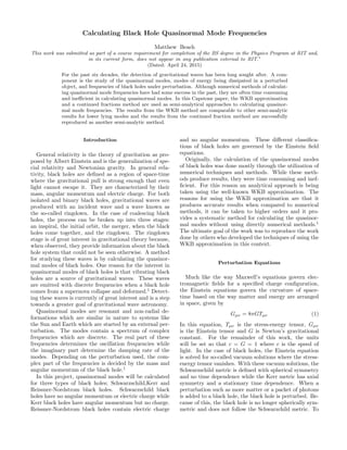
culated values to. Finally, a comparison between orders
is shown in the following plot.In this figure l = 1 and n

5. 5
is varied in order to show how increasing n with a fixed
causes more error in the di↵erent orders of approxima-
tion.
0.1 0.2 0.3 0.4 0.5 0.6 0.7 0.8
0
0.1
0.2
0.3
0.4
0.5
0.6
0.7
0.8
0.9
1
Re(σ)
Im(σ)
Comparing Orders to Semi−Analytic Results
First Order
Second Order
Third Order
Semi−Analytic
WKB Conclusions
The WKB approximation was utilized for the pur-
pose of calculating quasinormal frequencies of a per-
turbed Schwarzchild metric. Data was calculated from
a first, second and third-order WKB approximation and
compared percentage wise to previously obtained semi-
analytic data by a method of continued fractions.4
For all
orders, a fixed l and increasing n caused more error while
fixed n and increasing l caused less error. Also, increas-
ing order caused less percentage error when compared
to semi-analytic data. To add, even with the approxima-
tion taken out to increasingly higher orders, it eventually
breaks down as quasinormal frequencies are taken out to
higher values of n. At the same time, the frequency val-
ues gain accuracy with increasing l. As a result, the
WKB approximation provides a consistently more reli-
able method for calculating quasinormal frequencies as
the method is taken out to higher orders. In Capstone
II, quasinormal frequencies will be calculated using a con-
tinued fraction method and then compared to the results
of the WKB approximation method and previously calcu-
lated semi-analytic results.4
In the following sections, this
semi-analytical method involving continued fractions will
be utilized to calculate quasinormal mode frequencies to
reproduce the results of Leaver4
and the resultant values
will be compared to the results of the WKB method.
Continued Fractions
A second method that can be used to calculate quasi-
normal mode frequencies is by solving Eq. (5) but with a
direct analytical method. In the case of a non-rotating,
non-charged black hole, Schwarzschild coordinates are
chosen along with the function (t, r, ✓, ) denoting the
perturbation to a spin s field4
. The function can be
Fourier analyzed and expanded in spherical harmonics
as:
(t, r, ✓, ) =
1
2⇡
Z 1
1
e i!t
X
l
1
r
(r, !)Ylm(✓, )d!
(13)
The ordinary di↵erential equation that is satisfied by
can be written in a modified form of Eq. (5):
r(r 1)
d2
dr2
+
d
dr
+ (
!2
r3
r 1
l(l + 1) +
✏
r
) = 0 (14)
Where ! is the complex frequency oscillation, l is the
angular harmonic index and ✏ is one minus the square of
the field’s spin weight and has values of 1, 0, 3 if is a
component of a scalar, electromagnetic or gravitational
field respectively4
. This ✏ is the same as from the WKB
method but with a sign di↵erence. In this context, the
spin weight field is denoted by s and is 0, 1 or 2 if cor-
responds to a scalar, electromagnetic or gravitations field
respectively. Eq. (14) is an ordinary di↵erential equation
of second order with two regular singular points and one
irregular singular point4
. A regular singular point corre-
sponds to a point where a coe cient in the di↵erential
equation diverges at the limit of that point but remains
finite if the coe cient is multiplied by a monomial with
a root at the singular point. For Eq. (14), the regular
singular points are at r = 0 and r = 1. An irregular
singular point also has diverging coe cients but diverge
more rapidly then one over the coordinate minus the sin-
gular point. For Eq. (14), the irregular singular point is
at r = 1. A di↵erential equation of this form is a mem-
ber of a group of di↵erential equations called generalized
spheroidal wave equations4
. The general form of these
wave equations take a general form of:
x(x x0)d2
y
dx2 + (B1 + B2x)dy
dx
+( 2
x(x x0) 2µ (x x0) + B3)y = 0 (15)
where B1, B2, B3, , µ and x0 are constants. In the con-
text of this project, Eq. (14) can be put into the form of a
generalized spheroidal wave equation by the substitution
of:
= r1+s
(r 1) i!
y (16)
Once this substitution is made, a di↵erential equation
for y can be made in the form of a generalized spheroidal
wave equation. After the substitution is made, the coef-
ficients outside of the the derivatives of the new function
y are arranged so that the new di↵erential equation is
a generalized spheroidal wave equation with two regular
singular points and one irregular singular point. After
this substitution, Eq. (16) takes the form:

6. 6
r(r 1)d2
y
dr2 + [2(s + 1 i!)r (2s + 1)]dy
dr
+[!2
r(r 1) + 2!2
(r 1) + 2!2
l(l + 1) + s(s + 1) (2s + 1)i!]y = 0 (17)
Using this di↵erential equation of y, it can be reasoned
that the use of a power series expansion for a di↵erential
equation about a regular singular point usually has a
radius of convergence equivalent to the distance from the
nearest singular point to the point of expansion. Also, the
singular point at r = 0 interferes with the convergence of
a power series from 1 to infinity. To avoid this problem,
the singular points must be moved so that the singular
point at 1 is moved to 0 and the point at infinity is moved
to 1. This can be done with a change of variable where
u = (r 1)/r and by rewriting y as:
y = ei!r
r 1/2B2 i
f(u) (18)
Once again, this new form of y that is related to the
function f is directly substituted into Eq. (18) and the
coe cients outside the derivatives of f are arranged with
new polynomials in terms of terms from Eq. (17) and
the new variable u. With this change of variable and
equation substitution, Eq. (17) can be re-expressed in
the form:
u(1 u)2 d2
f
du2
+(c1+c2u+c3u2
)
df
du
+(c4+c5u)f = 0 (19)
In this di↵erential equation, the new terms multiplied by
the derivatives of f are:
c1 = B2 + B1,
c2 = 2(c1 + 1 + i(µ )),
c3 = c1 + 2(1 + iµ),
c5 = (1
2 B2 + iµ)(1
2 B2 + iµ + 1 + B1),
c4 = c5
1
2 B2(1
2 B2 1) + µ(i µ) + i c1 + B3(20)
The function f is then expanded into a power series of u
of the form:
f(u) =
NX
n=0
anun
(21)
When this power series is put into Eq. (19), the an co-
e cients can be arranged into a three term recurrence
relation of the form:
↵0a1 + 0a0 = 0
↵nan+1 + nan + nan 1 = 0, n = 1, 2, ... (22)
In this three term recurrence relation, the ↵, , and
are represented by the index n and terms from the gen-
eralized spheroidal wave equation. The terms from the
generalized spheroidal wave equation come from the var-
ious c terms from Eq. (19) and re-writing them in terms
of the wave equation coe cients as in Eq. (20). After
this arrangement is made, ↵, , and take the form:
↵n = (n + 1)(n + B2 + B1),
n = 2n2
2(B2 + i(µ ) + B1)n
(1
2 B2 + iµ)(B2 + B1) + i (B1 + B2) + B3,
n = (n 1 + 1
2 B2 + iµ)(n + 1
2 B2 + iµ + B1) (23)
In the context of the di↵erential equation, Eq. (17), the
terms in the three term recurrence coe cients which
came from the generalized spheroidal wave equation can
be expressed in terms of variables from Eq. (17). When
these terms are related, the generalized spheroidal wave
equation terms are written as:
µ = !,
= !,
B1 = ( 2s 1),
B2 = (2s 2i! + 2),
B3 = (2!2
l(l + 1) + s(s + 1) 2is! i!) (24)
Substituting these values into the coe cients of the three
term recurrence relation, the coe cients simplify to func-
tions of n, l, ✏ and ! and take the form:
↵n = n2
+ ( 2i! + 2)n 2i! + 1,
n = (2n2
+ ( 8i! + 2)n 8!2
4i! + l(l + 1) ✏),
n = n2
4i!n 4!2
✏ 1 (25)
In Eq. (14), a boundary condition is invoked such that
as approaches spatial infinity, goes as ri!
ei!r5
. This
boundary condition is satisfied when ! = !n which corre-
sponds to the quasinormal mode frequencies. This is only
true when the power series coe cients in Eq. (21) are ab-
solutely convergent which is true when the sum over all
an exists and is finite. By the theory of three term re-
currences, conditions can be set for which the sum of the
power series coe cients converges absolutely. For large
values of n, the power series coe cients take the limit:
an+1
an
! 1 ±
2i!1/2
n1/2
+
2i! 3/4
n
+ ... (26)
In order for the sum of power series coe cients to con-
verge absolutely, the minus sign must be used in Eq. (26)
which will only occur for values of ! that correspond to
quasinormal mode frequencies6
. The power series coe -
cients must then form a solution to the three term recur-
rence relation which is minimal as n goes to infinity6
. If
the power series coe cients do not form a minimal solu-
tion sequence, the resultant ratio of coe cients will not

7. 7
have a zero radius of convergence and therefore diverge.
From these conditions, taking a ratio of successive power
series coe cients produces an infinite continued fraction
of the form in Eq. (27) that is convergent as n goes to
infinity4
. To get this continued fraction, a ratio of power
series coe cients is defined as:
rn =
an+1
an
(27)
Then, dividing Eq. (22) by an yields:
↵nrn + n +
n
rn 1
= 0 (28)
Rearranging this equation gives the following recur-
rence relation:
rn 1 =
n
n + ↵nrn
(29)
When this recurrence is repeated, an infinite continued
fraction is made of the form:
an+1
an
=
n+1
n+1
↵n+1 n+2
n+2
↵n+2 n+3
n+3 ...
(30)
It is convenient to use the notation:
an+1
an
=
n+1
n+1
↵n+1 n+2
n+2
↵n+2 n+3
n+3
... (31)
Eq. (31) can be considered a boundary condition on n
as it approaches infinity for the sum of the power se-
ries coe cients. This is a result of the large n limit
in Eq. (26) where the ratio of power series coe cients
converges. A characteristic equation for the quasinor-
mal mode frequencies can be found by setting n = 0 in
Eq. (31) and setting it equal to the initial condition for
the three term recurrence relation in Eq. (22) for the ratio
of a1/a0. Therefore the following equations must hold:
a1
a0
=
0
↵0
(32)
With this condition, the continued fraction in Eq. (31)
evaluated at n = 0 can be written the form:
a1
a0
=
1
1
↵1 2
2
↵2 3
3
... (33)
By equating the right hand sides of Eq. (32) and Eq. (33)
an implicit characteristic equation of the quasinormal
mode frequencies can be expressed as:
0 = 0
↵0 1
1
↵1 2
2
↵2 3
3
... (34)
Eq. (34) can be inverted any number of times to pro-
duce an equation relating a finite continued fraction to
an infinite continued fraction which is written as:
n
↵n 1 n
n 1
↵n 2 n 1
n 2
... ↵0 1
0
= ↵n n+1
n+1
↵n+1 n+2
n+2
↵n+2 n+3
n+3
... (35)
For all positive n, Eq. (34) and Eq. (35) are entirely
equivalent in the sense that all roots of Eq. (34) are also
roots of Eq. (35) and all roots of Eq. (35) are roots of
Eq. (34)4
. Both equations can be used as a defining
equation for quasinormal mode frequencies, !n, for the
Schwarzchild metric. Calculating the quasinormal mode
frequencies can now be accomplished by numerically find-
ing the roots of either Eq. (34) or Eq. (35). Once a value
is picked for the parameters n, l and ✏, the ↵, and
in the continued fractions become polynomials of only !.
The continued fractions can then be expressed as polyno-
mials of ! where the roots can be calculated numerically.
Due to the fact that Eq. (34) is an infinite continued
fraction where each continuant is a function of the quasi-
normal frequencies, it can be reasoned that there exists
an infinite number of frequencies, though no formal proof
of this has been presented.
Continued Fractions Results
After using semi-analytical methods to solve Eq. (14),
the calculation of Schwarzchild quasinormal mode fre-
quencies was reduced to finding the roots of either
Eq. (34) or Eq. (35) which was accomplished numerically
through the use of Mathematica. Through these numer-
ical calculations, it can be confirmed that the roots of
Eq. (34) are indeed equivalent to the roots of Eq. (35).
Also, due to the fact that both characteristic equations
involve the use of infinite continued fractions, finding the
roots of either equation must be done by truncating the
infinite continued fraction at a particular continuant and
calculating the root of the resulting finite continued frac-
tions. In the following figures, frequencies were calcu-
lated using either characteristic equation at higher and
higher continuant truncations.
This data shows that as roots are calculated for ei-
ther characteristic equation, the accuracy of the calcu-
lated quasinormal mode frequencies become increasingly
higher when compared to the values calculated by Leaver
as the continued fractions are taken to higher trunca-
tions. However, when quasinormal mode frequencies are
calculated using Eq. (35), calculating higher mode quasi-
normal frequencies must be done by going out to higher
and higher truncations of the continuant of the infinite
continued fraction part of the equation to become accu-
rate compared to the results of Leaver. A result of this
need for higher truncations is that the code created to
calculate quasinormal mode frequencies takes longer to

8. 8
1 2 3 4 5 6 7 8 9 10
0.68
0.69
0.7
0.71
0.72
0.73
0.74
0.75
Number of Continuants
Re(ω)
Comparing Truncated Values ofω to Expected Value
Calculated Values
Expected Value
compute values as the root is found at higher continu-
ants. An example of this result is shown in the following
figure for the calculation of a higher mode frequency.
Compared to the calculation of higher mode quasi-
normal mode frequencies using Eq. (35), calculations of
higher mode frequencies using Eq. (34) do not need to
be taken out to higher numbers of continuants for the
same accuracy obtained for the lower lying quasinormal
frequencies. This result is shown in the following fig-
ure of the calculation of a higher mode frequency using
Eq. (34).
10 15 20 25 30 35 40 45 50
0.1265
0.127
0.1275
0.128
0.1285
0.129
0.1295
0.13
Number of Continuants
Re(ω)
Truncated Values at n = 10 of Eq. 34 Compared to Expected Value
Calculated Values
Expected Value
Even though calculating higher mode quasinormal fre-
quencies using Eq. (35) requires higher truncations for
increased accuracy, both characteristic equations can be
used to calculate frequencies for any value of n, l or ✏.
This is the same as the results of the WKB method with
the di↵erence that what was called in the WKB method
is now called ✏ in the continued fraction method. The val-
ues for the respective field being used for in the WKB
method and the values for the respective field used for ✏ in
the continued fraction method do di↵er by a negative sign
for scalar, electromagnetic and gravitational fields. From
the calculation of various quasinormal mode frequencies,
a few trends emerged depending on the variation of the
input parameters. For instance, for a fixed value of l and
increasing value of n, the real part of the calculated fre-
quency varies only slightly while the imaginary part of
the frequencies increases directly with increasing values
of n. Conversely, when n is fixed and l is increasing, the
real part of the quasinormal mode frequencies increases
while the imaginary part varies only slightly in compari-
son. These results are illustrated in the following figures.
Continued Fractions Conclusions
After solving Eq. (14) analytically with a continued
fraction method and using numerical techniques to cal-
culate the quasinormal mode frequencies of the resulting
continued fractions, some conclusions can be drawn from
this method. First, two equations, Eq. (34) and Eq. (35)
can be used to calculate the quasinormal mode frequen-
cies for the Schwarzchild metric. Both equations can be
used to converge in accuracy to the resultant quasinormal
mode frequencies calculated by Leaver. However, cal-
culating quasinormal frequencies at higher modes with

9. 9
0 0.1 0.2 0.3 0.4 0.5 0.6 0.7 0.8
0
0.5
1
1.5
2
2.5
3
3.5
4
4.5
5
Re(ω)
Im(ω)
l = 2, n from 1 to 10 Quasinormal Mode Frequencies
0.5 1 1.5 2 2.5 3 3.5 4 4.5 5
0.176
0.178
0.18
0.182
0.184
0.186
0.188
0.19
Re(ω)
Im(ω)
n = 1, l from 2 to 12 Quasinormal Mode Frequencies
Eq. (35) requires taking the infinite continued fraction
part of the equation out to higher truncations which dras-
tically increases computational time when compared to
calculated higher mode frequencies with Eq. (34). Also,
regardless of whether Eq. (34) or Eq. (35) is used to calcu-
lated quasinormal mode frequencies, trends emerge with
varying values of n and l. With fixed l and increasing
n, the imaginary part of the quasinormal frequency in-
creases with n while the real part of the frequency only
varies slightly in comparison. On the other hand, with
fixed n and increasing l, the real part of the frequency
increases with l while the imaginary part varies only
slightly in comparison.
Conclusions
In conclusion, detecting gravitational waves has been
of great interest in the study of gravitation. In the case of
either isolated or binary black holes, gravitational waves
are created with an incident wave and an outgoing wave
known as the ringdown. Calculating quasinormal mode
frequencies is of importance in the field of general rela-
tivity as a method of studying the ringdown portion of
gravitational waves since they provide information about
the ringdown phase of gravitational waves. This can pro-
vide insight about the black hole system that is being ob-
served experimentally. In the scope of this project, two
methods were employed to calculate quasinormal mode
frequencies of Schwarzschild black holes; one involving
the use of the WKB approximation and the other involv-
ing the use of continued fractions. Both methods have
positive and negative aspects associated with them. In
the case of the WKB approximation method, positive
aspects are as follows. The analytical aspect of solving
the di↵erential equation with the WKB approximation is
straight forward and less involved than that of the con-
tinued fraction method. Also, when the analytical por-
tion of the WKB method is complete, the computational
aspect of calculating the values involves very little com-
putational time with calculating quasinormal mode fre-
quencies. To add, there are also negative results of using
the WKB method. While solving the di↵erential equa-
tion is more straight forward with the WKB method, in
order to get increasingly accurate calculations, the WKB
approximation needs to be taken out to higher orders
which becomes increasingly more time consuming. And
even with the approximation taken out to higher orders,
the calculated quasinormal mode frequencies still lose ac-
curacy at higher mode numbers when compared to other
semi-analytical results since the potential in Eq. (5) is
approximated by a Taylor series instead of solving the
di↵erential equation more directly. This also causes the
calculation of higher mode frequencies with the WKB
method to be taken out to higher orders which still lose
accuracy when taken to infinitely higher modes. Like the
WKB method, the continued fraction approach to calcu-
lating quasinormal frequencies has positive and negative
results. While the continued fraction method does use
an approximation when solving the di↵erential equation
with a power series method in order to calculate quasinor-
mal mode frequencies, infinitely higher mode frequencies
can be calculated by simply going to higher truncations
of the continued fractions instead of going to higher and
higher orders. While this is an advantage compared to
the WKB method, the process of solving the di↵eren-
tial equation with the continued fraction method is more
detailed and di cult to accomplish. But because the
di↵erential equation is solved more directly, there is no
restriction on going to out to higher mode calculations of
quasinormal frequencies unlike with the WKB method.
To add, the computational time needed with the contin-
ued fraction method can be much longer than that of the
WKB method; especially when higher mode quasinormal
frequencies are being calculated. In the end, calculating
higher mode frequencies takes more time to complete for
both methods. For the calculation of lower mode fre-
quencies, the WKB method should be employed and can
be used to give estimates for the roots of the equations
used in the continued fraction method. For the calcula-
tion of higher mode frequencies, the continued fraction

10. 10
method should be used in order to gain more accuracy
when compared to the purely numerically obtained quasi-
normal mode frequencies. In addition to each method
providing positive and negative results when calculating
quasinormal mode frequencies, they each also give rise to
trends in the calculation of said frequencies. Both meth-
ods can be used to calculate frequencies given a specific
set of parameters for mode number, angular harmonic
index and spin weight field number. Also, both methods
can be used to study trends in the calculation of quasi-
normal mode frequencies when these parameters are var-
ied. To end, the use of either method provides insight
about the e↵ectiveness of each method in terms of the
analytic and numerical aspects of each as well as trends
that occur between the various calculated quasinormal
mode frequencies.
Acknowledgments
I’d like to thank Dr. Linda Barton for heading the Cap-
stone Committee, all members of the Capstone Commit-
tee, Dr. Eric West for being my primary advisor and Dr.
Edwin Hach for being my secondary advisor.
⇤
Rochester Institute of Technology, School of Physics and
Astronomy, Faculty Advisor: Dr. Eric West
1
B. F. Schutz and C. M. Will, Astrophys.J. 291, L33 (1985).
2
T. Regge and J. A. Wheeler, Phys.Rev. 108, 1063 (1957).
3
S. Iyer and C. M. Will, (1986).
4
E. Leaver, Proc.Roy.Soc.Lond. A402, 285 (1985).
5
W. G. Baber and H. R. Hass, Mathematical Proceedings of
the Cambridge Philosophical Society 31, 564 (1935).
6
W. Gautschi, SIAM Review 9, 24 (1967).