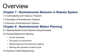
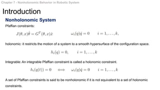
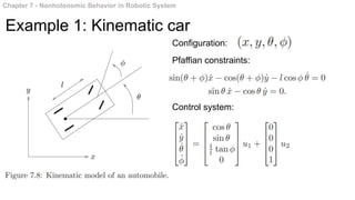
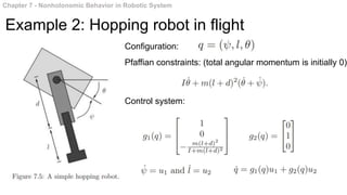
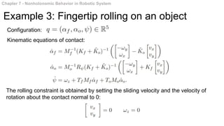
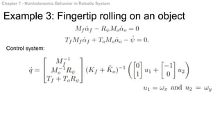
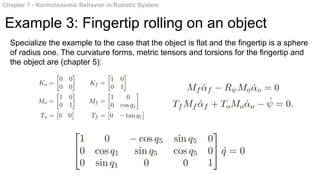
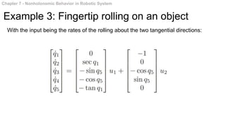
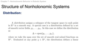
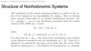
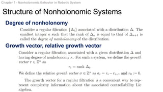
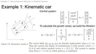
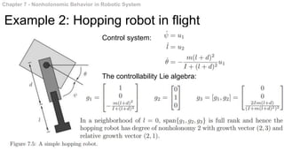
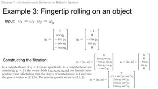
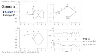
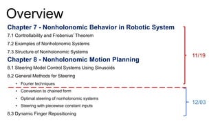
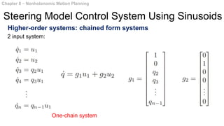
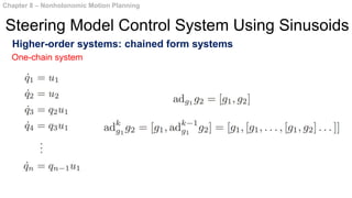
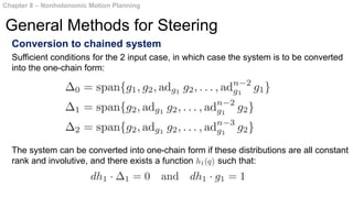
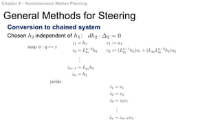
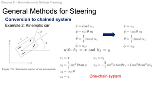
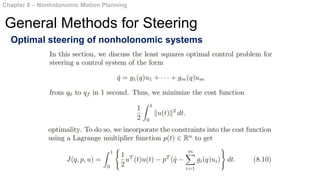
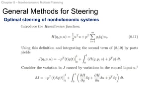
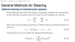
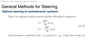
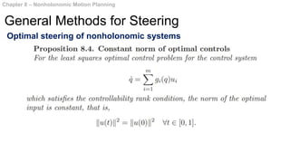
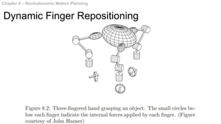
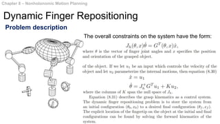
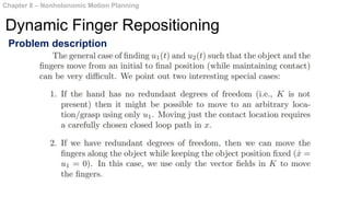
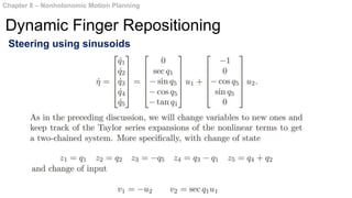
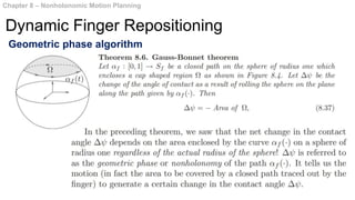
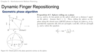
A Mathematical Introduction to Robotic Manipulation 第7&8章

A mathematical introduction
to robotic manipulation
Chapter 7&8
Harada Lab, Osaka university
D2 Zhenting Wang
2021.11.19

Overview
Chapter 7 - Nonholonomic Behavior in Robotic System
7.1 Controllability and Frobenius’ Theorem
7.2 Examples of Nonholonomic Systems
7.3 Structure of Nonholonomic Systems
Chapter 8 - Nonholonomic Motion Planning
8.1 Steering Model Control Systems Using Sinusoids
8.2 General Methods for Steering
• Fourier techniques
• Conversion to chained form
• Optimal steering of nonholonomic systems
• Steering with piecewise constant inputs
8.3 Dynamic Finger Repositioning

Overview
7.1 Controllability and Frobenius’ Theorem
7.2 Examples of Nonholonomic Systems
7.3 Structure of Nonholonomic Systems
Chapter 8 - Nonholonomic Motion Planning
8.1 Steering Model Control Systems Using Sinusoids
8.2 General Methods for Steering
• Fourier techniques
• Conversion to chained form
• Optimal steering of nonholonomic systems
• Steering with piecewise constant inputs
8.3 Dynamic Finger Repositioning
11/19
12/03

Nonholonomic System
Pfaffian constraints:
holonomic: it restricts the motion of a system to a smooth hypersurface of the configuration space.
Integrable: An integrable Pfaffian constraint is called a holonomic constraint.
A set of Pfaffian constraints is said to be nonholonomic if it is not equivalent to a set of holonomic
constraints.
Introduction

Nonholonomic System
In this chapter:
Understand when we can exploit the nonholonomy of the constraints to achieve motion between
configurations.
Examples:
Introduction

Lie derivative and Lie bracket

Two kinds of situations:
1. Bodies in contact with each other which roll without slipping
• Dextrous manipulation with a multi-fingered robot hand
• Path planning for mobile robots or automobiles
2. Conservation of angular momentum in a multibody system
• Motion of a satellite with robotic appendages moving in space
Examples of Nonholonomic Systems

Example 1: Kinematic car
Configuration:
Pfaffian constraints:
Control system:

Example 2: Hopping robot in flight
Configuration:
Pfaffian constraints: (total angular momentum is initially 0)
Control system:

Example 3: Fingertip rolling on an object
Configuration:
Kinematic equations of contact:
The rolling constraint is obtained by setting the sliding velocity and the velocity of
rotation about the contact normal to 0:

Control system:

Specialize the example to the case that the object is flat and the fingertip is a sphere
of radius one. The curvature forms, metric tensors and torsions for the fingertip and
the object are (chapter 5):

With the input being the rates of the rolling about the two tangential directions:

Distribution:
Structure of Nonholonomic Systems

Degree of nonholonomy
Growth vector, relative growth vector

Control system:
To calculate the growth vector, we build the filtration:

Control system:
The controllability Lie algebra:

Input:
Constructing the filtration:

Optimal control
By attaching a cost functional to each trajectory, we can limit our search of trajectories
which minimize a cost function.
Typical cost functions might be the length of the path, the control cost, or the time
required to execute the trajectory.
Piecewise constant inputs
The most naive way of using constant inputs is to pick a time interval and generate a
graph by applying all possible sequences of input. Each node on the graph
corresponds to a configuration, and branches indicate the choice of a fixed control
over the time interval.
Chapter 8 – Nonholonomic Motion Planning
Introduction

Canonical paths
This approach solves the nonholonomic path planning problem by choosing a family
of paths which can be used to produce desired motions.
The set of canonical paths used for a given problem is usually specific to that problem.
In some cases the paths may derived from some unifying principle.
Introduction

First-order controllable systems: Brockett’s system
Steering Model Control System Using Sinusoids

Case:

Case:
Total cost:

Case: input m

Control Algorithm:

Second-order controllable systems
By computation:
The maximum number of controllable is :

Control Algorithm:

Control Algorithm:
m=2

Higher-order systems: chained form systems (12/03)
Generalization: conversion to chained form

Fourier techniques
General Methods for Steering
Control equations:

Fourier techniques

Fourier techniques
Step C:

Higher-order systems: chained form systems
2 input system:
One-chain system

Higher-order systems: chained form systems
One-chain system

Conversion to chained system
Control system:
The system is in chained form in the z
coordinates with input v.

The system can be converted into one-chain form if these distributions are all constant
rank and involutive, and there exists a function such that:
Sufficient conditions for the 2 input case, in which case the system is to be converted
into the one-chain form:

Chosen independent of :

One-chain system

Optimal steering of nonholonomic systems

The solution of this equation is of the form:
Example: Optimal inputs of Engel’s system

The optimal inputs for the Engel’s system come from elliptic function.
Example: Optimal inputs of Engel’s system
Elliptic integral

Steering with piecewise constant inputs
We consider a nilpotent Lie algebra of order k generated by the vector fields
The Philip Hall basis of the controllability Lie algebra generated by are
defined as

All flows of the nonlinear control system:
are of the form
for some suitably chosen functions known as the Philip Hall coordinates.
The mean of (8.22) is:
All flows that could possibly be generated by the control system may be obtained by
composing flows along the Philip Hall basis elements

satisfies a differential equation involving the basis elements:

Differentiating equation:
We introduced the notation:

Example: Nilpotent system of degree three with two inputs

Dynamic Finger Repositioning

Problem description
The overall constraints on the system have the form:

Problem description

Steering using sinusoids

Steering using sinusoids
The location of the contact on
the finger is unchanged
The location of the contact on
the face of the object

Geometric phase algorithm

A Mathematical Introduction to Robotic Manipulation 第7&8章

More Related Content

What's hot

Similar to A Mathematical Introduction to Robotic Manipulation 第7&8章

Recently uploaded

A Mathematical Introduction to Robotic Manipulation 第7&8章

Editor's Notes