power point of robotics Robotics is the interdisciplinary study and practice of the design, construction, operation, and use of robots. Within mechanical engineering, robotics is the design and construction of the physical structures of robots, while in computer science, robotics focuses on robotic automation algorithms.

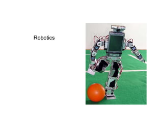
1. Robotics

2. “A robot is a reprogrammable, multifunctional manipulator
designed to move material, parts, tools, or specialized devices
through variable programmed motions for the performance of
a variety of tasks.” (Robot Institute of America)
Definition:
Alternate definition:
“A robot is a one-armed, blind idiot with limited memory
and which cannot speak, see, or hear.”

3. Ideal Tasks
Tasks which are:
– Dangerous
• Space exploration
• chemical spill cleanup
• disarming bombs
• disaster cleanup
– Boring and/or repetitive
• Welding car frames
• part pick and place
• manufacturing parts.
– High precision or high speed
• Electronics testing
• Surgery
• precision machining.

4. Automation vs. robots
• Automation –Machinery designed to carry out a specific task
– Bottling machine
– Dishwasher
– Paint sprayer
• Robots – machinery designed
to carry out a variety of tasks
– Pick and place arms
– Mobile robots
– Computer Numerical Control
machines

5. Types of robots
• Pick and place
– Moves items between points
• Continuous path control
– Moves along a programmable path
• Sensory
– Employs sensors for feedback

6. Pick and Place
• Moves items from one point to
another
• Does not need to follow a specific
path between points
• Uses include loading and
unloading machines, placing
components on circuit boards, and
moving parts off conveyor belts.

7. Continuous path control
• Moves along a specific path
• Uses include welding, cutting,
machining parts.

8. Sensory
• Uses sensors for feedback.
• Closed-loop robots use sensors in
conjunction with actuators to gain
higher accuracy – servo motors.
• Uses include mobile robotics,
telepresence, search and rescue, pick
and place with machine vision.

9. Measures of performance
• Working volume
– The space within which the robot operates.
– Larger volume costs more but can increase the capabilities of a
robot
• Speed and acceleration
– Faster speed often reduces resolution or increases cost
– Varies depending on position, load.
– Speed can be limited by the task the robot performs (welding,
cutting)
• Resolution
– Often a speed tradeoff
– The smallest step the robot can take

10. • Accuracy
–The difference between the
actual position of the robot and
the programmed position
• Repeatability
Will the robot always return to the
same point under the same
control conditions?
Increased cost
Varies depending on position,
load
Performance (cont.)

11. Control
•Open loop, i.e., no feedback, deterministic
•Closed loop, i.e., feedback, maybe a sense of
touch and/or vision

12. • Degrees of freedom—number of independent motions
– Translation--3 independent directions
– Rotation-- 3 independent axes
– 2D motion = 3 degrees of freedom: 2 translation, 1 rotation
– 3D motion = 6 degrees of freedom: 3 translation, 3 rotation
Kinematics and dynamics

13. • Actions
– Simple joints
• prismatic—sliding joint, e.g., square cylinder in square tube
• revolute—hinge joint
– Compound joints
• ball and socket = 3 revolute joints
• round cylinder in tube = 1 prismatic, 1 revolute
• Mobility
– Wheels
– multipedal (multi-legged with a sequence of actions)
Kinematics and dynamics (cont.)

14. Kinematics and dynamics (cont.)
• Work areas
– rectangular (x,y,z)
– cylindrical (r,,z)
– spherical (r,,)
• Coordinates
– World coordinate frame
– End effector frame
– How to get from coordinate system x” to x’ to x
x
x''
x'

15. Transformations
• General coordinate transformation from x’ to x is x = Bx’ + p ,
where B is a rotation matrix and p is a translation vector
• More conveniently, one can create an augmented matrix
which allows the above equation to be expressed as x = A x’.
• Coordinate transformations of multilink systems are represented as
x0 = A01 A12A23. . .A(n-1)(n)xn

16. Dynamics
• Velocity, acceleration of end actuator
– power transmission
– actuator
• solenoid –two positions , e.g., in, out
• motor+gears, belts, screws, levers—continuum of positions
• stepper motor—range of positions in discrete increments

17. A 2-D “binary” robot segment
• Example of a 2D robotic link having three solenoids to
determine geometry. All members are linked by pin joints; members
A,B,C have two states—in, out—controlled by in-line solenoids.
Note that the geometry of such a link can be represented in terms of
three binary digits corresponding to the states of A,B,C, e.g., 010
represents A,C in, B out. Links can be chained together and
controlled by sets of three bit codes.
A C
B A C
B A C
B A C
B
A C
B A C
B
A C
B A C
B

18. Problems
• Joint play, compounded through N joints
• Accelerating masses produce vibration, elastic deformations in links
• Torques, stresses transmitted depending on end actuator loads

19. Control and programming
• Position of end actuator
– multiple solutions
• Trajectory of end actuator: how to get from point A to B
– programming for coordinated motion of each link
– problem—sometimes no closed-form solution

20. Control and programming (cont.)
• Example: end actuator (tip) problem with no closed solution.
Two-segment arm with arm lengths L1 = L2, and stepper -motor
control of angles 1 and 2.
Problem: control 1 and 2 such that arm tip traverses its range at
constant height y, or with no more variation than y.
Geometry is easy: position of arm tip
x = L1 (cos 1 + cos 2)
y = L1 (sin 1 + sin 2)
1
2
L1
L2
y

21. Control and programming (cont.)
• Arm tip moves by changing 1 and 2 as a function of time.
Therefore
So, as 1 and 2 are changed, x and y are affected.
To satisfy y = constant, we must have
. So the rates at which 1 and 2 are changed depend on the values of
1 and 2.
)
sin
(sin 2
2
1
1
1 


 

 

 L
x
0
)
cos
(cos 2
2
1
1
1 

 


 

 L
y
2
1
1
2
cos
cos



 
 


22. Control and programming (cont.)
There is no closed-form solution to this problem. One must use
approximations, and accept some minor variations in y. Moving the
arm tip through its maximum range of x might have to be
accomplished through a sequence of program steps that define
different rates of changing 1 and 2.
• Possible approaches:
– Program the rates of change of 1 and 2 for y = const. for initial
values of 1 and 2 . When arm tip exceeds y, reprogram for
new values of 1 and 2.
– Program the rates of change of 1 and 2 at the initial point and
at some other point for y = const. Take the average of these two
rates, and hope that y is not exceeded. If it is exceeded,
reprogram for a shorter distance. Continue program segments
until the arm tip has traversed its range.
•

23. Control and programming (cont.)
– Program the rates of change of 1 and 2 at the initial point and
at some other point for y = const. Take the average of these two
rates, and hope that y is not exceeded. If it is exceeded,
reprogram for a shorter distance. Continue program segments
until the arm tip has traversed its range.
– The rate of change of 1 and 2 can be changed in a
programming segment, i.e., the rates of change need not be
uniform over time. This programming strategy incorporates
approaches 1) and 2). Start with rates of change for the initial
values of 1 and 2 , then add an acceleration component so that
y = const. will also be satisfied at a distant position.

24. Feedback control
• Rotation encoders
• Cameras
• Pressure sensors
• Temperature sensors
• Limit switches
• Optical sensors
• Sonar

25. New directions
• Haptics--tactile sensing
• Other kinematic mechanisms,
e.g. snake motion
• Robots that can learn