This document presents a model of the job search process based on two character measures - attractiveness and character. Attractiveness is easily observable but character requires an interview. The model considers job seekers deciding whether to apply for jobs and employers deciding whether to invite applicants for interviews. If invited, both parties observe each other's character and decide whether to make an offer/accept. The goal is to find a Nash equilibrium strategy profile satisfying certain criteria like mutual acceptance being required and decisions maximizing expected rewards from search. Multiple equilibria may exist.

1. A LABOUR MARKET MODEL WITH MULTIPLE CRITERIA
DAVID M. RAMSEY AND STEPHEN KINSELLA
Abstract. We develop a job search model based on two character measures. One
measure describes the ‘attractiveness’ of an individual or position. It is assumed that
preferences are common according to this measure: i.e. each employer prefers highly
attractive job seekers and all employers agree as to which job seekers are attractive.
Preferences are homotypic with respect to the second measure, referred to as ‘character’
i.e. all job seekers prefer jobs of a similar character. It is assumed that attractiveness is
easy to measure and observable with certainty, but in order to observe the character of
a prospective employee or position, it is necessary to interview. Hence, on receiving an
application from a prospective employee, an individual employer must decide whether
to interview them to gauge their suitability for the position. Job matching only occurs
after an interview. During the interview phase of the process, the employer and job
searcher observe each other’s character, and then decide whether to make a job offer
or accept a job offer, respectively. It is assumed that mutual acceptance is required
for employment to occur. This paper presents a model of the job search process, and
gives a procedure for finding a Nash equilibrium which satisfies a set of criteria based on
the concept of subgame perfection. Two examples are presented, and it is shown that
multiple equilibria may exist. Further work will concentrate on simulating this process
for realistic parameters.
Date: February 19, 2009.
Key words and phrases. Evolutionary game theory, Job Search, Common preferences, Homotypic
preferences, Subgame perfection. JEL Codes: D83, J00, J20, J41, J62.
1

2. 2
A Labour Market Model with Multiple Criteria
Abstract. We develop a job search model based on two character measures. One
measure describes the ‘attractiveness’ of an individual or position. It is assumed that
preferences are common according to this measure: i.e. each employer prefers highly
attractive job seekers and all employers agree as to which job seekers are attractive.
Preferences are homotypic with respect to the second measure, referred to as ‘character’
i.e. all job seekers prefer jobs of a similar character. It is assumed that attractiveness is
easy to measure and observable with certainty, but in order to observe the character of
a prospective employee or position, it is necessary to interview. Hence, on receiving an
application from a prospective employee, an individual employer must decide whether
to interview them to gauge their suitability for the position. Job matching only occurs
after an interview. During the interview phase of the process, the employer and job
searcher observe each other’s character, and then decide whether to make a job offer
or accept a job offer, respectively. It is assumed that mutual acceptance is required
for employment to occur. This paper presents a model of the job search process, and
gives a procedure for finding a Nash equilibrium which satisfies a set of criteria based on
the concept of subgame perfection. Two examples are presented, and it is shown that
multiple equilibria may exist. Further work will concentrate on simulating this process
for realistic parameters.
1. Introduction
This paper presents a model of job search involving both common and homotypic
preferences. All employers prefer job seekers with high qualifications who have a similar
character to themselves. Similarly, all employees prefer attractive positions which have a
similar character to themselves.
For convenience, it is assumed that job searchers and employers know their own qual-
ifications and character with certainty. The distribution of character and qualifications
are assumed to be discrete, and constant over time. Analogous assumptions are made
regarding the distribution of the attractiveness and character of positions. When consid-
ering both job seekers and positions together, the qualifications of a job seeker will be
also referred to as his attractiveness.
Together, the attractiveness, character and the role (employee/employer) of an indi-
vidual determines their ‘type’. Job seekers can observe the attractiveness and character
of prospective jobs perfectly. A job’s attractiveness can be observed very quickly from
an advert. The qualifications of a job seeker are readily seen from his/her application.
However, in order to measure character, an interview is required. It is assumed that each
party incurs costs when they agree on an interview. At each stage of the process, job
searchers and employers incur the costs of not working and not having a position filled,
respectively. The job seeker incurs a cost in applying for a job.
At each stage of the process a job seeker is paired with a position. The job seeker
decides whether to apply for the position on the basis of its attractiveness. The employer
then decides whether to call the applicant to interview on the basis of the application

3. 3
(his attractiveness). A job matching occurs after the interview only by mutual consent.
These final decisions are based on both the attractiveness and character of the prospective
partners. At equilibrium each individual uses a strategy appropriate to their type. The
set of strategies corresponding to such an equilibrium is called an equilibrium strategy
profile.
In the literature to date, job search models typically adopt a matching function ap-
proach, where the employer and employee search for the perfect ‘fit’ using a set of costly
criteria. Equilibrium conditions are derived and tested for robustness once the model is
built, and policy recommendations follow (Burdett, 1978; Pissarides, 1994; Drewlanka,
2006; Shimer and Smith, 2000). Jovanovic (1979), Hey (1982), and MacMinn (1980) are
the classic studies. Devine and Piore (1991) and Shimer and Smith (2000) survey the
more recent developments.
A job can be viewed as an ‘experience good’, where the only way to determine the
quality of a particular match is to form the match and experience it. There have also
been experimental studies done on matching models, for example Roth and Sotomayor
(1990) and many of his subsequent papers1
.
Another strand in the literature is the search-theoretic literature developed by McCall
(1970) and extended by Diamond and Maskin (1979) and others, where the job search
problem is conceived of as a dynamic program which has to be solved in finite time, so
labour markets are best described by optimal control problems and solution methods.
The literature here is vast and well studied.
Job search has also been modelled as a mating or network game, with representa-
tive contributions being (Albelda, 1981; Beller, 1982; Peterson et al., 2000; Coles and
Francesconi, 2007; Fisman et al., 2008; Pissarides, 1994). Our paper’s contribution falls
within this class of models.
The model is presented in Section 2, together with a set of criteria that we wish an
equilibrium to satisfy. These conditions are based on the concept of a subgame perfect
equilibrium. Such an equilibrium is a refinement of the concept of Nash equilibrium.
Section 3 describes a general method for calculating the expected rewards of each
individual under a given strategy profile. Section 4 considers the interview subgame
(when individuals decide whether to offer/take a job or not) and the application/invitation
subgame (when job seekers decide whether to apply for a job and employers decide whether
to invite a job seeker for interview).
Section 5 considers an example. An algorithm for deriving an equilibrium of the required
form is presented. This algorithm uses a greedy search procedure to find a candidate for
a Nash equilibrium and this is followed by policy iteration Velupillai (2000). A simple
example is presented.
1
Basic models start like this: derive a utility function for the worker, U, and have them commit a costly
search to the maximisation of U in finite time. The matching function is the mechanism which equates
workers to firms in this process. Asymmetric information, or educational or skill-based heterogeneity is
then introduced to study an aspect of the labour market process.

4. 4
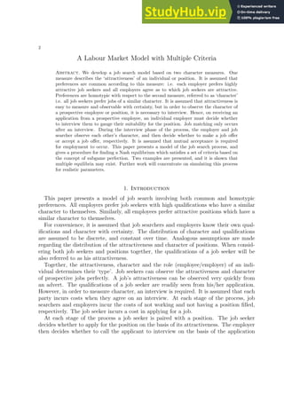
Section 6 presents some results for a larger scale problem, and shows that there may be
multiple equilibria. Section 7 gives a brief conclusion and suggests directions for further
research.
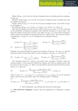
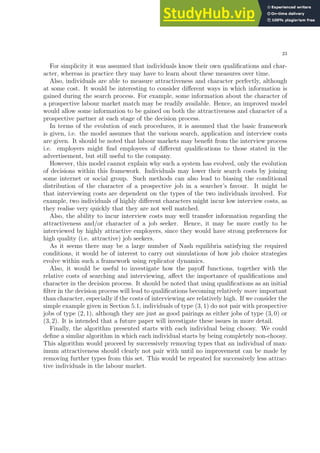
2. The Model
It is assumed that job choice is based on two traits both described by a quantitative
measure. The first will be referred to as ‘attractiveness’ and the second will be referred
to as ‘character’.
We consider a steady state model in which the distributions of the attractiveness (qual-
ifications) and character of a job seeker, as well as of the attractiveness and character
of an employer (denoted X1,js, X2,js, X1,em and X2,em, respectively), do not change over
time.
For convenience, we suppose that X1,es, X1,js, X2,es and X2,js are discrete random
variables which take integer values, and that the attractiveness of a job seeker or employer
is independent of his/her character2
. It will also be assumed that the set of possible
characters of job seekers coincides with the set of possible characters of employers.
The type of an individual can be defined by their attractiveness and character, together
with their role (employer or job seeker). The type of a job seeker will be denoted xjs =
[x1,js, x2,js]. The type of an employer will be denoted xem = [x1,em, x2,em].
Preferences are common with respect to attractiveness, i.e. all job seekers prefer jobs
with a high attractiveness measure3
. Also, preferences are homotypic with respect to
character, i.e., an employer prefers employees with a similar measure of character.
To be more precise, suppose the reward obtained by a type xjs job seeker from taking
a job with a type xem employer is g(x2,js, xem), where g is strictly increasing with respect
to x1,em and strictly decreasing with respect to |x2,js − x2,em|.
Similarly, the reward obtained by a type xem employer from employing a type xjs job
seeker is h(xjs, x2,em), where h is strictly increasing with respect to x1,js, and strictly
decreasing with respect to |x2,js − x2,em|.
The population is assumed to be large.
At each moment n, (n = 1, 2, . . .) each unemployed individual is presented with a
prospective job picked at random. Thus it is implicitly assumed that the operational
ratio of unfilled jobs to job seekers is one, and that individuals can observe as many
prospective jobs as they wish. Suppose the ratio of the number of searching job seekers
to the number of searching employers is r, where r > 1. This situation can be modelled
by assuming that a proportion r−1
r
of employers have attractiveness −∞ (in reality job
seekers paired with such an employer at moment i meet no employer then). An individual
cannot return to a prospective job (or job seeker) found earlier, nor would they want
to, given their preferences and past negative experiences with that prospective employer
(employee).
2In further work we hope to relax this rather restrictive assumption.
3A proxy for which would be the starting wage.

5. 5
Suppose that employees can observe the ‘type’ of a prospective job perfectly. The
attractiveness of an employer can be observed on the basis of an advert, while an interview
is required to observe the character of an employer.
Similarly, an employee’s qualifications can be measured almost instantaneously by em-
ployers on the basis of an application, but in order to observe character an interview is
required.
The (positive) search costs incurred at each stage by a job seeker and by an employer
are c1,js and c1,em, respectively. These reflect the costs of not having a job and not having
a position filled at each stage, respectively. The costs of interviewing are c2,js and c2,em
to job seekers and employers, respectively. The costs of applying for a job are c3,js.
It is assumed that the costs of advertising a vacant position are incorporated into the
costs of not having a position filled. Adverts often give quite explicit information regarding
the qualifications required. It is assumed that this information is implicitly given by the
measure of attractiveness of a job.
Empirical evidence on search costs abounds in the literature, for instance Peterson
et al. (2000) considers job search costs to be the primary cause of ‘sticky’ wages and
low labour market mobility, when contrasting the European and US labour markets.
Devine and Piore (1991) also presents empirical evidence on search costs, and in the
large Lucas/Prescott literature incorporating job search costs into macroeconomic models,
Andolfatto (1996) is representative.
A job seeker first must decide whether to apply for a job or not on the basis of the job
advert (the attractiveness of the job).
If the job seeker applies, the employer must then decide whether to proceed with an
interview or not, based on the qualifications of the job seeker. If either the job searcher
does not apply or the employer does not wish to interview, the two individuals carry
on searching. In some scenarios—for example day by day manual labour—it might pay
individual employers to immediately accept a prospective employee for a job without
interview. However, to keep the strategy space as simple as possible, it is assumed that
individuals must always interview before forming a pair. It should be noted that at
equilibrium a job seeker may implicitly transfer some information about his character by
applying for a job. The importance of this will be considered later in the section on the
application/invitation subgame.
During an interview, an employee observes the character of his prospective employer,
and vice versa. After the interview finishes, both parties must decide whether to accept the
other as a partner or not. If acceptance is mutual, then a job pair is formed. Otherwise,
both individuals continue searching. Since at this stage both individuals have perfect
information regarding the type of the other, it may be assumed that these decisions are
made simultaneously. In this regard, our model bears a strong resemblance to ‘speed
dating’ models recently developed and tested by Fisman et al. (2006).
A job seeker’s total reward from search is assumed to be the reward gained from the
job taken minus the total search costs incurred. Hence, the total reward from search of a
job seeker of type xjs from taking a job with an employer of type xem after searching for

6. 6
n1 moments, attending n2 interviews and applying for n3 jobs is given by
g(x2,js, xem) − n1c1,js − n2c2,js − n3c3,js.
Similarly, the total reward from search of a employer of type xem from employing a job
seeker of type xjs after searching for k1 moments and interviewing k2 job seekers is given
by
h(xjs, x2,em) − k1c1,em − k2c2,em.
The game played by a job seeker and employer on meeting can be split into two subgames.
The first will be referred to as the application/invitation subgame, in which the pair
decide whether to proceed to an interview or not.
The second subgame is called the interview game and at this stage both parties must
decide whether to accept the other or not.
These subgames will be considered in the next two subsections. Since this game is
solved by recursion in the manner developed by Spear (1989, 1991), we first consider the
interview subgame.
These two subgames together define the game played when a job seeker of type xjs meets
an employer of type xem and the strategy profile is π. This game is denoted G(xjs, xem; π).
The search game played by the population as a whole will be referred to as the su-
pergame. This is the game in which each individual plays a sequence of games of the form
described above with job seekers being paired at each stage with a random job until the
individual finds a job. This supergame depends on the distributions of attractiveness and
character for both employers and employees, together with the search, application and
interview costs. This supergame will be denoted by Γ.
We look for a Nash equilibrium profile π∗
of Γ which satisfies some desirable criteria
(outlined below). A strategy profile π defines the strategy to be used in Γ by each member
of the population according to their type. When the population play according to the
strategy profile π∗
, then no individual can gain by using a different strategy to the one
defined by π∗
.
We look for a Nash equilibrium strategy profile πN
of Γ that satisfies the following
additional conditions:
Condition 1: In the interview game, a job seeker accepts a prospective job (respec-
tively, an employer offers a position to a job seeker) if and only if the reward from
such a pairing is at least as great as the expected reward from future search.
Condition 2: An employer only invites for interview if her expected reward from
the resulting interview subgame minus the costs of interviewing is as least as great
as her expected reward from future search.
Condition 3: A job seeker only applies for a job if his expected reward from ap-
plying minus the costs of applying for the job is at least as great as his future
expected reward from search.

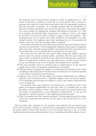
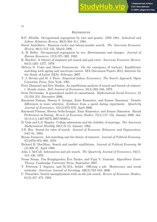
7. 7
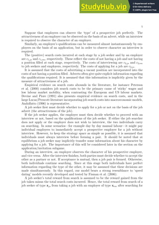
Condition 4: The decisions made by an individual do not depend on the moment
at which the decision is made 4
.
In mathematical terms Conditions 1, 2, 3 are necessary and sufficient conditions to
ensure that when the population use the profile πN
, each individual plays according to
a subgame perfect equilibrium in the appropriately defined application/invitation and
interview subgames.
Since the sets of character measures for job seekers and employers coincide, the most
preferred employees of a type [x1,em, x2,em] employer are job seekers of maximum qualifi-
cations who have character x2,em. The most preferred jobs of a type [x1,js, x2,js] employee
are jobs of maximum attractiveness which have character x2,js. Condition 1 states that
in the interview game a job seeker will always accept his/her most preferred job. Several
labour market studies have found empirical evidence that employers and employees are
happiest with labour market choices they view as similar to themselves in some respects
(eg. labour market type, class, educational level), (Peterson et al., 2000; Beller, 1982;
Albelda, 1981).
Condition 4 states that the Nash equilibrium strategy should be stationary. This reflects
the following facts:
1: An individual starting to search at moment i faces the same problem as one
starting at moment 1.
2: Since the search costs are linear, after searching for i moments and not finding
a job, an individual maximises his/her expected reward from search simply by
maximising the expected reward from future search (i.e. by ignoring previously
incurred costs).
Many strategy profiles may lead to the same pattern of applications, interviews and
employment. For example, suppose that there are three levels of attractiveness and char-
acter, which are the same for both employers and employees. Consider π1, the strategy
profile according to which:
a: job seekers apply to employers of at least the same attractiveness;
b: employers are willing to interview job seekers of at least the same attractiveness;
c: in the interview game, individuals of the two extreme characters accept prospec-
tive job matches of either the same character or of the central character;
d: in the interview game individuals of the central character only accept prospective
partners of the same character.
Under π1 only job seekers and employers of the same attractiveness will proceed to
interview. Pairs are only formed between individuals of the same type.
Suppose π2 differs from π1 in that individuals only apply to or invite for interview
prospective partners of the same attractiveness. The pattern of applications, interviews
and pair formation under these two strategy profiles would be the same.
4Again, this is a restrictive assumption we hope to relax in further work.

8. 8
We might also be interested in Nash equilibrium profiles that satisfy the following
conditions.
Condition 5: In the application/invitation subgame, an employer of type xem is
willing to interview any job seeker of qualifications ≥ tem(xem).
Condition 6: Suppose that if two employers have the same character, then the most
attractive one will be at least as choosy as the other when inviting candidates for
interview.
One might consider analogous conditions for the rules used by job seekers. However,
it seems reasonable that lowly qualified job seekers will not apply for a highly attractive
job, as by doing so they will incur the costs of applying while the employer is expected to
reject them. Since employers only have to decide whether to invite candidates that have
applied to them (i.e. it seems quite possible that the job seeker will ultimately find the
job acceptable), it would seem desirable that they use a threshold rule in this game.
For example, consider an employer of low attractiveness. Under a profile satisfying
Condition 5, she would be willing to interview a job seeker with high qualifications,
although such a job seeker would never accept her in the interviewing game. So, although
Pizza Hut might like a Harvard PhD making pizzas, this is not a realistic match. However,
we expect that under the forces of labour market competition, individuals do not apply
for prospective jobs they are sure to reject in the interview game, as this would be costly
to them. It is simply not worth the Harvard PhD’s time and energy to apply to Pizza
Hut. Hence, in practice Pizza Hut would not have to decide whether to invite such a
candidate for interview for such a post. That is to say, the employer would be indifferent
between the two actions that are purely hypothetically available to her. In this case a
threshold rule is reasonable.
Condition 6 reflects the intuition that employers with highly attractive positions will
be more choosy than employers with a less attractive position.
3. Deriving the Expected Payoffs Under a Given Strategy Profile
Given the strategy profile used by a population, we can define what applications are
made, which pairs of types of individuals proceed to the interview stage, and which pairs
of types of individuals form a job pairing.
From this it is relatively simple to calculate the expected length of search and the
expected number of interview rounds and/or applications of an individual of a given type.
Let p(xjs) be the probability that a job seeker is of type xjs and q(xem) be the probability
that an employer is of type xem.
Let M1(xem; π) be the set of types of employee that an employer of type xem will
interview (i.e. the employee applies to the employer and the employer invites for interview)
under the strategy profile π.
Similarly, let F1(xjs; π) be the set of types of employer that an employee of type xjs
will be interviewed by.

9. 9
Define M2(xem; π) to be the set of types of employee that eventually pair with a employer
of type xem.
Similarly, define F2(xjs; π) to be the set of types of employer that eventually pair with
an employee of type xjs.
Finally, define F0(xjs; π) to be the set of types of employers that a job seeker of type
xjs will apply to.
By definition M2(xem; π) ⊆ M1(xem; π), F2(xjs; π) ⊆ F1(xjs; π) ⊆ F0(xjs; π).
The expected length of search of a job seeker of type xjs, Ljs(xjs; π), is the reciprocal
of the probability of finding an employer with which he will pair at a given stage. The
expected number of interviews of such a job seeker, Djs(xjs; π), is the expected length of
search, times the probability of being interviewed at a given stage. The expected number
of applications, Ajs(xjs; π), can be calculated in an analogous manner.
Hence,
Ljs(xjs; π) =
1
P
xem∈F2(xjs;π) q(xem)
; Djs(xjs; π) =
P
xem∈F1(xjs;π) q(xem)
P
xem∈F2(xjs;π) q(xem)
Ajs(xjs; π) =
P
xem∈F0(xjs;π) q(xem)
P
xem∈F2(xjs;π) q(xem)
.
(1)
Similarly, the expected length of search of an employer of type xem, Lem(xem; π), and the
expected number of interviews held by such an employer, Dem(xem; π), are given by
(2) Lem(xem; π) =
1
P
xjs∈M2(xem;π) p(xjs)
; Dem(xem; π) =
P
xjs∈M1(xem;π) p(xjs)
P
xjs∈M2(xem;π) p(xjs)
.
The expected reward of a type xjs job seeker from accepting a position under the
strategy profile π is the expected reward from taking a job with an employer given that
her type is in the set F2(xjs; π). Hence, the job seeker’s expected total reward from search,
Rjs(xjs; π), is given by
(3) Rjs(xjs; π) =
P
xem∈F2(xjs;π) q(xem)g(x2,js, xem)
P
xem∈F2(xjs;π) q(xem)
− Cjs(xjs; π),
where Cjs(xjs; π) = c1,jsLjs(xjs; π) + c2,jsDjs(xjs; π) + c3,jsAjs(xjs; π) are the expected
search costs of such a job seeker under the strategy profile π. Similarly,
(4)
Rem(xem; π) =
P
xjs∈M2(xem;π) p(xjs)h(xjs, x2,em)
P
xjs∈M2(xem;π) p(xjs)
− c1,emLem(xem; π) − c2,emDem(xem; π).
4. The Interview and Offer/Acceptance Subgames
4.1. The Interview Subgame. Assume that the population are following a strategy
profile π.

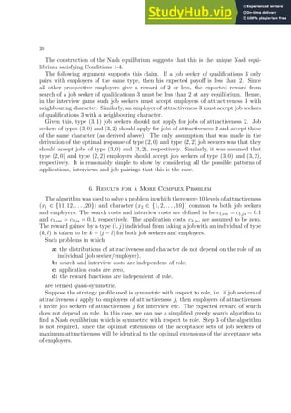
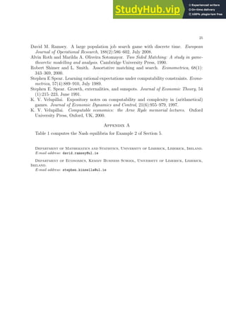
10. 10
The job seeker and employer both have two possible actions: accept the prospective
partner, denoted a, or reject, denoted r.
As argued above, we may assume that these decisions are taken simultaneously.
Also, we ignore the costs already incurred by either individual, including the costs of
the present interview, as they are subtracted from all the payoffs in the matrix, and hence
do not affect the equilibria in this subgame.
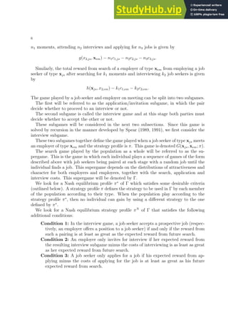
Suppose the job seeker is of type xjs and the employer is of type xem. The payoff matrix
is given by
Employer: a Employer: r
Job Seeker: a
Job Seeker: r
[g(x2,js, xem), h(xjs, x2,em)] [Rjs(xjs; π), Rem(xem; π)]
[Rjs(xjs; π), Rem(xem; π)] [Rjs(xjs; π), Rem(xem; π)]
.
The appropriate Nash equilibrium of this subgame is for the job seeker to accept the job
if and only if g(x2,js, xem) ≥ Rjs(xjs; π) and the employer to accept the job seeker if and
only if h(xjs, x2,em) ≥ Rem(xem; π).
For convenience, we assume that when h(xjs, x2,em) = Rem(xem; π), an employer always
accepts the job seeker (in this case she is indifferent between rejecting and accepting him
for the job). Similarly, if g(x2,js, xem) = Rjs(xjs; π), it is assumed that a job seeker always
accepts an employer.
If a job seeker rejects an employer, then the employer is indifferent between accepting or
rejecting the job seeker. By using the rule given above, an employer will take the optimal
action whenever a job seeker “mistakenly” accepts a job offer.
Under these assumptions, this subgame has a unique Nash equilibrium and value. Let
v(xjs, xem; π) = [vjs(xjs, xem; π), vem(xjs, xem; π)] denote the value of this game, where
vjs(xjs, xem; π) and vem(xjs, xem; π) are the values of the game to the job seeker and
employer, respectively.
We now consider the application/invitation game.
4.2. The Application/Invitation Subgame. Once the interview subgame has been
solved, we may solve the application/invitation subgame and hence the game G(xjs, xem; π).
As before, we assume that the population is following a strategy profile π.
The possible actions of a job seeker are n — do not apply for a job and a — apply for
the job. The possible actions of a potential employee are i - invite for interview and r -
reject an application.
These actions are based on the attractiveness of the prospective partner. As before, we
may ignore the costs that have been previously incurred. Since the order in which the
actions are taken is important, we must consider the extensive form of this game, which
is given below.

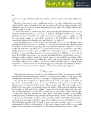
11. 11
✠
❅
❅
❅
❅
❅
❅
❘
Job Seeker: n Job Seeker: a
[Rjs(xjs; π), Rem(xem; π)]
✠
Employer: r
❆
❆
❆
❆
❆
❆
❯
Employer: i
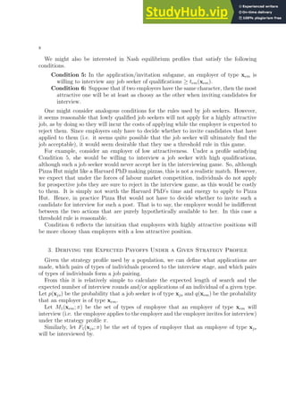
[Rjs(xjs; π) − c3,js, Rem(xem; π)] v(xjs, xem; π) − (c2,js + c3,js, c2,em)
Fig. 1: Extensive form of the application/invitation game.
Here, v(xjs, xem; π) = [vjs(xjs, x1,em; π), vem(x1,js, xjs; π)] denotes the expected value
of the interview game given the strategy profile used by the population, the measures
of attractiveness of the pair, and the fact that an interview followed. In defining these
payoffs, it is assumed that the players are following the appropriate strategy from the
strategy profile π. The calculation of the expected rewards when one individual deviates
from this profile is considered in Section 5.
It should be noted that when a job seeker makes his decision he has no information
regarding the character of an employer.
However, the fact that a job seeker applies for a job may implicitly give the employer
some information regarding his character.
Suppose that under the strategy profile π, the decision of a job seeker of qualifications
x1,js on whether to apply for a job of attractiveness x1,em does not depend on the character
of the job seeker.
The posterior distribution of the character of such a job seeker, given that an application
has been received is simply the marginal distribution of the character of such a job seeker.
In this case, an employer obtains no information on the character of the job seeker, and
we say that the decision of the job seeker is non-revealing (with respect to the character
of the job seeker).
However, if the population has evolved to some equilibrium, the evolutionary process
will have implicitly taught job seekers which type of employers will invite them for inter-
view and which will wish to employ them. This is recursive learning along the lines of
(Velupillai, 2000, Chapter 5), and Spear (1989).
Hence, we assume that job seekers implicitly know the conditional distribution of the
character of the employer given that an interview takes place.
A strategy profile π is said to be non-revealing if the decision of any individual on
whether to apply for a job or invite for interview, as appropriate, is only dependent on
that individual’s attractiveness and not his/her character.
The application/invitation game must be solved by recursion. The employer only has
to make a decision in the case where the job seeker has applied. She should invite for
interview if and only if her expected reward from interviewing is at least as great as the

12. 12
expected reward from future search, i.e.
vem(x1,js, xem; π) − c2,em ≥ Rem(xem; π).
If no employer of the attractiveness observed wishes to invite the job seeker for interview,
then the job seeker should not apply.
Otherwise, the job seeker should apply if
r(x1,js, x1,em; π)[vjs(xjs, x1,em; π)−c2,js]+(1−r(x1,js, x1,em; π)Rjs(xjs; π)−c3,js ≥ Rjs(xjs; π),
where r(x1,js, x1,em; π) is the probability that a randomly chosen employer of attractiveness
x1,em wishes to invite a job seeker of qualifications x1,js for interview.
We now present an algorithm to solve such a game, as an algorithmic game in the
tradition of Velupillai (1997); Nisam et al. (2007).
5. An Algorithm to Derive a Subgame Perfect Equilibrium
The algorithm proposed to find a Nash equilibrium of the game satisfying Conditions
1-4 starts by assuming that:
1: job seekers of the highest level of attractiveness will only apply for jobs of the
highest level of attractiveness and they will be invited for interview by such em-
ployers.
2: job seekers and employers of maximum attractiveness only form pairs with others
of the same character (remember that it is assumed that the sets of possible
characters for these groups coincide).
It should be noted that this will be part of a Nash equilibrium profile when the search
and interviewing costs are sufficiently small. This follows from the following argument:
For sufficiently small costs, job seekers of maximum qualifications only wish to take a job
with their preferred type of ‘partner’ (i.e. jobs of maximum attractiveness with the same
character). Similarly, employers are only willing to offer jobs of maximum attractiveness
to job seekers of maximum attractiveness and the same character.
It should be noted that if at equilibrium a job seeker of type [i, j] is willing to apply
for a job of attractiveness k, then he must be willing to accept a job of type [k, j] in the
interview game. This is due to the fact that a job seeker of type [i, j] would not apply for
such a job, if he were not willing to take any job of attractiveness k, and type [k, j] jobs
are the most preferred jobs in this group. Similarly, if an employer of type [i, j] is willing
to invite a job seeker of attractiveness k for interview, he must be willing to offer a job
to a job seeker of type [k, j].
We can calculate the expected rewards of individuals of maximum attractiveness under
the initial strategy profile. We then iteratively improve the payoffs of job seekers and em-
ployers of maximum qualifications by changing the patterns of applications, interviewing
and job pairings as follows:
1: At each stage extend the set of acceptable jobs of all job seekers of maximum
qualifications by increasing the acceptable difference in character by 1 or decreasing

13. 13
the minimum level of attractiveness required to make an application by 1. The
choice of direction in which to extend the set of acceptable jobs is chosen to
maximise the expected reward from search given that the appropriate employers
find the job seeker acceptable. It is initially assumed that the distribution of
character of either an employer who invites for interview or job seeker who applies
for a job is simply the appropriate marginal distribution of character (i.e. that
if an employer of relatively high attractiveness is willing to invite a job seeker
for interview, then the job seeker is willing to apply to such an employer). This
assumption may not be correct and is later checked by the algorithm. It is then
checked whether the employers gain from increasing the set of acceptable job
seekers in this way. If so the strategy profile is updated.
It should be noted that if a job seeker can increase his expected reward in both of
the ways described above, but the appropriate employers do not gain by employing
such a job seeker, then the strategy profile is not updated and the second direction
of extending the set of acceptable jobs is considered in the same way.
We start each step with the type of job seeker having the highest expected
reward under the present strategy profile, and finish with the type having the
least reward. It should be noted that when the level of attractiveness required to
induce an application is reduced, any type which gives a reward at least as great
as any type already in the set of acceptable jobs should also be included.
2: The step described above is repeated until no improvements in the expected
payoffs of job seekers of maximum qualifications are possible.
3: This procedure is repeated for employers of maximum attractiveness (some of the
calculations will already have been done when extending the sets of jobs acceptable
to job seekers of maximum attractiveness).
4: Suppose some, but not all, job seekers of maximum qualifications are willing to
apply for a job of attractiveness x1. Similarly, suppose, some, but not all, employ-
ers of maximum attractiveness are willing to invite a job seeker of attractiveness
x2 for an interview.
It is possible that some employers of attractiveness x1 should not invite a job
seeker of maximum qualifications for interview, since it is possible that no such
job seeker would be willing to form a pair. Steps 1 and 2 are repeated given that
job seekers of qualifications x1 and employers of attractiveness x2 now use the
appropriate “optimal response” in the application/invitation game.
5: Step 4 is repeated until the “optimal responses” of both employers and job seekers
of less than maximum attractiveness are the same at the end of Step 4 as at the
beginning.
This procedure then continues for job searchers and employers of successively lower
levels of attractiveness. Initially, it assumed that no applications, interviews and pairings
are made outside of those that already occur in the profile built up so far. It is then
checked whether the most preferred partner not yet considered should be added to the set

14. 14
of acceptable jobs or acceptable employees, as appropriate. The algorithm then continues
as before. Since the algorithm attempts to maximise the expected reward of an individ-
ual, given the behaviour of individuals of relatively higher attractiveness, the pattern of
applications, interviews and job pairings that results from this procedure will, in general,
be very similar to the pattern of applications, interviews and job pairings that results
from a Nash equilibrium strategy profile.
It should also be noted that the “strategy profiles” considered in this algorithm are not
fully defined strategy profiles. Only the pattern of applications, interviews and job pairings
are defined. Once the algorithm has converged, we use the policy iteration algorithm to
check whether the proposed pattern corresponds to a Nash equilibrium of the required
form and, if so, fully define the strategy profile.
We illustrate this algorithm with an example.
5.1. Example. Suppose that among both employers and job seekers there are 2 levels
of attractiveness, X1 ∈ {2, 3}, and three levels of character X2 ∈ {0, 1, 2}. Each of the
six possible types are equally likely. The search costs for both job seekers and employers,
denoted c1, are 0.3. The costs of interviewing for an employer, c2,em, are 0.25. The costs
of applying for a job are c3,js = 0.1 and the costs of a job seeker going for an interview
are c2,js = 0.15.
The reward obtained by a type [i, j] individual forming a job pairing with a type [k, l]
individual is assumed to be k − |j − l| (for both job seekers and employers).
We initially assume that job seekers of maximum attractiveness only apply for jobs
of maximum attractiveness and only accept jobs with the same character. Employers of
maximum attractiveness only invite job seekers of maximum attractiveness for interview
and only offer jobs to job seekers of the same character. It follows that the expected
length of search of such individuals is 6 and the number of interviews (and applications)
is 3. Since a job seeker’s costs for applying and going to an interview are equal to the
employer’s interview costs, the expected reward gained under such a profile (labelled π0) is
independent of an individual’s role (employer or job seeker). It follows that for y = 0, 1, 2
Rem([3, y]; π0) = Rjs([3, y]; π0) = 3 − 0.3 × 6 − 0.25 × 3 = 0.45.
We now consider expanding the set of types of job acceptable to a job seeker of maximum
attractiveness.
From the form of the payoff function, and the distribution of types, it is of greater
benefit for such a job seeker to accept jobs of attractiveness 3 with a neighbouring level of
character (such a strategy profile will be denoted π1), rather than jobs of attractiveness
2 with the same character.
This follows from the fact that the reward from taking either type of job would be the
same, but only applying for jobs of attractiveness 3 does not increase the expected costs
incurred in applications/interviews.

15. 15
The reward obtained by any job seeker of maximum attractiveness, is greater under a
strategy profile of the form π1 (given the relevant employers find the job seekers acceptable)
than the expected reward under π0.
From the ”symmetry” of the problem, the newly acceptable employers would also find
the job seekers acceptable. Hence, the sets of jobs acceptable to job seekers of attractive-
ness 3 should be extended, along with the sets of job seekers acceptable to employers of
attractiveness 3. After such an extension
1: Type (3, 0) individuals (both job seekers and employers) pair with type (3, 0) and
(3, 1) individuals.
2: Type (3, 1) individuals pair with type (3, 0), (3, 1) and (3, 2) individuals.
3: Type (3, 2) individuals pair with type (3, 1) and (3, 2) individuals.
The expected payoffs of individuals of attractiveness 3 under such a profile π1 are given
by
R•([3, 0]; π1) = R•([3, 2]; π1) = =
1
2
(2 + 3) − 0.3 × 3 − 0.25 ×
3
2
= 1.225
R•([3, 1]; π1) =
1
3
(2 + 3 + 2) − 0.3 × 2 − 0.25 ≈ 1.4833,
where • stands for either js or em.
We now check whether a type (3, 1) job seeker can gain by accepting type (2, 1) jobs.
Note that a type (3, 0) job seeker cannot gain by accepting a type (3, 2) job, as the reward
obtained from taking such a job is less than Rjs([3, 0]; π1). Hence, we must only check
whether type (3, 0) job seekers can gain by accepting type (2, 0) jobs. If so, by symmetry
type (3, 2) job seekers can gain by accepting type (2, 2) jobs. Under such a profile, π2,
job seekers of attractiveness 3 would be willing to apply for any prospective job. Since
employers of attractiveness 2 have not yet become acceptable to any job seeker, it is clear
that in this case such employers increase their expected reward from search by accepting
the job seekers under consideration. Hence, under π2 job seekers of type [3, 0] apply for
all positions, are interviewed for all positions and pair with employers of type (3, 0), (3, 1)
and (2, 0). Hence, the expected length of search, as well as the expected number of
both applications and interviews, is equal to 2. Job seekers of type [3, 1] apply for any
position, are always interviewed and pair with employers of type (2, 1), (3, 0), (3, 1) and
(3, 2). The expected length of search, as well as the expected number of both interviews
and applications, is equal to 3
2
. Using symmetry with respect to the central character,
the expected rewards of job seekers of attractiveness 3 under π2 are given by
Rjs([3, 0]; π2) = Rjs([3, 2]; π2) =
1
3
(2 + 3 + 2) − 0.3 × 2 − 0.25 × 2 ≈ 1.2333
Rjs([3, 1]; π2) =
1
4
(2 + 3 + 2 + 2) − 0.3 ×
3
2
− 0.25 ×
3
2
≈ 1.425.
Hence, type (3, 0) job seekers should accept type (2, 0) jobs, but type (3, 1) job seekers
should not accept type (2, 1) jobs. Let π3 be the corresponding profile.

16. 16
Since the expected payoffs of job seekers of attractiveness 3 are greater than can be
obtained by accepting any type of job not yet considered, Steps 1 and 2 are concluded.
We now consider extending the sets of job seekers acceptable to employers. From the
earlier calculations employers of attractiveness 3 should accept job seekers of attractiveness
3 with a neighbouring character. Using the symmetry of the problem, it follows that type
(3, 0) employers should accept type (2, 0) job seekers and type (3, 2) employers should
accept type (2, 2) job seekers.
We now consider whether job seekers of attractiveness 2 should be willing to apply for
jobs of attractiveness 3. Since job seekers of attractiveness 2 are only invited for interview
by employers of type (3, 0) and (3, 2) and such employers will not offer a job to a job
seeker of type (2, 1), it follows that job seekers of type (2, 1) should not apply for jobs of
attractiveness 3. Similarly, an employer of type (2, 1) should not invite an individual of
attractiveness 3 for an interview.
Denote this new profile by π4. Under such a profile, when an employer of attractiveness
3 invites a job seeker of attractiveness 2 for an interview, the conditional distribution of
the character of either is as follows: 0 with probability 1
2
and 2 with probability 1
2
.
Now consider the best response of employers of attractiveness 3. Employers of type
(3, 1) should not accept job seekers of type (2, 0) and (2, 2) and thus not invite job seekers
of attractiveness 2 for interview. Employers of type (3, 0) should still invite job seekers
of attractiveness 2 for an interview, as it is more likely under π4 than under π3 that the
job seeker will be of the only acceptable corresponding type. Similarly, the best response
of job seekers of attractiveness 3 is as derived in Step 1. Under π4, job seekers of type
(3, 0) apply for all jobs, are not interviewed only by type (2, 1) employers and pair with
employers of type (3, 0), (3, 1) and (2, 0). Employers of type (3, 0) will interview all job
seekers except those of type (2, 1) and pair with job seekers of type (3, 0), (3, 1) and (2, 0).
We have
Rem([3, 1]; π4) = Rjs([3, 1]; π4) = Rem([3, 1]; π1) ≈ 1.4833
Rem([3, 0]; π4) = Rem([3, 2]; π4) =
1
3
(2 + 3 + 2) − 0.3 × 2 − 0.25 ×
5
3
≈ 1.3167.
Rjs([3, 0]; π4) = Rjs([3, 2]; π4) =
1
3
(2 + 3 + 2) − 0.3 × 2 − 0.15 ×
5
3
− 0.1 × 2 ≈ 1.2833.
We now consider extending the sets of jobs acceptable to job seekers of attractiveness
2. Under π4, job seekers of type (2, 0) apply for jobs of attractiveness 3, are interviewed
by employers of type (3, 0) and (3, 2) and pair with employers of type (3, 0). As of yet,
job seekers of type (2, 1) do not apply for any job. Using symmetry with respect to the
central character, we obtain
Rjs([2, 0]; π4) = Rjs([2, 2]; π4) = 3 − 0.3 × 6 − 0.15 × 2 − 0.1 × 3 = 0.6.

17. 17
Under π4, employers of type (2, 0) interview job seekers of type (3, 0) and (3, 2) and form
pairs with job seekers of type (3, 0). It follows that
Rem([2, 0]; π4) = Rem([2, 2]; π4) = 3 − 0.3 × 6 − 0.25 × 2 = 0.7.
We first consider extending the sets of acceptable jobs to include jobs of the same type
as the job seeker. These are the most preferable jobs of those that have not yet been
considered. Under the resulting strategy profile, π5, job seekers of type (2, 0) apply for all
jobs, are interviewed by all employers except those of type (3, 1) and pair with employers
of type (2, 0) and (3, 0). Job seekers of type (2, 1) only apply for jobs of attractiveness
2, are interviewed for all such positions and pair with employers of type (2, 1). It follows
that
Rjs([2, 0]; π5) = Rjs([2, 2]; π5) =
1
2
(2 + 3) − 0.3 × 3 − 0.15 × 52 − 0.1 × 3 = 0.925
Rjs([2, 1]; π5) = 2 − 0.3 × 6 − 0.25 × 3 = −0.55
Since type (2, 1) employers do not yet accept any type of job seeker, they improve their
expected payoff by accepting type (2, 1) job seekers. By accepting type (2, 0) job seekers,
type (2, 0) employers now interview all job seekers except those of type (3, 1) and pair
with job seekers of type (2, 0) and type (3, 0). Their expected reward from search is given
by
Rem([2, 0]; π5) = Rem([2, 2]; π5) =
1
2
(2 + 3) − 0.3 × 3 − 0.25 ×
5
2
= 0.975.
Hence, the payoffs of employers increase and so the profile is updated to π5.
Since the expected payoffs of all job seekers of attractiveness 2 under π5 are less than
that gained from pairing with an employer of attractiveness 2 with a neighbouring level of
character, the sets of jobs acceptable to them should be extended. Denote the resulting
profile by π6. We have
Rjs([2, 0]; π6) = Rjs([2, 2]; π6) =
1
3
(2 + 3 + 1) − 0.3 × 2 − 0.15 ×
5
3
− 0.1 × 2 = 0.95
Rjs([2, 1]; π6) =
1
3
(1 + 2 + 1) − 0.3 × 2 − 0.25 ≈ 0.4833.
Under such an extension of the strategy profile, type (2, 0) employers interview all job
seekers except those of type (3, 1) and pair with those of type (2, 0), (3, 0) or (2, 1). Type
(2, 1) employers only interview job seekers of attractiveness 2 and will pair with all such
job seekers. It follows that
Rem([2, 0]; π6) = Rem([2, 2]; π6) =
1
3
(2 + 3 + 1) − 0.3 × 2 − 0.25 ×
5
3
= 0.9833
Rem([2, 1]; π6) =
1
3
(1 + 2 + 1) − 0.3 × 2 − 0.25 ≈ 0.4833.
The expected payoffs of employers of attractiveness 2 has increased and thus we update
the strategy profile to π6.

18. 18
Extending the sets of acceptable jobs will not increase the expected reward of any of
these job searchers. Similarly, extending the sets of acceptable employees will not increase
the expected reward of any of the employers.
It follows that π6 is our candidate for a profile of applications, interviews and job pair
formation which corresponds to a Nash equilibrium satisfying Conditions 1-4.
We now use policy iteration to check whether this profile corresponds to a strategy
profile which satisfies the appropriate criteria. First, we consider the interview game.
Each individual (of either role) should accept a prospective job when the reward obtained
from such a pairing is at least as great as the expected reward from future search. It
follows that
1: Type (3, 0) individuals should pair with individuals of type (3, 0), (3, 1) or (2, 0).
2: Type (3, 1) individuals should pair with individuals of type (3, 0), (3, 1), (3, 2) or
(2, 1).
3: Type (3, 2) individuals should pair with individuals of type (3, 1), (3, 2) or (2, 2).
4: Type (2, 0) individuals should pair with individuals of type (2, 0), (2, 1), (3, 0),
(3, 1) or (3, 2). However, acceptance is not mutual in the final two cases.
5: Type (2, 1) individuals should pair with any prospective job, but acceptance is
not mutual when the prospective job is of type (3, 0) or (3, 2).
6: Type (2, 2) individuals should pair with individuals of type (2, 1), (2, 2), (3, 2),
(3, 1) or (3, 0). However, acceptance is not mutual in the final two cases.
We now consider the application/invitation game. This game is solved by recursion
starting with the calculation of the optimal response of an employer to a job seeker of
qualifications i who has applied for a post, where i ∈ {2, 3}.
If under any strategy profile π an employer of attractiveness j invites some job seekers
of qualifications i for an interview, then it is assumed that the distribution of the character
of the job seeker comes from the conditional distribution of character given the invitation
for an interview. An analogous assumption is made with regard to the distribution of the
character of an employer who has invited a job seeker for an interview.
Suppose no job seeker of qualifications i is willing to apply to an employer of attrac-
tiveness j under π. In order to determine the appropriate response of an employer, it is
assumed that the distribution of the character of the job seeker is simply the marginal
distribution of the character of job seekers (i.e. the probability of an individual making a
“mistake” is o(1) and independent of his/her type). Analogous assumptions are made in
the calculation of whether a job seeker should be willing to apply or not.
First consider a type (3, 0) employer who has been applied to by a job seeker of qualifi-
cations 3. Since all job seekers of qualifications 3 are willing to apply to such an employer,
the expected reward from such an interview satisfies
vem([3, 0], 3) =
1
3
[3 + 2 + Rem([3, 0]; π6)] − 0.25 Rem([3, 0]; π6).
Hence, a type (3, 0) employer should invite for interview.
Now suppose a type (3, 0) employer is applied to by a job seeker of qualifications 2.

19. 19
Such a job seeker is of type (2, 0) with probability 1
2
, otherwise he is of type (2, 2). It
follows that the expected reward from inviting such a job seeker for interview is
vem([3, 0], 2) =
1
2
[2 + Rem([3, 0]; π6)] − 0.25 Rem([3, 0]; π6).
Hence, a type (3, 0) employer should invite for interview. It follows from the symmetry
with respect to character that type (3, 2) employers should invite any job seeker for
interview.
Using a similar procedure, it can be shown that type (3, 1) employers should only
invite job seekers of qualifications 3 for interview. Type (2, 0) and type (2, 2) employers
should invite any job seeker and type (2, 1) employers should only invite job seekers of
qualifications 2. Note that since no job seeker of qualifications 3 who is prepared to apply
to an employer of qualifications 2 will pair with an employer of type (2, 1), such employers
should reject the application of a job seeker of qualifications 3.
Now consider the optimal action of a job seeker given the response of an employer
defined above. Any employer of attractiveness 3 will invite a job seeker of qualifications
3 for interview. Hence, by applying to such an employer, a job seeker of type (3, 0) has
an expected reward of 1
3
[3 + 2 + Rjs([3, 0]; π6)] − 0.25. This reward is Rjs([3, 0]; π6).
Hence, a type (3, 0) job seeker should apply to an employer of attractiveness 3. Similarly,
job seekers of type (3, 1) and type (3, 2) should apply to an employer of attractiveness 3.
Now consider whether a job seeker of type (3, 0) should apply to an employer of at-
tractiveness 2. Employers of type (2, 1) will reject such an application, only application
costs are incurred and the future expected reward of the job seeker (including these
costs) is Rjs([3, 0]; π6) − c3,js. Employers of type (2, 0) and (2, 2) will invite such a job
seeker for interview, and the future expected rewards of the job seeker in these cases are
2 − c2,js − c3,js = 1.75 and Rjs([3, 0]; π6) − c2,js − c3,js, respectively. It follows that the
expected reward obtained from applying in this case is 1
3
[1.75 + 2Rjs([3, 0]; π6) − 0.35] ≈
1.3222 Rjs([3, 0]; π6).
Hence, a job seeker of type (3, 0) should apply to an employer of attractiveness 2.
Arguing similarly, job seekers of type (3, 2) should apply to employers of attractiveness 2,
but job seekers of type (3, 1) should not.
In a similar way, it can be shown that job seekers of type (2, 0) or (2, 2) should apply to
any employer and job seekers of type (2, 1) should only apply to employers of attractiveness
2.
The strategy constructed in this way defines a subgame perfect equilibrium in the
game G(xjs, xem; π6). Also, it can be seen that this strategy leads to the same pattern of
applications, interviews and job pairings as under π6. One interesting aspect of the full
description of this strategy profile is that (3, 1) individuals would pair with type (2, 1)
individuals in the interview game, but the marginal gain of such a pairing is not large
enough to ever justify the costs of a type (3, 1) job seeker applying to an employer of
attractiveness 2, or a type (3, 1) employer inviting a job seeker of attractiveness 2 for an
interview.

20. 20
The construction of the Nash equilibrium suggests that this is the unique Nash equi-
librium satisfying Conditions 1-4.
The following argument supports this claim. If a job seeker of qualifications 3 only
pairs with employers of the same type, then his expected payoff is less than 2. Since
all other prospective employers give a reward of 2 or less, the expected reward from
search of a job seeker of qualifications 3 must be less than 2 at any equilibrium. Hence,
in the interview game such job seekers must accept employers of attractiveness 3 with
neighbouring character. Similarly, an employer of attractiveness 3 must accept job seekers
of qualifications 3 with a neighbouring character.
Given this, type (3, 1) job seekers should not apply for jobs of attractiveness 2. Job
seekers of types (3, 0) and (3, 2) should apply for jobs of attractiveness 2 and accept those
of the same character (as derived above). The only assumption that was made in the
derivation of the optimal response of type (2, 0) and type (2, 2) job seekers was that they
should accept jobs of type (3, 0) and (3, 2), respectively. Similarly, it was assumed that
type (2, 0) and type (2, 2) employers should accept job seekers of type (3, 0) and (3, 2),
respectively. It is reasonably simple to show by considering all the possible patterns of
applications, interviews and job pairings that this is the case.
6. Results for a More Complex Problem
The algorithm was used to solve a problem in which there were 10 levels of attractiveness
(x1 ∈ {11, 12, . . . , 20}) and character (x2 ∈ {1, 2, . . . , 10}) common to both job seekers
and employers. The search costs and interview costs are defined to be c1,em = c1,js = 0.1
and c2,em = c2,js = 0.1, respectively. The application costs, c3,js, are assumed to be zero.
The reward gained by a type (i, j) individual from taking a job with an individual of type
(k, l) is taken to be k − |j − l| for both job seekers and employers.
Such problems in which
a: the distributions of attractiveness and character do not depend on the role of an
individual (job seeker/employer),
b: search and interview costs are independent of role,
c: application costs are zero,
d: the reward functions are independent of role.
are termed quasi-symmetric.
Suppose the strategy profile used is symmetric with respect to role, i.e. if job seekers of
attractiveness i apply to employers of attractiveness j, then employers of attractiveness
i invite job seekers of attractiveness j for interview etc. The expected reward of search
does not depend on role. In this case, we can use a simplified greedy search algorithm to
find a Nash equilibrium which is symmetric with respect to role. Step 3 of the algorithm
is not required, since the optimal extensions of the acceptance sets of job seekers of
maximum attractiveness will be identical to the optimal extensions of the acceptance sets
of employers.

21. 21
This algorithm was used to derive a candidate for the pattern of applications, interviews
and job pairings observed at a Nash equilibrium satisfying Conditions 1-4. It was assumed
that this pattern was symmetric with respect to character (i.e. by taking 10 − j rather
than j to be the character of an individual, the pattern remained the same). Analysis of
the interview and application/invitation subgames confirmed that the proposed pattern
corresponded to such a Nash equilibrium. It was assumed that job seekers were only
prepared to apply for a job of attractiveness i, if there existed employers of attractiveness
j with which he would eventually form a pair. The pattern of job pairings proposed by
the algorithm is described by Table 1 in the appendix.
It should be noted that there are other Nash equilibria which satisfy Conditions 1-4.
For example, at the equilibrium presented above no job seeker of qualifications 20 is
willing to apply for jobs of attractiveness 17. It can be easily checked that under the
hypothesis that all employers of attractiveness 17 are willing to interview prospective job
seeker of qualifications 20, then it would not pay a type (20, 1) or (20, 10) job seeker
to be willing to apply for such a position (these two types of job seeker are the only
types that might benefit from such interview, as the expected payoff of the remaining job
seekers of maximum qualifications are all greater than 17). In the same way, it would
not pay type (20, 1) or (20, 10) job seekers to apply for jobs of attractiveness 17 when all
such prospective employers are unwilling to interview. This follows from the assumption
that the probability of making a “mistake” is independent of the type of an individual.
However, suppose employers of type (17, 1) and (17, 10) are willing to interview job seekers
of qualifications 20, while other employers of attractiveness 17 are unwilling. In this case,
it can be shown that job seekers of type (20, 1) and type (20, 10) should be willing to
apply for jobs of attractiveness 17 and then accept the job if it is of the same character
as the applicant.
It was assumed that the equilibrium is symmetric with respect to both role and charac-
ter, but there are equilibria which do not satisfy this criterion. For example, suppose only
type (17, 1) job seekers and no other job seekers of attractiveness 17 are willing to apply
for jobs of attractiveness 20. It will be optimal for employers of type (20, 1) to invite job
seekers of qualifications 17 for interview, but not for employers of type (20, 10).
Further equilibria can be found by changing the set of job seekers of qualifications 18
who are willing to apply for jobs of attractiveness 20. At the equilibrium described above,
some employers of attractiveness 20 are willing to interview job seekers of qualifications
18, but none pair with a job seeker of type (18, 4). It follows that job seekers of type
(18, 4) should not be willing to apply for jobs of attractiveness 20. Employers of type
(20, 3) should be willing to interview job seekers of qualifications 18, since the conditional
probability of such a job seeker being of type (18, 3) given that interview follows is greater
than the marginal probability of the job seeker being of character 3. However, suppose
that job seekers of type (18, 4) rather than of type (18, 3) are willing to apply for jobs of
attractiveness 20. In this case, employers of type (20, 4) should be willing to interview
job seekers of qualifications 18 and pair with those of type (18, 4). On the other hand,

22. 22
employers of type (20, 3) should not be willing to interview job seekers of qualifications
18.
In each of these cases, a new equilibrium may be derived by making the appropriate
change in the pattern of applications, interviews and job pairings observed among indi-
viduals of maximum attractiveness and calculating the pattern for individuals of lower
attractiveness as before.
It seems that there is a very large set of Nash equilibria satisfying Conditions 1-4 for
the problem investigated and the problem of deriving all of them would seem to be very
difficult. However, from the form of the game it seems that all these equilibria would
be qualitatively similar in terms of the choosiness of the individuals and the level of
association between the attractiveness and characters of partners.
One interesting aspect of the equilibrium presented here is that the choices of the
individuals of attractiveness of 17 or lower in this game are non-revealing. Job seekers of
such attractiveness are willing to apply for jobs whose attractiveness is not more than one
level from their own. Since the costs of application are zero, it follows that a job seeker
of attractiveness 16 or less would be indifferent to applying for a job of attractiveness at
least two levels greater than themselves, as such an employer would always reject such an
offer. It would be interesting to see whether simulation of the evolution of such strategy
profiles in such a scenario would lead to job seekers of low qualifications being willing
to apply for jobs of high attractiveness (i.e. would their strategies satisfy the analogous
conditions to Conditions 5 and 6). The results of the evolution of such a system would
depend on the relative costs and benefits of applying for such jobs away from equilibrium.
Future work will concentrate on large scale simulation studies of such games.
7. Conclusion
This paper has presented a model of mutual job search where both common and ho-
motypic preferences are taken into account. An algorithm for finding a Nash equilibrium
satisfying various criteria based on the concept of subgame perfection was described.
The use of this combination of preferences would seem to be logical in relation to
job choice. Although there is no perfect correlation in individuals’ assessment of the
attractiveness of members of the opposite labour market type, there is normally a very
high level of agreement, particularly among job seekers. This approach has been used,
for example, by Gale and Shapley (1962). Using such an approach individuals have their
own personal ranking of the desirability of members of the opposite labour market type.
The approach used here would seem to be a good compromise between the approaches
used in matching and the assumptions of common preferences. These ”mixed” preferences
seem to be both reasonably tractable within the framework of searching for a job within a
relatively large population and allow a general enough framework to model the preferences
of individuals reasonably well (although it would seem that modelling character as a one-
dimensional variable is rather simplistic). By using a larger number of types, we could
approximate continuous distributions of qualifications and character Ramsey (2008).

23. 23
For simplicity it was assumed that individuals know their own qualifications and char-
acter, whereas in practice they may have to learn about these measures over time.
Also, individuals are able to measure attractiveness and character perfectly, although
at some cost. It would be interesting to consider different ways in which information is
gained during the search process. For example, some information about the character of
a prospective labour market match may be readily available. Hence, an improved model
would allow some information to be gained on both the attractiveness and character of a
prospective partner at each stage of the decision process.
In terms of the evolution of such procedures, it is assumed that the basic framework
is given, i.e. the model assumes that the various search, application and interview costs
are given. It should be noted that labour markets may benefit from the interview process
i.e. employers might find employees of different qualifications to those stated in the
advertisement, but still useful to the company.
However, this model cannot explain why such a system has evolved, only the evolution
of decisions within this framework. Individuals may lower their search costs by joining
some internet or social group. Such methods can also lead to biasing the conditional
distribution of the character of a prospective job in a searcher’s favour. It might be
that interviewing costs are dependent on the types of the two individuals involved. For
example, two individuals of highly different characters might incur low interview costs, as
they realise very quickly that they are not well matched.
Also, the ability to incur interview costs may well transfer information regarding the
attractiveness and/or character of a job seeker. Hence, it may be more costly to be
interviewed by highly attractive employers, since they would have strong preferences for
high quality (i.e. attractive) job seekers.
As it seems there may be a large number of Nash equilibria satisfying the required
conditions, it would be of interest to carry out simulations of how job choice strategies
evolve within such a framework using replicator dynamics.
Also, it would be useful to investigate how the payoff functions, together with the
relative costs of searching and interviewing, affect the importance of qualifications and
character in the decision process. It should be noted that using qualifications as an initial
filter in the decision process will lead to qualifications becoming relatively more important
than character, especially if the costs of interviewing are relatively high. If we consider the
simple example given in Section 5.1, individuals of type (3, 1) do not pair with prospective
jobs of type (2, 1), although they are just as good pairings as either jobs of type (3, 0) or
(3, 2). It is intended that a future paper will investigate these issues in more detail.
Finally, the algorithm presented starts with each individual being choosy. We could
define a similar algorithm in which each individual starts by being completely non-choosy.
This algorithm would proceed by successively removing types that an individual of max-
imum attractiveness should clearly not pair with until no improvement can be made by
removing further types from this set. This would be repeated for successively less attrac-
tive individuals in the labour market.

24. 24
References
R.P. Albelda. Occupational segregation by race and gender: 1958–1981. Industrial and
Labour Relations Review, 39(3):404–411, 1981.
David Andolfatto. Business cycles and labour-market search. The American Economic
Review, 86(1):112–132, March 1996.
A. H. Beller. Occupational segregation by sex: Determinants and changes. Journal of
Human Resources, 17(3):371–392, 1982.
K. Burdett. A ttheory of employee job search and quit rates. American Economic Review,
84(5):1261–1277, 1978.
Melvyn G. Coles and Marco Francesconi. On the emergence of toyboys: Equilibrium
matching with ageing and uncertain careers. IZA Discussion Papers 2612, Institute for
the Study of Labor (IZA), February 2007.
T. J. Devine and M. J. Piore. Empirical Labour Economics: The Search Approach. Open
University Press, New York, 1991.
Peter Diamond and Eric Maskin. An equilibrium analysis of search and breach of contract
i: Steady states. Bell Journal of Economics, 10(1):282–316, 1979.
Scott Drewlanka. A generalized model of commitment. Mathematical Social Sciences, 52
(3):233–251, December 2006.
Raymond Fisman, Sheena S. Iyengar, Emir Kamenica, and Itamar Simonson. Gender
differences in mate selection: Evidence from a speed dating experiment. Quarterly
Journal of Economics, 121(2):673–679, April 2006.
Raymond Fisman, Sheena Sethi-Iyengar, Emir Kamenica, and Itamar Simonson. Racial
Preferences in Dating. Review of Economic Studies, 75(1):117–132, January 2008. doi:
10.1111/j.1467-937X.2007.00465.x.
D. Gale and L.S. Shapley. College admissions and the stability of marriage. The American
Mathematical Monthly, 69(1):9–15, January 1962.
J.D. Hey. Search for rules of search. Journal of Economic Behaviour and Organisation,
3:65–81, 1982.
Boyan Jovanovic. Job matching and the theory of turnover. Journal of Political Economy,
87(1979):972–990, 1979.
Richard D. MacMinn. Search and market equilibrium. Journal of Political Economy, 88
(2):308–27, April 1980.
John J. McCall. Information and job search. The Quarterly Journal of Economics, 84(1):
113–126, 1970.
Noam Nisam, Tim Roughgarden, Éva Tardos, and Vijay V. Vazirani. Algorithmic Game
Theory. Cambridge University Press, September 2007.
T. Peterson, I. Saporta, and M.-D.L. Seidel. Offering a job: Meritocracy and social
networks. American Journal of Sociology, 106(3):763–816, 2000.
C. Pissarides. Search unemployment with on-the-job search. Review of Economic Studies,
61(3):457–475, 1994.

25. 25
David M. Ramsey. A large population job search game with discrete time. European
Journal of Operational Research, 188(2):586–602, July 2008.
Alvin Roth and Marilda A. Oliveira Sotomayor. Two Sided Matching: A study in game-
theoretic modelling and analysis. Cambridge University Press, 1990.
Robert Shimer and L. Smith. Assortative matching and search. Econometrica, 68(1):
343–369, 2000.
Stephen E Spear. Learning rational expectations under computability constraints. Econo-
metrica, 57(4):889–910, July 1989.
Stephen E. Spear. Growth, externalities, and sunspots. Journal of Economic Theory, 54
(1):215–223, June 1991.
K. V. Velupillai. Expository notes on computability and complexity in (arithmetical)
games. Journal of Economic Dynamics and Control, 21(6):955–979, 1997.
K. V. Velupillai. Computable economics: the Arne Ryde memorial lectures. Oxford
University Press, Oxford, UK, 2000.
Appendix A
Table 1 computes the Nash equilibria for Example 2 of Section 5.
Department of Mathematics and Statistics, University of Limerick, Limerick, Ireland.
E-mail address: david.ramsey@ul.ie
Department of Economics, Kemmy Business School, University of Limerick, Limerick,
Ireland.
E-mail address: stephen.kinsella@ul.ie

26. 26
Type Pairs with Reward
(20, j), j = 4, 5 (20, j ± 2), (20, j ± 1), (20, j), (19, j ± 1), (19, j) 17.1250
(20, j), j = 3 (20, j ± 2), (20, j ± 1), (20, j), (19, j ± 1), (19, j), (18, 3) 17.1556
(20, j), j = 2 (20, 4), (20, j ± 1), (20, j), (19, j ± 1), (19, j), (18, 2) 17.0500
(20, 1) (20, 1), (20, 2), (20, 3), (19, 1), (19, 2), (18, 1), (18, 2) 16.6750
(19, j), j = 4, 5 (20, j ± 1), (20, j), (19, j ± 2), (19, j ± 1), (19, j), (18, j ± 1), (18, j) 16.9091
(19, j), j = 3 (20, 1), (20, j ± 1), (20, j), (19, j ± 2), 17.0000
(19, j ± 1), (19, j), (18, j ± 1), (18, j)
(19, j), j = 2 (20, j ± 1), (20, j), (19, j ± 1), (19, j), (19, 4)(18, j ± 1), (18, j) 16.9000
(19, 1) (20, 1), (20, 2), (19, 1), (19, 2), (19, 3), (18, 1), (18, 2) 16.4286
(18, j), j = 4, 5 (19, j ± 1), (19, j), (18, j ± 1), (18, j), (18, j + 2)(17, j ± 1), (17, j) 15.9000
(18, j), j = 3 (20, j), (19, j ± 1), (19, j), (18, j ± 1), (18, j) 16.3429
(18, j), j = 2 (20, 1), (20, 2), (19, j ± 1), (19, j), (18, j ± 1), (18, j) 16.6750
(18, 1) (20, 1), (19, 1), (19, 2), (18, 1), (18, 2), (17, 1), (17, 2) 15.9143
(17, j), j = 5 (18, j ± 1), (18, j), (17, j ± 2), (17, j ± 1), (17, j), (16, j ± 1), (16, j) 14.9455
(17, j), j = 4 (18, 4), (18, 5), (17, j ± 2), (17, j ± 1), (17, j), (16, j ± 1), (16, j) 14.7400
(17, j), j = 3 (18, 4), (17, j ± 2), (17, j ± 1), (17, j), (16, j ± 1), (16, j) 14.3778
(17, j), j = 2 (18, 1), (17, j ± 1), (17, j), (17, 4), (16, j ± 1) 14.3000
(17, 1) (18, 1), (17, 1), (17, 2), (17, 3), (16, 1), (16, 2) 14.0667
(i, j), 12 ≤ i ≤ 16, (i + 1, j ± 1), (i + 1, j), (i, j ± 2), (i, j ± 1), i − 23
11
j = 3, 4, 5 (i, j), (i − 1, j ± 1), (i − 1, j)
(i, j), j = 2 (i + 1, j ± 1), (i + 1, j), (i, j ± 1), (i, j), i − 21
10
12 ≤ i ≤ 16, (i, 4), (i − 1, j ± 1), (i − 1, j)
(i, 1), 12 ≤ i ≤ 16 (i + 1, 1), (i + 1, 2), (i, 1), (i, 2), (i, 3), (i − 1, 1), (i − 1, 2) i − 18
7
(11, j), j = 3, 4, 5 (12, j ± 1), (12, j), (11, j ± 2), (11, j ± 1), (11, j) 8.8750
(11, j), j = 2 (12, j ± 1), (12, j), (11, j ± 1), (11, j), (11, 4) 8.8571
(11, 1) (12, 1), (12, 2), (11, 1), (11, 2), (11, 3) 8.200
Table 1. A Nash equilibrium for the more complex problem