Download to read offline
![– 10 –
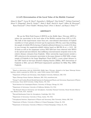
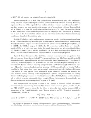
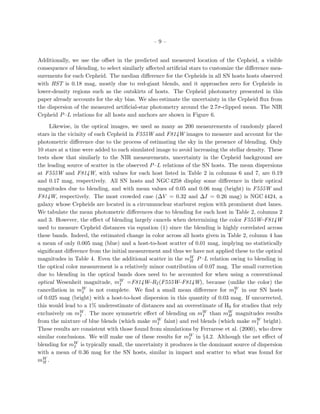
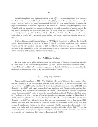
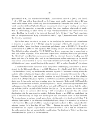
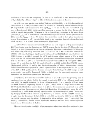
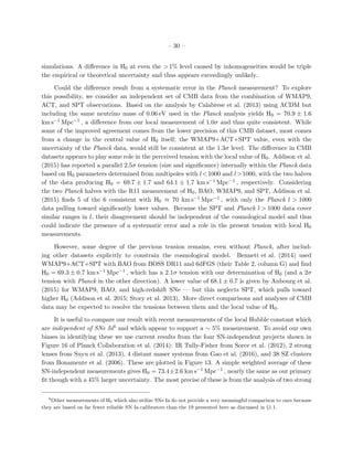
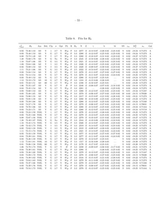
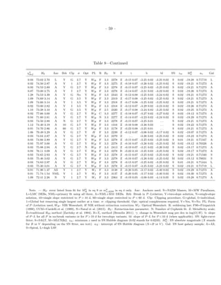
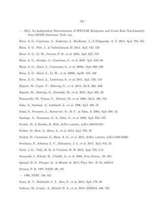
Table 2. Artificial Cepheid Tests in Optical Images
Host ∆V ∆I ∆ct ∆mW
I σ(V ) σ(I) σct σ(mW
I )
[mmag] [mag]
M101 6 3 1 -2 0.09 0.09 0.03 0.16
N1015 41 40 1 27 0.13 0.13 0.06 0.31
N1309 105 63 12 -1 0.35 0.26 0.10 0.48
N1365 15 19 0 7 0.13 0.13 0.06 0.29
N1448 31 24 1 6 0.14 0.13 0.06 0.29
N2442 141 109 8 23 0.24 0.21 0.10 0.48
N3021 106 134 0 75 0.23 0.22 0.09 0.46
N3370 69 55 5 26 0.23 0.19 0.07 0.37
N3447 34 23 4 -1 0.14 0.12 0.06 0.29
N3972 79 68 7 25 0.18 0.17 0.07 0.38
N3982 82 69 0 22 0.22 0.19 0.09 0.44
N4038 38 28 2 12 0.19 0.15 0.07 0.34
N4258I 5 7 -1 10 0.20 0.23 0.05 0.36
N4258O -2 1 0 0 0.08 0.07 0.02 0.10
N4424 318 262 -2 111 0.31 0.28 0.11 0.58
N4536 12 16 -1 10 0.11 0.10 0.05 0.24
N4639 56 85 -5 89 0.21 0.22 0.09 0.51
N5584 26 23 2 7 0.15 0.13 0.05 0.26
N5917 54 51 -2 32 0.20 0.19 0.08 0.42
N7250 152 91 13 -1 0.24 0.20 0.08 0.42
U9391 36 42 -3 38 0.15 0.15 0.06 0.34
Note. — ∆ = median magnitude or color offset derived from tests;
σ =dispersion around ∆; V stands for F555W; I stands for F814W;
ct= R × (V −I), with R = 0.39 for RV = 3.3 and the Fitzpatrick (1999)
extinction law; mW
I =defined in text.](https://image.slidesharecdn.com/a24determinationofthelocalvalueofthehubbleconstant-160604010334/85/A-2-4_determination_of_the_local_value_of_the_hubble_constant-10-320.jpg)
![– 13 –
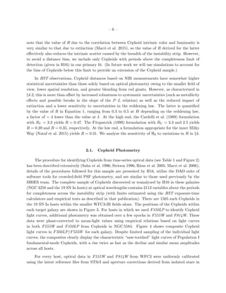
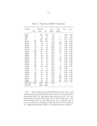
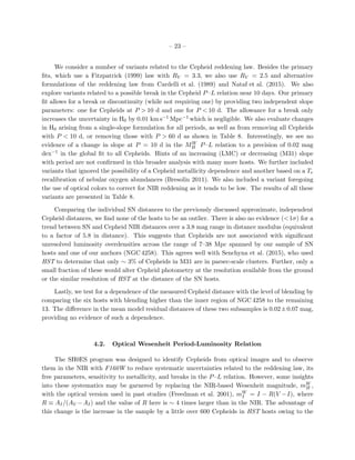
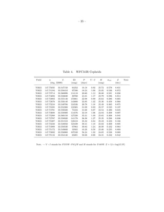
phase adds an error of σph =0.12 mag2. The relevant fractional contribution of the random-phase
uncertainty for a given Cepheid with period P depends on the temporal interval, ∆T, across NIR
epochs, a fraction we approximate as fph = 1 − (∆T/P) for ∆T <P and fph = 1 for ∆T >P; the
values of ∆T are given in Table 3. The value of this fraction ranges from ∼1 (NIR observations at
every optical epoch) to zero (a single NIR follow-up observation).
Thus, we assign a total statistical uncertainty arising from the quadrature sum of four terms:
NIR photometric error, color error, intrinsic width and random-phase:
σtot = (σ2
sky +σ2
ct+σ2
int+(fphσph)2
)
1
2 .
We give the values of σtot for each Cepheid in Table 4. These have a median of 0.30 mag (mean of
0.32 mag) across all fields; mean values for each field range from 0.23 mag (NGC 3447) to 0.47 mag
(NGC 4424). The mean for NGC 4258 is 0.39 mag. We also include in Table 4 an estimate of
the metallicity at the position of each Cepheid based on metallicity gradients measured from HII
regions and presented in H16.
3. Measuring the Hubble Constant
The determination of H0 follows the formalism described in §3 of R09. To summarize, we
perform a single, simultaneous fit to all Cepheid and SN Ia data to minimize one χ2 statistic and
measure the parameters of the distance ladder. We use the conventional definition of the distance
modulus, µ = 5 log D + 25, with D a luminosity distance in Mpc and measured as the difference in
magnitudes of an apparent and absolute flux, µ = m − M. We express the jth Cepheid magnitude
in the ith host as
mW
H,i,j = (µ0,i−µ0,N4258)+zpW,N4258+bW log Pi,j +ZW ∆ log [O/H]i,j, (2)
where the individual Cepheid parameters are given in Table 4 and mW
H,i,j was defined in Equation 1.
We determine the values of the nuisance parameters bW and ZW — which define the relation
between Cepheid period, metallicity, and luminosity — by minimizing the χ2 for the global fit to
the sample data. The reddening-free distances for the hosts relative to NGC 4258 are given by the
fit parameters µ0,i−µ0,N4258, while zpW,N4258 is the intercept of the P–L relation simultaneously fit
to the Cepheids of NGC 4258.
Uncertainties in the nuisance parameters are due to measurement errors and the limited period
and metallicity range spanned by the variables. In R11 we used a prior inferred from external
Cepheid datasets to help constrain these parameters. In the present analysis, instead, we explicitly
use external data as described below to augment the constraints.
2
The sum of the intrinsic and random phase errors, 0.14 mag, is smaller than the 0.21 mag assumed by R11; the
overestimate of this uncertainty explains why the χ2
of the P–L fits in that paper were low and resulted in the need
to rescale parameter errors.](https://image.slidesharecdn.com/a24determinationofthelocalvalueofthehubbleconstant-160604010334/85/A-2-4_determination_of_the_local_value_of_the_hubble_constant-13-320.jpg)
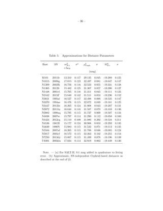
![– 15 –
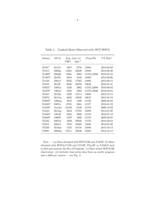
Observations of megamasers in Keplerian motion around a supermassive blackhole in NGC 4258
provide one of the best sources of calibration of the absolute distance scale with a total uncertainty
given by H13 of 3%. However, the leading systematic error in H13 resulted from limited numerical
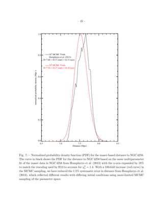
sampling of the multi-parameter model space of the system, given in H13 as 1.5%. The ongoing
improvement in computation speed allows us to reduce this error.
Here we make use of an improved distance estimate to NGC 4258 utilizing the same VLBI data
and model from H13 but now with a 100-fold increase in the number of Monte Carlo Markov Chain
(MCMC) trial values from 107 in that publication to 109 for each of three independent “strands” of
trials or initial guesses initialized near and at ±10% of the H13 distance. By increasing the number
of samples, the new simulation averages over many more of the oscillations of trial parameters in
an MCMC around their true values. The result is a reduction in the leading systematic error of
1.5% from H13 caused by “different initial conditions” for strands with only 107 MCMC samples
to 0.3% for the differences in strands with 109 MCMC samples. The smoother probability density
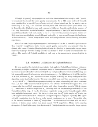
function (PDF) for the distance to NGC 4258 can be seen in Figure 7. The complete uncertainty
(statistical and systematic) for the maser distance to NGC 4258 is reduced from 3.0% to 2.6%, and
the better fit also produces a slight 0.8% decrease in the distance, yielding
D(NGC 4258) = 7.54 ± 0.17(random) ± 0.10(systematic) Mpc,
equivalent to µ0,N4258 = 29.387 ± 0.0568 mag.
The term ax in Equation 4 is the intercept of the SN Ia magnitude-redshift relation, approx-
imately log cz − 0.2m0
x in the low-redshift limit but given for an arbitrary expansion history and
for z >0 as
ax = log cz 1 +
1
2
[1 − q0] z −
1
6
1 − q0 − 3q2
0 + j0 z2
+ O(z3
) − 0.2m0
x, (5)
measured from the set of SN Ia (z, m0
x) independent of any absolute (i.e., luminosity or distance)
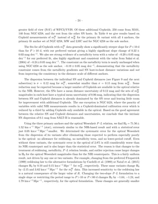
scale. We determine ax from a Hubble diagram of up to 281 SNe Ia with a light-curve fitter used to
find the individual m0
x as shown in Figure 8. Limiting the sample to 0.023<z <0.15 (to avoid the
possibility of a coherent flow in the more local volume; z is the redshift in the rest frame of the CMB
corrected for coherent flows, see §4.3) leaves 217 SNe Ia (in the next section we consider a lower cut
of z >0.01). Together with the present acceleration q0 = −0.55 and prior deceleration j0 = 1 which
can be measured via high-redshift SNe Ia (Riess et al. 2007; Betoule et al. 2014) independently of
the CMB or BAO, we find for the primary fit aB = 0.71273 ± 0.00176, with the uncertainty in q0
contributing 0.1% uncertainty (see §4.3). Combining the peak SN magnitudes to the intercept of
their Hubble diagram as m0
x,i + 5ax provides a measure of distance independent of the choice of
light-curve fitter, fiducial source, and measurement filter. These values are provided in Table 5.
We use matrix algebra to simultaneously express the over 1500 model equations in Equations 2
and 3, along with a diagonal correlation matrix containing the uncertainties. We invert the matrices
to derive the maximum-likelihood parameters, as in R09 and R11.](https://image.slidesharecdn.com/a24determinationofthelocalvalueofthehubbleconstant-160604010334/85/A-2-4_determination_of_the_local_value_of_the_hubble_constant-15-320.jpg)
![– 17 –
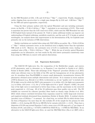
We add to this sample two more Cepheids with parallaxes measured by Riess et al. (2014)
and Casertano et al. (2015) using the WFC3 spatial scanning technique. These measurements have
similar fractional distance precision as those obtained with FGS despite their factor of 10 greater
distance and provide two of only four measured parallaxes for Cepheids with P >10 d. The resulting
parallax sample provides an independent anchor of our distance ladder with an error in their mean
of 1.6%, though this effectively increases to 2.2% after the addition of a conservatively estimated
σzp=0.03 mag zeropoint uncertainty between the ground and HST photometric systems (but see
discussion in §5).
We use the parallaxes and the H, V , and I-band photometry of the MW Cepheids by replacing
Equation 2 for the Cepheids in SN hosts and in M31 with
mW
H,i,j = µ0,i + MW
H,1 + bW log Pi,j + ZW ∆ log [O/H]i,j, (6)
where MW
H,1 is the absolute mW
H magnitude for a Cepheid with P = 1 d, and simultaneously fitting
the MW Cepheids with the relation
MW
H,i,j = MW
H,1+bW log Pi,j +ZW ∆ log [O/H]i,j, (7)
where MW
H,i,j = mW
H,i,j −µπ and µπ is the distance modulus derived from parallaxes, including
standard corrections for bias (often referred to as Lutz-Kelker bias) arising from the finite S/N
of parallax measurements with an assumed uncertainty of 0.01 mag (Hanson 1979). The H, V ,
and I-band photometry, measured from the ground, are transformed to match the WFC3 F160W,
F555W, and F814W as discussed in the next subsection. Equation 3 for the SNe Ia is replaced with
m0
x,i = µ0,i−M0
x. (8)
The determination of M0
x for SNe Ia together with the previous term ax then determines H0,
log H0 =
M0
x +5ax+25
5
. (9)
The statistical uncertainty in H0 is now derived from the quadrature sum of the two indepen-
dent terms in equation 9, M0
x and 5ax.
For mW
H Cepheid photometry not derived directly from HST WFC3, we assume a fully-
correlated uncertainty of 0.03 mag included as an additional, simultaneous constraint equation,
0 = ∆zp ± σzp, to the global constraints with σzp = 0.03 mag. The free parameter, ∆zp, which
expresses the zeropoint difference between HST WFC3 and ground-based data, is now added to
Equation 7 for all of the MW Cepheids. This is a convenience for tracking the correlation in
the zeropoints between ground-based data and providing an estimate of its size. In future work
we intend to eliminate ∆zp and its uncertainty by replacing the ground-based photometry with
measurements from HST WFC3 enabled by spatial scanning (Riess et al. 2014).](https://image.slidesharecdn.com/a24determinationofthelocalvalueofthehubbleconstant-160604010334/85/A-2-4_determination_of_the_local_value_of_the_hubble_constant-17-320.jpg)
![– 19 –
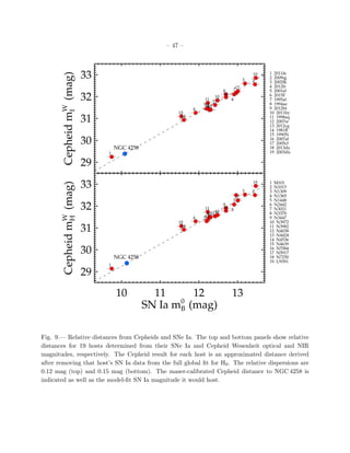
more modestly from 39 to 110. Similarly to the M31 Cepheids, the LMC Cepheids provide greater
precision for characterizing the P–L relations than those in the SN Ia hosts, and independently
hint at a change in slope at P ≈10 d (Bhardwaj et al. 2016).
We transform the ground-based V , I and H-band Vega-system photometry of Macri et al.
(2015) into the Vega-based HST/WFC3 photometric system in F555W, F814W and F160W, re-
spectively, using the following equations:
m555 = V + 0.034 + 0.11(V − I) (10)
m814 = I + 0.02 − 0.018(V − I) (11)
m160 = H + 0.16(J − H) (12)
where the color terms were derived from synthetic stellar photometry for the two systems using
SYNPHOT (Laidler et al. 2005). To determine any zeropoint offsets (aside from the potentially
different definitions of Vega) for the optical bands we compared photometry of 97 stars in the
LMC observed in V and I by OGLE-III and in WFC3/F555W and F814W as part of HST-GO
program #13010 (P.I.: Bresolin). The latter was calibrated following the exact same procedures
as H16, which uses the UVIS 2.0 WFC3 Vegamag zeropoints. The uncertainties of the zeropoints
in the optical transformations were found to be only 4 mmag. The change in color, V − I is quite
small, at 0.014 mag or a change (decrease) in H0 of 0.3 % for a value determined solely from
an anchor with ground-based Cepheid photometry (LMC or MW). For H-band transformed to
F160W, the net offset besides the aformentioned color term is zero after cancellation of an 0.02
mag offset measured between HST and 2MASS NIR photometry (Riess 2011) and the same in the
reverse direction from the very small count-rate non-linearity of WFC3 at the brightness level of
extragalactic Cepheids (Riess 2010). The mean metallicity of the LMC Cepheids is taken from
their spectra by Romaniello et al. (2008) to be [O/H] = −0.25 dex.
Using the late-type DEB distance to the LMC as the sole anchor and the Cepheid sample of
Macri et al. (2015) for a set of constraints in the form of Equation 7 yields H0 = 72.04 ± 2.56 km
s−1 Mpc−1 (stat). As in the prior section, these fits include free parameters ∆µLMC and ∆zp, with
additional constraint 0 = ∆µLMC ± σµ,LMC. The Appendix shows how the system of equations is
arranged for this fit. The last few equations (see Appendix) express the independent constraints on
the external distances (i.e., for NGC 4258 and the LMC) with uncertainties contained in the error
matrix.
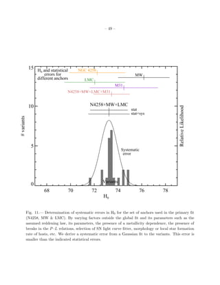
Using all three anchors, the same set used by R11 and by Efstathiou (2014), results in H0
= 73.24 ± 1.59 km s−1 Mpc−1(stat), a 2.2% determination. The fitted parameters which would
indicate consistency within the anchor sample are ∆µN4258 = −0.043 mag, within the range of
its 0.0568 mag prior, and ∆µLMC = −0.042 mag, within range of its 0.0452 mag prior. The
metallicity term for the NIR-based Wesenheit has the same sign but only about half the size as in
the optical (Sakai et al. 2004) and is not well-detected with ZW = −0.14±0.06 including systematic
uncertainties.](https://image.slidesharecdn.com/a24determinationofthelocalvalueofthehubbleconstant-160604010334/85/A-2-4_determination_of_the_local_value_of_the_hubble_constant-19-320.jpg)
![– 33 –
A. Setup of System of Equations
Equations 1 through 8 describe the relationships between the measurements and parameters
with additional constraint equations given in §3. To improve clarity we explicitly show the system
of equations we solve to derive the value of M0
B which together with the independent determi-
nation of aB provides the measurement of H0 via Equation 9. Here we refer to the vector of
measurements as y, the free parameters as q, the equation (or design) matrix as L, and the er-
ror matrix as C with χ2 = (y − Lq)T C−1(y − Lq) and maximum likelihood parameters given as
qbest = (LT C−1L)−1LT C−1y and covariance matrix (LT C−1L)−1. For the primary fit which uses 3
anchors, NGC 4258, Milky Way parallaxes, and LMC DEBs we arrange L, C and q as given below
so that some terms are fully correlated across a set of measurements like the anchor distances for
NGC 4258 and the LMC and ground-to-HST zeropoint errors are fully correlated and others like
the MW parallax distances are not.
y =
mW
H,1,j
..
mW
H,19,j
mW
H,j,N4258 − µ0,N4258
mW
H,M31,j
mW
H,MW,j − µπ,j
mW
H,LMC,j − µ0,LMC
m0
B,1
..
m0
B,19
0
0
0
l =
1 .. 0 0 1 0 0 log Ph
19,1/0 0 [O/H]19,1 0 log Pl
19,1/0
.. .. .. .. .. .. .. .. .. .. .. ..
0 .. 1 0 1 0 0 log Ph
19,j/0 0 [O/H]19,j 0 log Pl
19,j/0
0 .. 0 1 1 0 0 log Ph
N4258,j/0 0 [O/H]N4258,j 0 log Pl
N4258,j/0
0 .. 0 0 1 0 1 log Ph
M31,j/0 0 [O/H]M31,j 0 log Pl
M31,j/0
0 .. 0 0 1 0 0 log Ph
MW,j/0 0 [O/H]MW,j 1 log Pl
MW,j/0
0 .. 0 0 1 1 0 log Ph
LMC,j/0 0 [O/H]MW,j 1 log Pl
LMC,j/0
1 .. 0 0 0 0 0 0 1 0 0 0
0 .. 1 0 0 0 0 0 1 0 0 0
0 .. 0 0 0 0 0 0 0 0 1 0
0 .. 0 1 0 0 0 0 0 0 0 0
0 .. 0 0 0 1 0 0 0 0 0 0
](https://image.slidesharecdn.com/a24determinationofthelocalvalueofthehubbleconstant-160604010334/85/A-2-4_determination_of_the_local_value_of_the_hubble_constant-33-320.jpg)
![– 37 –
Table 6. Best Estimates of H0 Including Systematics
Anchor(s) Value
[km s−1
Mpc−1
]
One anchor
NGC 4258: Masers 72.25 ± 2.51
MW: 15 Cepheid Parallaxes 76.18 ± 2.37
LMC: 8 Late-type DEBs 72.04 ± 2.67
M31: 2 Early-type DEBs 74.50 ± 3.27
Two anchors
NGC 4258 + MW 74.04 ± 1.93
Three anchors (preferred)
NGC 4258 + MW + LMC 73.24 ± 1.74
Four anchors
NGC 4258 + MW + LMC + M31 73.46 ± 1.71
Optical only (no NIR), three anchors
NGC 4258 + MW + LMC 71.56 ± 2.49
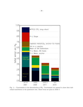
Table 7. H0 Error Budget for Cepheid and SN Ia Distance Ladders∗
Term Description Prev. R09 R11 This work
LMC N4258 All 3 N4258 All 3
σanchor Anchor distance, mean 5% 3% 1.3% 2.6% 1.3%
σa
anchorPL Mean of P–L in anchor 2.5% 1.5% 0.8% 1.2% 0.7%
σhostPL/
√
n Mean of P–L values in SN Ia hosts 1.5% 1.5% 0.6% 0.4% 0.4%
σSN/
√
n Mean of SN Ia calibrators 2.5% 2.5% 1.9% 1.2% 1.2%
σm−z SN Ia m–z relation 1% 0.5% 0.5% 0.4% 0.4%
Rσzp Cepheid reddening & colors, anchor-to-hosts 4.5% 0.3% 1.4% 0% 0.3%
σZ Cepheid metallicity, anchor-to-hosts 3% 1.1% 1.0% 0.0% 0.5%
σPL P–L slope, ∆ log P, anchor-to-hosts 4% 0.5% 0.6% 0.2% 0.5%
σWFPC2 WFPC2 CTE, long-short 3% N/A N/A N/A N/A
subtotal, σb
H0
10% 4.7% 2.9% 3.3%c
2.2%
Analysis Systematics N/A 1.3% 1.0% 1.2% 1.0%
Total, σH0
10% 4.8% 3.3% 3.5% 2.4%
Note. — (*) Derived from diagonal elements of the covariance matrix propagated via the error matrices
associated with Equations 1, 3, 7, and 8. (a) For MW parallax, this term is already included with the term
above. (b) For R09, R11, and this work, calculated with covariance included. (c) One anchor not included
in R11 estimate of σH0
to provide a crosscheck.](https://image.slidesharecdn.com/a24determinationofthelocalvalueofthehubbleconstant-160604010334/85/A-2-4_determination_of_the_local_value_of_the_hubble_constant-37-320.jpg)

![– 46 –
3.0
3.5
4.0
4.5
0.2mB(mag)
0.01 0.02 0.10 0.15 0.25 0.40z=
3.5 4.0 4.5 5.0
log (cz[1+0.5(1-q0)z-(1/6)(1-q0-3q0
2
+1)z2
])
-0.10
-0.05
0.00
0.05
0.10
∆0.2mB(mag)
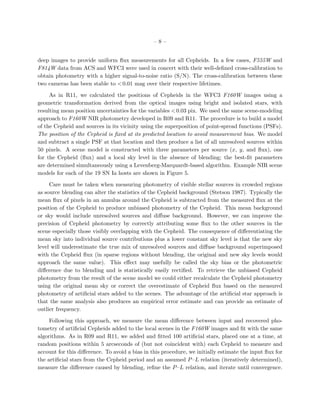
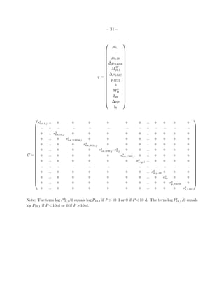
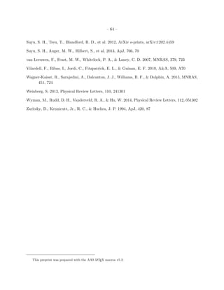
Fig. 8.— Hubble diagram of more than 600 SNe Ia at 0.01 < z < 0.4 in units of log cz. Mea-
surements of distance and redshift for a compilation of SN Ia data as described by Scolnic et al.
(2015). These data are used to determine the intercept, aX (see Equation 5) where log cz=0, which
helps measure the value of the Hubble constant as given in Equation 9). We account for changes
in the cosmological parameters empirically by including the kinematic terms, q0 and j0, measured
between high- and low-redshift SNe Ia. The intercept is measured using variants of this redshift
range, as discussed in the text, with the primary fit at 0.0233 < z < 0.15.](https://image.slidesharecdn.com/a24determinationofthelocalvalueofthehubbleconstant-160604010334/85/A-2-4_determination_of_the_local_value_of_the_hubble_constant-46-320.jpg)
![– 48 –
34
36
38
40
µ(z,H0=73.2,q0,j0)
Type Ia Supernovae → redshift(z)
29
30
31
32
33
SNIa:m-M(mag) Cepheids → Type Ia Supernovae
34 36 38 40
-0.4
0.0
0.4
∆mag
SN Ia: m-M (mag)
10
15
20
25
Geometry → Cepheids
Cepheid:m-M(mag)
Milky Way
LMC
M31
N4258
29 30 31 32 33
-0.4
0.0
0.4
∆mag
Cepheid: m-M (mag)
10 15 20 25
-0.4
-0.2
0.0
0.2
0.4
-0.4
0.0
0.4
∆mag
Geometry: 5 log D [Mpc] + 25
Fig. 10.— Complete distance ladder. The simultaneous agreement of pairs of geometric and
Cepheid-based distances (lower left), Cepheid and SN Ia-based distances (middle panel) and SN
and redshift-based distances provides the measurement of the Hubble constant. For each step,
geometric or calibrated distances on the x-axis serve to calibrate a relative distance indicator on
the y-axis through the determination of M or H0. Results shown are an approximation to the
global fit as discussed in the text.](https://image.slidesharecdn.com/a24determinationofthelocalvalueofthehubbleconstant-160604010334/85/A-2-4_determination_of_the_local_value_of_the_hubble_constant-48-320.jpg)
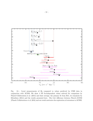

This document presents a 2.4% determination of the local value of the Hubble constant using new near-infrared observations of Cepheid variables in 11 host galaxies, improving on previous measurements. The study includes contributions from various geometric distance calibrations and reports a final estimate of H0 = 73.24 ± 1.74 km s−1 Mpc−1. It highlights discrepancies with predictions from the Lambda Cold Dark Matter model, suggesting potential implications for fundamental physics.


