Graph Analytics in machine learning programming

1. Graph Analytics
From managing and mining
graph data

2. What is the Diameter of this graph ?

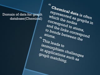
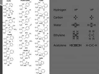
3. Domain of data for graph
database(Chemical)
 Chemical data is often
represented as graphs in
which the nodes
correspond to atoms,
and the links correspond
to bonds between the
atoms.
 This leads to
isomorphism challenges
in applications such as
graph matching.

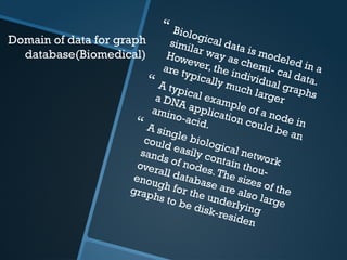
4. Domain of data for graph
database(Biomedical)
 Biological data is modeled in a
similar way as chemi- cal data.
However, the individual graphs
are typically much larger
 A typical example of a node in
a DNA application could be an
amino-acid.
 A single biological network
could easily contain thou-
sands of nodes.The sizes of the
overall database are also large
enough for the underlying
graphs to be disk-residen

6. Domain of data for
computer network
 In the case of computer net- works
and the web, the number of nodes in
the underlying graph may be massive.
 Since the number of nodes is massive,
this can lead to a very large number
of distinct edges.This is also referred
to as the massive domain issue in
networked data. In such cases, the
number of distinct edges may be so
large, that they may be hard to hold in
the available storage space.
 Thus, techniques need to be
designed to summarize and work with
condensed representations of the
graph data sets

7. Graph Query Language
 GraphLog (http://dl.acm.org/citation.cfm?id=298591)
 GOOD, which has its roots in object-oriented databases,
defines a transformation language that contains five basic
operations on graphs.
 GraphDB, another object-oriented data model and query
language for graphs, performs queries in four steps
 Unlike previous graph query lan- guages that operate on
nodes, edges, or paths, GraphQL [97] operates directly on
graphs.

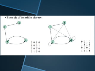
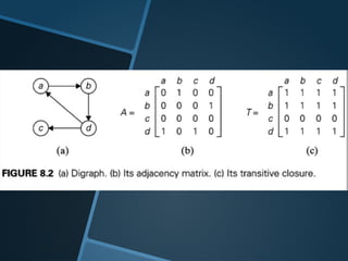
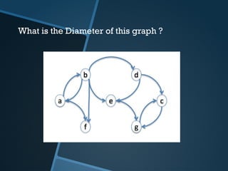
8. Reachability Queries
 Graph reachability queries test whether there is a path from a node to another
𝑣
node in a large directed graph.
𝑢
 Querying for reachability is a very basic operation that is important to many
applications, including applications in semantic web, biology networks, XML
query processing, etc
 Reachability queries can be answered by two obvious method :
 traverse the graph starting from node using breath- or depth-first search to see whether
𝑣
we can ever reach node .The query time is ( + )
𝑢 𝑂 𝑛 𝑚
 compute and store the edge transitive closure of the graph.With the transitive closure,
which requires ( 2) storage, a reachability query can be answered in (1) time by simply
𝑂 𝑛 𝑂
checking whether ( , ) is in the transitive closure.
𝑢 𝑣
 Research in this area focuses on finding the best compromise between the ( + )
𝑂 𝑛 𝑚
query time and the ( 2) storage cost.
𝑂 𝑛


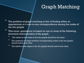
11. Graph Matching
 The problem of graph matching is that of finding either an
approximate or a one-to-one correspondence among the nodes of
the two graphs
 This corre- spondence is based on one or more of the following
structural characteristics of the graph:
 The labels on the nodes in the two graphs should be the same.
 The existence of edges between corresponding nodes in the two graphs
should match each other
 The labels on the edges in the two graphs should match each other.

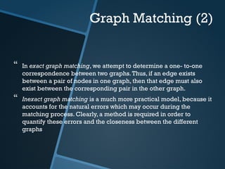
12. Graph Matching (2)
 In exact graph matching, we attempt to determine a one- to-one
correspondence between two graphs.Thus, if an edge exists
between a pair of nodes in one graph, then that edge must also
exist between the corresponding pair in the other graph.
 Inexact graph matching is a much more practical model, because it
accounts for the natural errors which may occur during the
matching process. Clearly, a method is required in order to
quantify these errors and the closeness between the different
graphs

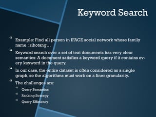
13. Keyword Search
 Example: Find all person in IFACE social network whose family
name : sihotang…
 Keyword search over a set of text documents has very clear
semantics: A document satisfies a keyword query if it contains ev-
ery keyword in the query.
 In our case, the entire dataset is often considered as a single
graph, so the algorithms must work on a finer granularity.
 The challenges are:
 Query Semantics
 Ranking Strategy
 Query Efficiency

14. Clustering Algorithms
Node Clustering Algorithm
Graph Clustering Algorithm

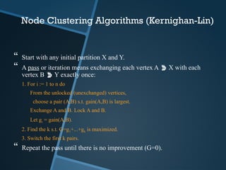
15. Node Clustering Algorithms (Kernighan-Lin)
 Start with any initial partition X and Y.
 A pass or iteration means exchanging each vertex A  X with each
vertex B  Y exactly once:
1. For i := 1 to n do
From the unlocked (unexchanged) vertices,
choose a pair (A,B) s.t. gain(A,B) is largest.
Exchange A and B. Lock A and B.
Let gi = gain(A,B).
2. Find the k s.t. G=g1+...+gk is maximized.
3. Switch the first k pairs.
 Repeat the pass until there is no improvement (G=0).

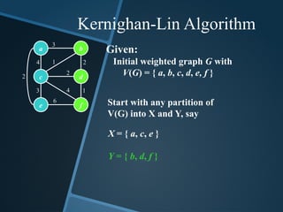
16. Kernighan-Lin Algorithm
Given:
Initial weighted graph G with
V(G) = { a, b, c, d, e, f }
a
c
b
d
e f
3
1
2
4
3 4
6
2
1
2
Start with any partition of
V(G) into X and Y, say
X = { a, c, e }
Y = { b, d, f }

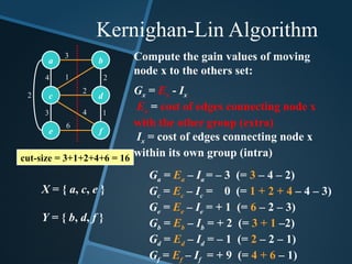
17. cut-size = 3+1+2+4+6 = 16
Ga = Ea – Ia = – 3 (= 3 – 4 – 2)
Gc = Ec – Ic = 0 (= 1 + 2 + 4 – 4 – 3)
Ge = Ee – Ie = + 1 (= 6 – 2 – 3)
Gb = Eb – Ib = + 2 (= 3 + 1 –2)
Gd = Ed – Id = – 1 (= 2 – 2 – 1)
Gf = Ef – If = + 9 (= 4 + 6 – 1)
Compute the gain values of moving
node x to the others set:
Gx = Ex - Ix
Ex = cost of edges connecting node x
with the other group (extra)
Ix = cost of edges connecting node x
within its own group (intra)
a
c
b
d
e f
3
1
2
4
3 4
6
2
1
2
X = { a, c, e }
Y = { b, d, f }
Kernighan-Lin Algorithm

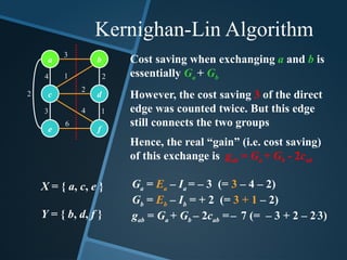
18. Ga = Ea – Ia = – 3 (= 3 – 4 – 2)
Gb = Eb – Ib = + 2 (= 3 + 1 – 2)
gab = Ga + Gb – 2cab =– 7 (= – 3 + 2 – 2.
3)
Cost saving when exchanging a and b is
essentially Ga + Gb
However, the cost saving 3 of the direct
edge was counted twice. But this edge
still connects the two groups
Hence, the real “gain” (i.e. cost saving)
of this exchange is gab = Ga + Gb - 2cab
a
c
b
d
e f
3
1
2
4
3 4
6
2
1
2
X = { a, c, e }
Y = { b, d, f }
Kernighan-Lin Algorithm

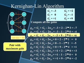
19. gab = Ga + Gb – 2wab = –3 + 2 – 23 = –7
gad = Ga + Gd – 2wad = –3 – 1 – 20 = –4
gaf = Ga + Gf – 2waf = –3 + 9 – 20 = +6
gcb = Gc + Gb – 2wcb = 0 + 2 – 21 = 0
gcd = Gc + Gd – 2wcd = 0 – 1 – 22 = –5
gcf = Gc + Gf – 2wcf = 0 + 9 – 24 = +1
geb = Ge + Gb – 2web = +1 + 2 – 20 = +3
ged = Ge + Gd – 2wed = +1 – 1 – 20 = 0
gef = Ge + Gf – 2wef = +1 + 9 – 26 = –2
Ga = –3 Gb = +2
Gc = 0 Gd = –1
Ge = +1 Gf = +9
Compute all the gains
a
c
b
d
e f
3
1
2
4
3 4
6
2
1
2
cut-size = 16
Pair with
maximum gain
Kernighan-Lin Algorithm

20. a
c
b
d
e
f
3
1
2
4
3 4
6
2
1
2
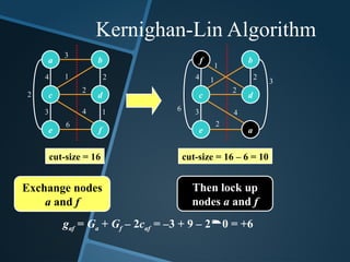
cut-size = 16 – 6 = 10
a
c
b
d
e f
3
1
2
4
3 4
6
2
1
2
cut-size = 16
Exchange nodes
a and f
gaf = Ga + Gf – 2caf = –3 + 9 – 20 = +6
Then lock up
nodes a and f
Kernighan-Lin Algorithm

21. a
c
b
d
e
f
3
1
2
4
3 4
6
2
1
2
cut-size = 10
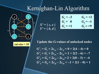
Update the G-values of unlocked nodes
Ga = –3 Gb = +2
Gc = 0 Gd = –1
Ge = +1 Gf = +9
G’c = Gc + 2cca – 2ccf = 0 + 2(4 – 4) = 0
G’e = Ge + 2cea – 2cef = 1 + 2(2 – 6) = –7
G’b = Gb + 2cbf – 2cba= 2 + 2(0 – 3) = –4
G’d = Gd + 2cdf – 2cda = –1 + 2(1 – 0) = 1
X’ = { c, e }
Y’ = { b, d }
Kernighan-Lin Algorithm

22. a
c
b
d
e
f
3
1
2
4
3 4
6
2
1
2
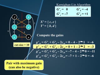
cut-size = 10
G’c = 0 G’b = –4
G’e = –7 G’d = +1
X’ = { c, e }
Y’ = { b, d }
Compute the gains
g’cb = G’c + G’b – 2ccb = 0 – 4 – 21 = –6
g’cd = G’c + G’d – 2ccd = 0 + 1 – 22 = –33
g’eb = G’e + G’b – 2ceb = –7 – 4 – 20 = –11
g’ed = G’e + G’d – 2ced = –7 + 1 – 20 = –6
Pair with maximum gain
(can also be negative)
Kernighan-Lin Algorithm

23. a
c
b
d
e
f
3
1
2
4
3 4
6
2
1
2
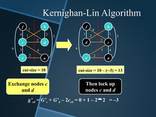
cut-size = 10
Exchange nodes c
and d
Then lock up
nodes c and d
a
d
b
c
e
f
3
1
2
4
3 4
6
2
1
2
cut-size = 10 – (–3) = 13
g’cd = G’c + G’d – 2ccd = 0 + 1 – 22 = –3
Kernighan-Lin Algorithm

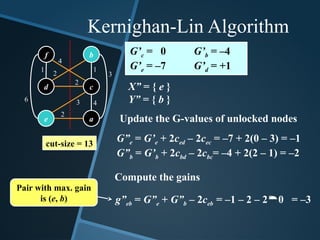
24. cut-size = 13
a
d
b
c
e
f
3
1
2
4
3 4
6
2
1
2
g”eb = G”e + G”b – 2ceb = –1 – 2 – 20 = –3
G’c = 0 G’b = –4
G’e = –7 G’d = +1
X” = { e }
Y” = { b }
Update the G-values of unlocked nodes
G”e = G’e + 2ced – 2cec = –7 + 2(0 – 3) = –1
G”b = G’b + 2cbd – 2cbc= –4 + 2(2 – 1) = –2
Compute the gains
Pair with max. gain
is (e, b)
Kernighan-Lin Algorithm

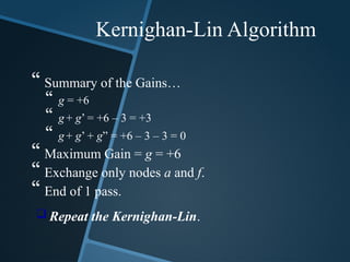
25.  Summary of the Gains…
 g = +6
 g+ g’ = +6 – 3 = +3
 g+ g’ + g” = +6 – 3 – 3 = 0
 Maximum Gain = g = +6
 Exchange only nodes a and f.
 End of 1 pass.
 Repeat the Kernighan-Lin.
Kernighan-Lin Algorithm

26. T
i
m
e
C
o
m
p
l
e
x
i
t
y
o
f
K
L
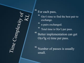
 For each pass,
 O(n2
) time to find the best pair to
exchange.
 n pairs exchanged.
 Total time is O(n3
) per pass.
 Better implementation can get
O(n2
lg n) time per pass.
 Number of passes is usually
small.

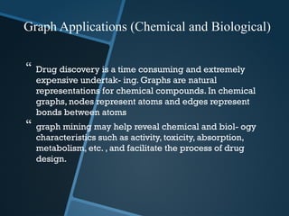
27.  Drug discovery is a time consuming and extremely
expensive undertak- ing. Graphs are natural
representations for chemical compounds. In chemical
graphs, nodes represent atoms and edges represent
bonds between atoms
 graph mining may help reveal chemical and biol- ogy
characteristics such as activity, toxicity, absorption,
metabolism, etc. , and facilitate the process of drug
design.
Graph Applications (Chemical and Biological)

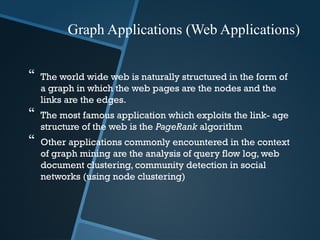
28.  The world wide web is naturally structured in the form of
a graph in which the web pages are the nodes and the
links are the edges.
 The most famous application which exploits the link- age
structure of the web is the PageRank algorithm
 Other applications commonly encountered in the context
of graph mining are the analysis of query flow log, web
document clustering, community detection in social
networks (using node clustering)
Graph Applications (Web Applications)

29.  Careful design of the underlying graph can
help avoid network failures, congestions, or
other weaknesses in the overall network.
 For example, centrality analysis can be used
in the context of a communication network
in order to determine criti- cal points of
failure
Graph Applications (Computer Network Applications)

30.  The goal of software bug localization techniques is to mine
such call graphs in order to determine the bugs in the
underlying programs
 static call graphs can be inferred from the source code of
a given program. All the methods, procedures and
functions in the program are nodes, and the relationships
between the different methods are defined as edges
 Dynamic call graphs are created during program
execution, and they represent the invocation structure. For
example, a call from one procedure to another creates an
edge which represents the invocation re- lationship
between the two procedures
Graph Applications (SW Bug Localization)