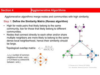
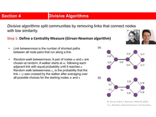
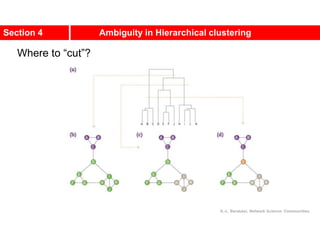
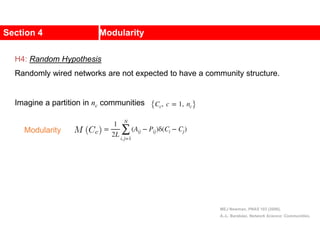
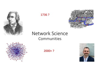
This document discusses Zachary's karate club network, which is a classic social network dataset. It contains three key points:
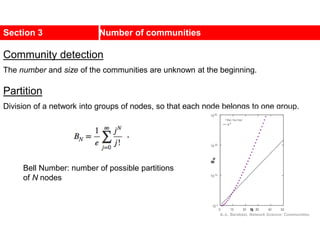
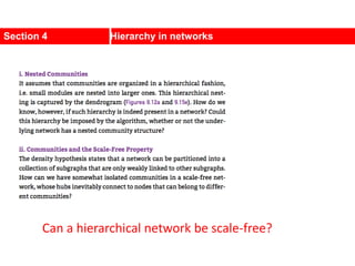
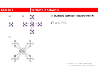
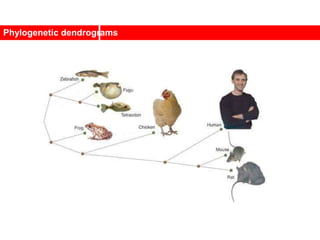
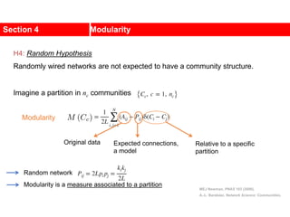
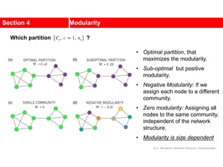
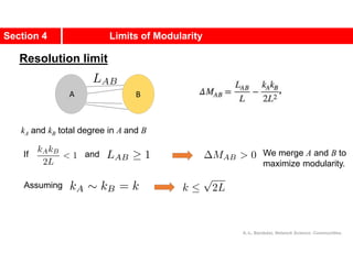
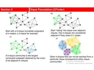
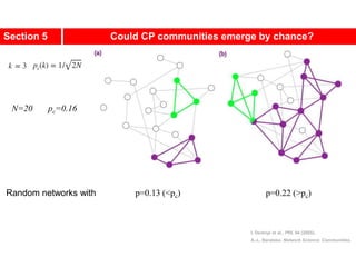
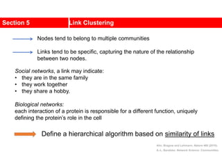
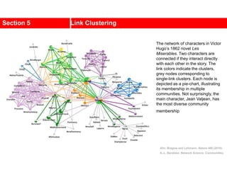
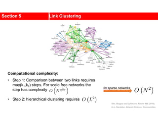
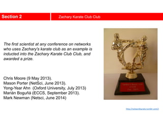
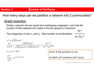
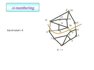
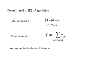
1. Zachary's karate club network describes the social ties between 34 members of a university karate club that split into two groups due to a conflict. This network is often used as an example for detecting community structure in networks.
2. The network was studied by Wayne Zachary from 1970-1972 and captured who interacted with whom both inside and outside the club. It correctly identified which group each member joined after the split except for one member.
3. The network became popular for studying community detection algorithms after being used in a 2002 paper by Michelle Girvan and Mark
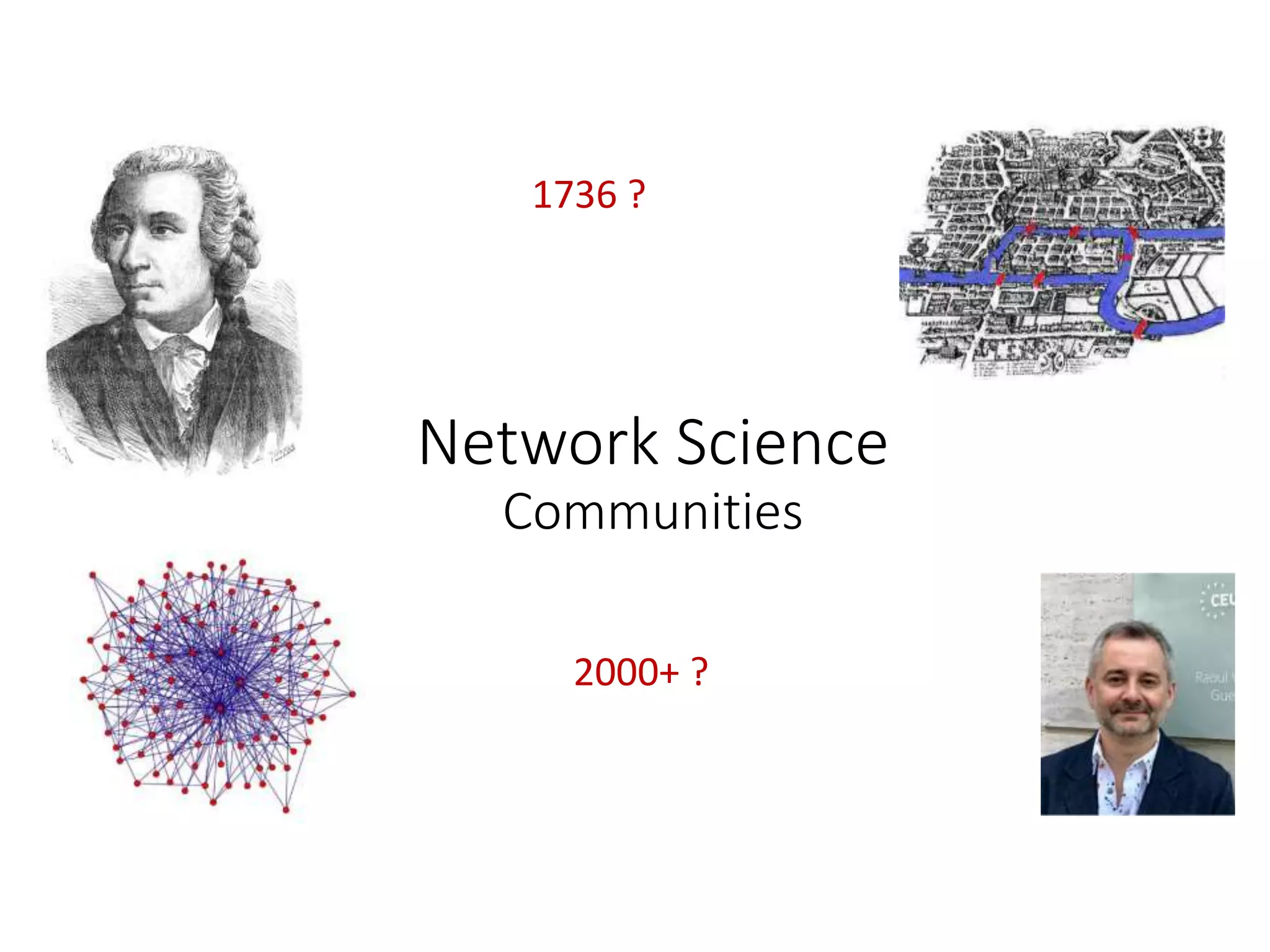
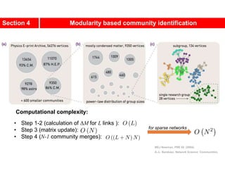
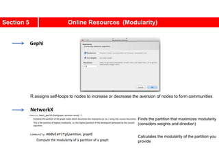
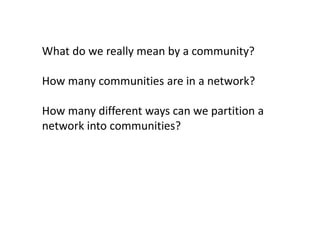
![A social network of a karate club was studied by Wayne
W. Zachary for a period of three years from 1970 to
1972.[2]
The network captures 34 members of a karate club,
documenting links between pairs of members who
interacted outside the club.
During the study a conflict arose between the
administrator "John A" and instructor "Mr. Hi"
(pseudonyms), which led to the split of the club into
two.
Half of the members formed a new club around Mr. Hi;
members from the other part found a new instructor or
gave up karate.
Based on collected data Zachary correctly assigned all
but one member of the club to the groups they actually
joined after the split.](https://image.slidesharecdn.com/ch-9communities-220816124612-4745b556/85/Communities-in-Network-Science-3-320.jpg)
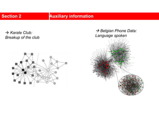

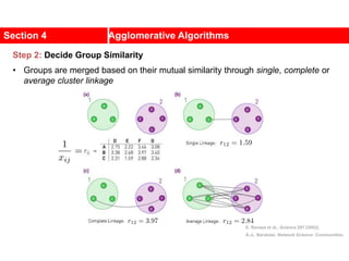
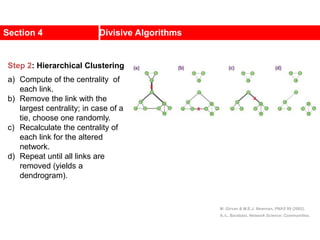
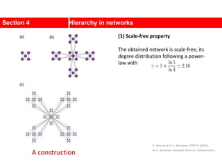
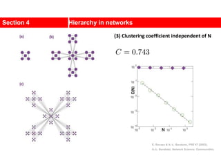
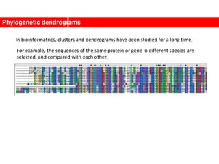
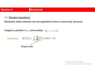
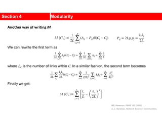
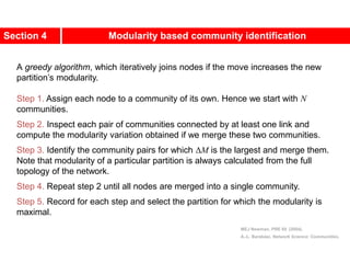
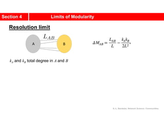
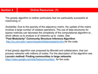
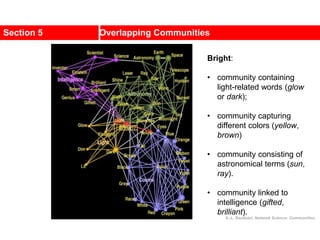
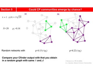
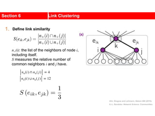
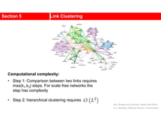
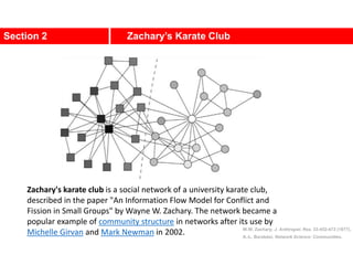
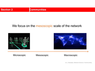
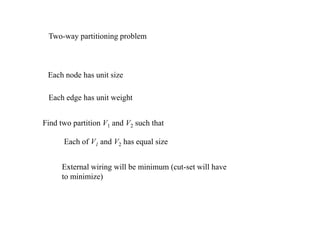
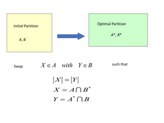
![Communities in Metabolic Networks
The E. coli metabolism offers a community structure of biological
systems [11].
a.The biological modules (communities) identified by the Ravasz
algorithm [11] (SECTION 9.3). The color of each node, capturing
the predominant biochemical class to which it belongs, indicates
that different functional classes are segregated in distinct
network neighborhoods. The highlighted region selects the nodes
that belong to the pyrimidine metabolism, one of the predicted
communities.
b.The topologic overlap matrix of the E. coli metabolism and the
corresponding dendrogram that allows us to identify the modules
shown in (a). The color of the branches reflect the predominant
biochemical role of the participating molecules, like
carbohydrates (blue), nucleotide and nucleic acid metabolism
(red), and lipid metabolism (cyan).
c.The red right branch of the dendrogram tree shown in (b),
highlighting the region corresponding to the pyridine module.
d.The detailed metabolic reactions within the pyrimidine module.
The boxes around the reactions highlight the communities
predicted by the Ravasz algorithm.](https://image.slidesharecdn.com/ch-9communities-220816124612-4745b556/85/Communities-in-Network-Science-9-320.jpg)
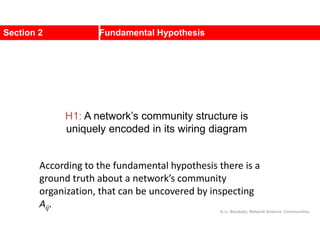


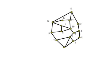
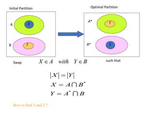
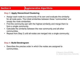
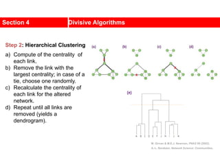
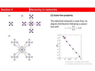
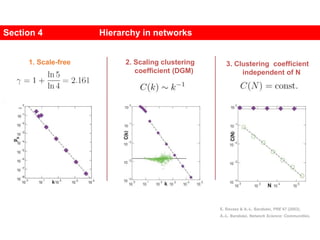
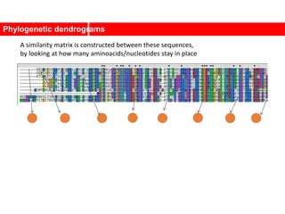
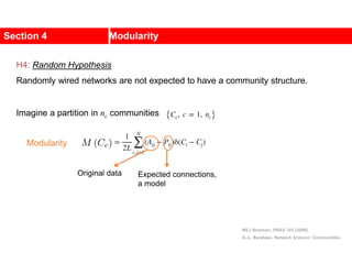
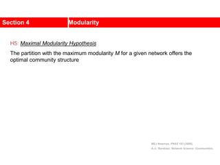
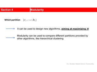
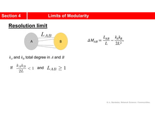
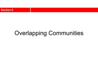
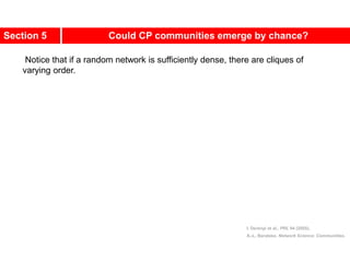
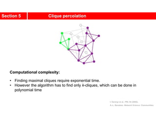
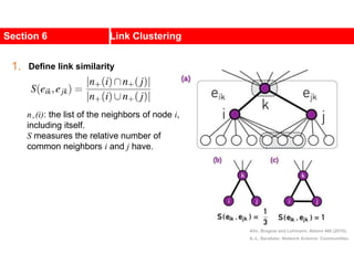
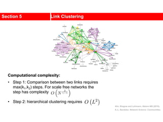
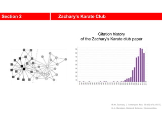
![Kernighan-Lin (KL) Example
a
b
c
d
e
f
g
h
4 { a, e } -2
0 -- 0
1 { d, g } 3
2 { c, f } 1
3 { b, h } -2
Step No. Vertex Pair Gain
5
5
2
1
3
Cut-cost
[©Sarrafzadeh]
Gain sum
0
3
4
2
0](https://image.slidesharecdn.com/ch-9communities-220816124612-4745b556/85/Communities-in-Network-Science-34-320.jpg)
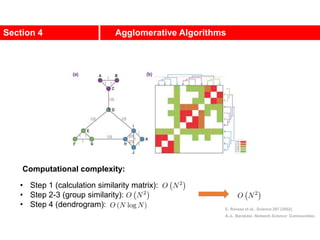
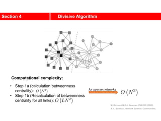
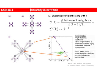
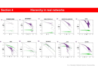
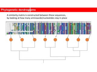
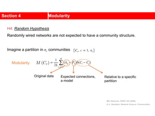
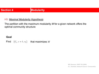
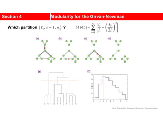
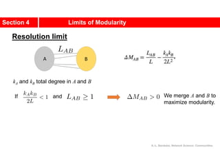
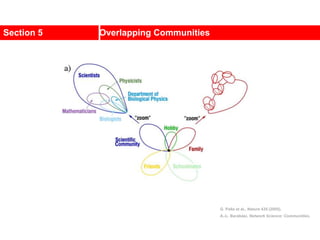
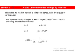
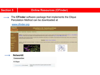
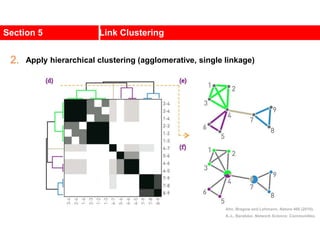
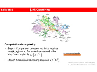
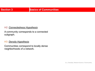
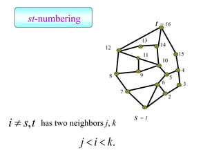
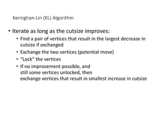
![Kernighan-Lin (KL) Example
a
b c
d
e
f
g
h
4 { a, e } -2
0 -- 0
1 { d, g } 3
2 { c, f } 1
3 { b, h } -2
Step No. Vertex Pair Gain
5
5
2
1
3
Cut-cost
[©Sarrafzadeh]
Gain sum
0
3
4
2
0](https://image.slidesharecdn.com/ch-9communities-220816124612-4745b556/85/Communities-in-Network-Science-35-320.jpg)
![Internal
cost
GA
GB
a1
a2
an
ai
a3
a5 a6
a4
b2
bj
b4 b3
b1
b6
b7
b5
A
x B
y
y
b
x
b
b
b
b
a
a
a
j
j
j
j
j
i
i
i
C
C
I
E
D
I
E
D
Likewise,
[©Kang]
External
cost
B
y
y
a
a
A
x
x
a
a i
i
i
i
C
E
C
I ,](https://image.slidesharecdn.com/ch-9communities-220816124612-4745b556/85/Communities-in-Network-Science-37-320.jpg)
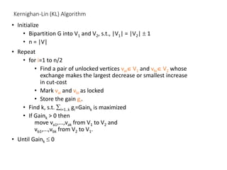
![• Lemma: Consider any ai A, bj B.
If ai, bj are interchanged, the gain is
• Proof:
Total cost before interchange (T) between A and B
Total cost after interchange (T’) between A and B
Therefore
Gain Calculation (cont.)
j
i
j
i b
a
b
a C
D
D
g 2
[©Kang]
others)
all
for
cost
(
j
i
j
i b
a
b
a C
E
E
T
others)
all
for
cost
(
j
i
j
i b
a
b
a C
I
I
T
j
i
j
j
i
i b
a
b
b
a
a C
I
E
I
E
T
T
g 2
i
a
D j
b
D](https://image.slidesharecdn.com/ch-9communities-220816124612-4745b556/85/Communities-in-Network-Science-38-320.jpg)
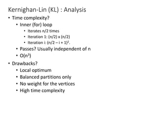
![Gain Calculation (cont.)
• Lemma:
• Let Dx’, Dy’ be the new D values for elements of
A - {ai} and B - {bj}. Then after interchanging ai & bj,
• Proof:
• The edge x-ai changed from internal in Dx to external in Dx’
• The edge y-bj changed from internal in Dx to external in Dx’
• The x-bj edge changed from external to internal
• The y-ai edge changed from external to internal
• More clarification in the next two slides
}
{
,
2
2
}
{
,
2
2
j
ya
yb
y
y
i
xb
xa
x
x
b
B
y
C
C
D
D
a
A
x
C
C
D
D
i
j
j
i
[©Kang]](https://image.slidesharecdn.com/ch-9communities-220816124612-4745b556/85/Communities-in-Network-Science-39-320.jpg)
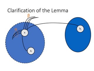
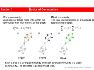
![Example: KL
• Step 1 - Initialization
A = {2, 3, 4}, B = {1, 5, 6}
A’ = A = {2, 3, 4}, B’ = B = {1, 5, 6}
• Step 2 - Compute D values
D1 = E1 - I1 = 1-0 = +1
D2 = E2 - I2 = 1-2 = -1
D3 = E3 - I3 = 0-1 = -1
D4 = E4 - I4 = 2-1 = +1
D5 = E5 - I5 = 1-1 = +0
D6 = E6 - I6 = 1-1 = +0
[©Kang]
5
6
4 2 1
3
Initial partition
4
5
6
2
3
1](https://image.slidesharecdn.com/ch-9communities-220816124612-4745b556/85/Communities-in-Network-Science-42-320.jpg)
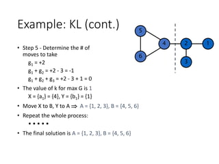
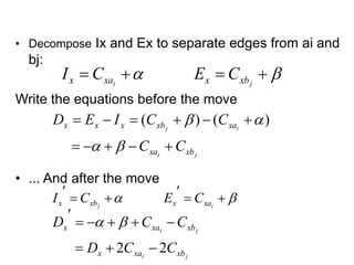
![Example: KL (cont.)
• Step 3 - compute gains
g21 = D2 + D1 - 2C21 = (-1) + (+1) - 2(1) = -2
g25 = D2 + D5 - 2C25 = (-1) + (+0) - 2(0) = -1
g26 = D2 + D6 - 2C26 = (-1) + (+0) - 2(0) = -1
g31 = D3 + D1 - 2C31 = (-1) + (+1) - 2(0) = 0
g35 = D3 + D5 - 2C35 = (-1) + (0) - 2(0) = -1
g36 = D3 + D6 - 2C36 = (-1) + (0) - 2(0) = -1
g41 = D4 + D1 - 2C41 = (+1) + (+1) - 2(0) = +2
g45 = D4 + D5 - 2C45 = (+1) + (+0) - 2(+1) = -1
g46 = D4 + D6 - 2C46 = (+1) + (+0) - 2(+1) = -1
• The largest g value is g41 = +2
interchange 4 and 1 (a1, b1) = (4, 1)
A’ = A’ - {4} = {2, 3}
B’ = B’ - {1} = {5, 6} both not empty
[©Kang]](https://image.slidesharecdn.com/ch-9communities-220816124612-4745b556/85/Communities-in-Network-Science-43-320.jpg)
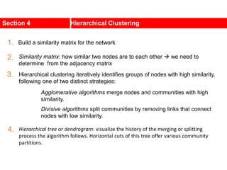
![Example: KL (cont.)
• Step 4 - update D values of node connected to vertices (4, 1)
D2’ = D2 + 2C24 - 2C21 = (-1) + 2(+1) - 2(+1) = -1
D5’ = D5 + 2C51 - 2C54 = +0 + 2(0) - 2(+1) = -2
D6’ = D6 + 2C61 - 2C64 = +0 + 2(0) - 2(+1) = -2
• Assign Di = Di’, repeat step 3 :
g25 = D2 + D5 - 2C25 = -1 - 2 - 2(0) = -3
g26 = D2 + D6 - 2C26 = -1 - 2 - 2(0) = -3
g35 = D3 + D5 - 2C35 = -1 - 2 - 2(0) = -3
g36 = D3 + D6 - 2C36 = -1 - 2 - 2(0) = -3
• All values are equal;
arbitrarily choose g36 = -3 (a2, b2) = (3, 6)
A’ = A’ - {3} = {2}, B’ = B’ - {6} = {5}
New D values are:
D2’ = D2 + 2C23 - 2C26 = -1 + 2(1) - 2(0) = +1
D5’ = D5 + 2C56 - 2C53 = -2 + 2(1) - 2(0) = +0
• New gain with D2 D2’, D5 D5’
g25 = D2 + D5 - 2C52 = +1 + 0 - 2(0) = +1 (a3, b3) = (2, 5) [©Kang]](https://image.slidesharecdn.com/ch-9communities-220816124612-4745b556/85/Communities-in-Network-Science-44-320.jpg)