7
Repeated Measures Designs
for Interval Data
Learning Objectives
After reading this chapter, you should be able to:
• Explain the advantages and drawbacks of using data from non-independent groups.
• Complete a paired-samples t-test.
• Complete a within-subjects F.
• Describe “power” as it relates to statistical testing.
iStockphoto/Thinkstock
tan81004_07_c07_163-192.indd 163 2/22/13 3:41 PM
CHAPTER 7Introduction
Chapter Outline
7.1 Dependent Groups Designs
Reconsidering the t and F ratios
An Example
A Matched Pairs Example
Comparing the Paired-Samples t-Test to the Independent Samples t-Test
The Power of the Dependent Groups Test
The Dependent Groups t-Test on Excel
The Alternate Approaches to Dependent t-Tests
7.2 The Within-Subjects F
Managing Error Variance in the Within-Subjects F
A Within-Subjects F Example
Calculating the Within-Subjects F
Understanding the Result
Comparing the Within-Subjects F and the One-Way ANOVA
Another Within-Subjects F Example
A Within-Subjects F in Excel
Chapter Summary
Introduction
Some of the most critical questions in management relate to change over time. For exam-ple, managers are deeply interested in assessing sales growth, shifts in shopping trends,
improvements in employee attitudes, increases in employee performance, and decreases in
absenteeism or turnover. They are also often keen to find out the influence of various
managerial decisions and business strategies on these and many other change-oriented
outcomes. However, none of the analyses completed to this point address these change-
related questions, because these analyses do not accommodate repeated measures of the
same variables within the same group of subjects over time. For instance, the t-tests and
ANOVAs discussed so far compared independent groups, groups that have completely
separate subjects. Each subject was only measured once on each variable of interest. The
same group of subjects was not measured repeatedly on the same variables to assess
change over time.
Another important issue is that independent samples t-tests and ANOVAs assume that
the groups being compared are equivalent on most aspects to begin with, except for the
independent (grouping or treatment) variable being investigated. When groups are large
and individuals are randomly selected, this is usually a reasonable assumption, because
any differences between groups tend to be relatively unimportant. The logic behind ran-
dom selection is that when groups are randomly drawn from the same population they
will differ only by chance—the larger the random sample, the lower the probability of
a substantial pre-existing difference. However, when groups are relatively small it can
be difficult to determine whether a difference in the measures of the dependent variable
occurred because the independent variable had a different impact on the different groups
or because there were differences between the groups to begin with.
tan81004_07.
Chapter 12Choosing an Appropriate Statistical TestiStockph.docxmccormicknadine86
Chapter 12
Choosing an Appropriate Statistical Test
iStockphoto/ThinkstockLearning Objectives
After reading this chapter, you will be able to. . .
· understand the importance of using the proper statistical analysis.
· identify the type of analysis based on four critical questions.
· use the decision tree to identify the correct statistical test.
Here we are in the final chapter that will pull all prior chapters together. Chapters 1 to 3 discussed descriptive statistics while the latterchapters, 4 to 11, discussed inferential statistics. Each of the inferential chapters presented a statistical concept then conducted the appropriateanalysis to be able to test a hypothesis. The big question for students learning statistics is, "How do I know if I'm using the correct statisticaltest?" For experienced statisticians this question is easy to answer as it is based on a few criteria. However, to a student just learning statisticsor to the novice researcher, this question is a legitimate one. Many statistical reference texts include a guide that asks specific questionsregarding the type of research question, design, number and scales of measurement of variables, and statistical assumption of the data thatallows you to use an elegant chart known as a decision tree. Based on the answers to these questions, the decision tree is used to helpdetermine the type of analysis to be used for the research, thereby helping you answer this big question.
12.1 Considerations
To make the correct decisions based on the use of a decision tree, there are four specific questions that must be answered. These questions areas follows:
· What is your overarching research question?
· How many independent, dependent, and covariate variables are used in the study?
· What are the scales of measurement of each of your variables?
· Are there violations of statistical assumptions?
If you are able to answer these specific questions, then you will be able to determine the proper analysis for your study. These questions arecritically important, and if they cannot be answered, then not enough thought has gone into the research. That said, let us discuss each ofthese questions so that they can be considered and answered in the use of the decision tree.
What Is Your Overarching Research Question?Try It!
Derive your ownresearch question foryour Master's Thesisor DoctoralDissertation. Have a colleague orprofessor read it. What are theirthoughts or suggestions forimprovements?
Answering this question seems simple enough as all research has an overarching research questionthat drives the study, especially since this dictates the type of quantitative methodology. There arekey words in every research question that help determine the appropriate type of analysis. Forinstance, if the research question states, "What are the effects of job satisfaction on employeeproductivity?" the keyword is "effects" as in the cause and effect of job satisfaction (theindependent variable) on productivity (th ...
Happiness Data SetAuthor Jackson, S.L. (2017) Statistics plain ShainaBoling829
Happiness Data Set
Author: Jackson, S.L. (2017) Statistics plain and simple. (4th ed.). Boston, MA: Cengage Learning.
I attach the previous essay so you have idea on how to do this assignment. It is similar to the assignment last week.
Assignment Content
1.
Top of Form
As you get closer to the final project in Week 6, you should have a better idea of the role of statistics in research. This week, you will calculate a one-way ANOVA for the independent groups. Reading and interpreting the output correctly is highly important. Most people who read research articles never see the actual output or data; they read the results statements by the researcher, which is why your summary must be accurate.
Consider your hypothesis statements you created in Part 2.
Calculate a one-way ANOVA, including a Tukey's HSD for the data from the Happiness and Engagement Dataset.
Write a 125- to 175-word summary of your interpretation of the results of the ANOVA, and describe how using an ANOVA was more advantageous than using multiple t tests to compare your independent variable on the outcome. Copy and paste your Microsoft® Excel® output below the summary.
Format your summary according to APA format.
Submit your summary, including the Microsoft® Excel® output to the assignment.
Reference/Module:
Module 13: Comparing More Than Two Groups
Using Designs with Three or More Levels of an Independent Variable
Comparing More than Two Kinds of Treatment in One Study
Comparing Two or More Kinds of Treatment with a Control Group
Comparing a Placebo Group to the Control and Experimental Groups
Analyzing the Multiple-Group Design
One-Way Between-Subjects ANOVA: What It Is and What It Does
Review of Key Terms
Module Exercises
Critical Thinking Check AnswersModule 14: One-Way Between-Subjects Analysis of Variance (ANOVA)
Calculations for the One-Way Between-Subjects ANOVA
Interpreting the One-Way Between-Subjects ANOVA
Graphing the Means and Effect Size
Assumptions of the One-Way Between-Subjects ANOVA
Tukey's Post Hoc Test
Review of Key Terms
Module Exercises
Critical Thinking Check AnswersChapter 7 Summary and ReviewChapter 7 Statistical Software Resources
In this chapter, we discuss the common types of statistical analyses used with designs involving more than two groups. The inferential statistics discussed in this chapter differ from those presented in the previous two chapters. In Chapter 5, single samples were being compared to populations (z test and t test), and in Chapter 6, two independent or correlated samples were being compared. In this chapter, the statistics are designed to test differences between more than two equivalent groups of subjects.
Several factors influence which statistic should be used to analyze the data collected. For example, the type of data collected and the number of groups being compared must be considered. Moreover, the statistic used to analyze the data will vary depending on whether the study involves a between-subjects design (designs in ...
5
ANOVA: Analyzing Differences
in Multiple Groups
Learning Objectives
After reading this chapter, you should be able to:
• Describe the similarities and differences between t-tests and ANOVA.
• Explain how ANOVA can help address some of the problems and limitations associ-
ated with t-tests.
• Use ANOVA to analyze multiple group differences.
• Use post hoc tests to pinpoint group differences.
• Determine the practical importance of statistically significant findings using effect
sizes with eta-squared.
iStockphoto/Thinkstock
tan81004_05_c05_103-134.indd 103 2/22/13 4:28 PM
CHAPTER 5Section 5.1 From t-Test to ANOVA
Chapter Overview
5.1 From t-Test to ANOVA
The ANOVA Advantage
Repeated Testing and Type I Error
5.2 One-Way ANOVA
Variance Between and Within
The Statistical Hypotheses
Measuring Data Variability in the ANOVA
Calculating Sums of Squares
Interpreting the Sums of Squares
The F Ratio
The ANOVA Table
Interpreting the F Ratio
Locating Significant Differences
Determining Practical Importance
5.3 Requirements for the One-Way ANOVA
Comparing ANOVA and the Independent t
One-Way ANOVA on Excel
5.4 Another One-Way ANOVA
Chapter Summary
Introduction
During the early part of the 20th century R. A. Fisher worked at an agricultural research station in rural southern England. In his work analyzing the effect of pesticides and
fertilizers on results like crop yield, he was stymied by the limitations in Gosset’s indepen-
dent samples t-test, which allowed him to compare just two samples at a time. In the effort
to develop a more comprehensive approach, Fisher created a statistical method he called
analysis of variance, often referred to by its acronym, ANOVA, which allows for making
multiple comparisons at the same time using relatively small samples.
5.1 From t-Test to ANOVA
The process for completing an independent samples t-test in Chapter 4 illustrated a number of things. The calculated t value, for example, is a score based on a ratio, one
determined by dividing the variability between the two groups (M1 2 M2) by the vari-
ability within the two groups, which is what the standard error of the difference (SEd)
measures. So both the numerator and the denominator of the t-ratio are measures of data
variability, albeit from different sources. The difference between the means is variability
attributed primarily to the independent variable, which is the group to which individual
subjects belong. The variability in the denominator is variability for reasons that are unex-
plained—error variance in the language of statistics.
tan81004_05_c05_103-134.indd 104 2/22/13 4:28 PM
CHAPTER 5Section 5.1 From t-Test to ANOVA
In his method, ANOVA, Fisher also embraced this
pattern of comparing between-groups variance to
within-groups variance. He calculated the variance
statistics differently, as we shall see, but he followed
Gosset’s pattern of a ratio of between-groups vari-
ance compared to within.
The ANOVA .
Technology-based assessments-special education
New technologies remain competitive in driving efforts to make learning more efficient. Technology-based assessment in special education has made quite some advancement (Goldsmith & LeBlanc, 2004). First applications of computer technology assessment were for the scoring student's test forms. Currently, features incorporate self-administration, software control in presentation, response evaluation based on algorithms, prescription based on expert knowledge and direct links in assessment and change in instructions. The technology-based assessment uses electronic and software systems to evaluate individual children in an educational setting. Traditional assessments employ approaches of the computer.
Video-based computer assisted test enabled learning of language for the student automatically increasing the validity of measurements. Video segments incorporated movie elements of moral dilemma in problem-solving tests. Students viewing the video segments respond by simply touching the screen. Innovative approaches have created relevance in testing procedures. Misplaced students result into poor results and get prompted to drop out. Teachers not well trained contribute to the misplacement due to poor management of certain behaviors and learning differences. For effect, teachers must be able to analyze data produced by the assessment and develop a due course of action.
In addressing students with physical limitations use of voice recognition, handwriting interpreters, stylus tools, and touchscreen enables communication without the use of keys (Gierach, 2009). New software features allow students to perform comfortable pace of video segments on preferred language options. Computers are linked to videodisc enabling students to learn according to individual needs and skills. Latest technological features concern evaluation. Technological advancements assess social competence among students. The evaluator views students in a variety of context. Limitation in technology infrastructure, seen as the key barrier in this sort of assessment. Many district schools lack adequate high-speed broadband access necessary for this evaluation. Moreover, obsolesce in technology-based assessment erodes the capacity to provide quality services technology-based systems have a relatively short functional life.
Holistic assessments are the best in technology-based assessments. They incorporate software control in presentation, conceptual models or algorithms, decision-making based rules and expert knowledge (Redecker, & Johannessen, 2013). Proliferation technology helps students in the inclusion of speech recognition, electronic communication, personal computers, robotics and artificial intelligence. Trends in technology-based assessments have impacted lives of students with a disability. They achieve school improvement goals as well as tracking student growth and progress. Current assessment norms have embedded current stan ...
3Type your name hereType your three-letter and -number cours.docxlorainedeserre
3
Type your name here
Type your three-letter and -number course code here
The date goes here
Type instructor’s name here
Your Title Goes Here
This is an electronic template for papers written in GCU style. The purpose of the template is to help you follow the basic writing expectations for beginning your coursework at GCU. Margins are set at 1 inch for top, bottom, left, and right. The first line of each paragraph is indented a half inch (0.5"). The line spacing is double throughout the paper, even on the reference page. One space after punctuation is used at the end of a sentence. The font style used in this template is Times New Roman. The font size is 12 point. When you are ready to write, and after having read these instructions completely, you can delete these directions and start typing. The formatting should stay the same. If you have any questions, please consult with your instructor.
Citations are used to reference material from another source. When paraphrasing material from another source (such as a book, journal, website), include the author’s last name and the publication year in parentheses.When directly quoting material word-for-word from another source, use quotation marks and include the page number after the author’s last name and year.
Using citations to give credit to others whose ideas or words you have used is an essential requirement to avoid issues of plagiarism. Just as you would never steal someone else’s car, you should not steal his or her words either. To avoid potential problems, always be sure to cite your sources. Cite by referring to the author’s last name, the year of publication in parentheses at the end of the sentence, such as (George & Mallery, 2016), and page numbers if you are using word-for-word materials. For example, “The developments of the World War II years firmly established the probability sample survey as a tool for describing population characteristics, beliefs, and attitudes” (Heeringa, West, & Berglund, 2017, p. 3).
The reference list should appear at the end of a paper (see the next page). It provides the information necessary for a reader to locate and retrieve any source you cite in the body of the paper. Each source you cite in the paper must appear in your reference list; likewise, each entry in the reference list must be cited in your text. A sample reference page is included below; this page includes examples (George & Mallery, 2016; Heeringa et al., 2017; Smith et al., 2018; “USA swimming,” 2018; Yu, Johnson, Deutsch, & Varga, 2018) of how to format different reference types (e.g., books, journal articles, and a website). For additional examples, see the GCU Style Guide.
References
George, D., & Mallery, P. (2016). IBM SPSS statistics 23 step by step: A simple guide and reference. New York, NY: Routledge.
Heeringa, S. G., West, B. T., & Berglund, P. A. (2017). Applied survey data analysis (2nd ed.). New York, NY: Chapman & Hall/CRC Press.
Smith, P. D., Martin, B., Chewning, B., ...
Between Black and White Population1. Comparing annual percent .docxjasoninnes20
Between Black and White Population
1. Comparing annual percent of Medicare enrollees having at least one ambulatory visit between B and W
2. Comparing average annual percent of diabetic Medicare enrollees age 65-75 having hemoglobin A1c between B and W
3. Comparing average annual percent of diabetic Medicare enrollees age 65-75 having eye examination between B and W
4. Comparing average annual percent of diabetic Medicare enrollees age 65-75 having
Students will develop an analysis report, in five main sections, including introduction, research method (research questions/objective, data set, research method, and analysis), results, conclusion and health policy recommendations. This is a 5-6 page individual project report.
Here are the main steps for this assignment.
Step 1: Students require to submit the topic using topic selection discussion forum by the end of week 1 and wait for instructor approval.
Step 2: Develop the research question and
Step 3: Run the analysis using EXCEL (RStudio for BONUS points) and report the findings using the assignment instruction.
The Report Structure:
Start with the
1.Cover page (1 page, including running head).
Please look at the example http://www.apastyle.org/manual/related/sample-experiment-paper-1.pdf (you can download the file from the class) and http://www.umuc.edu/library/libhow/apa_tutorial.cfm to learn more about the APA style.
In the title page include:
· Title, this is the approved topic by your instructor.
· Student name
· Class name
· Instructor name
· Date
2.Introduction
Introduce the problem or topic being investigated. Include relevant background information, for example;
· Indicates why this is an issue or topic worth researching;
· Highlight how others have researched this topic or issue (whether quantitatively or qualitatively), and
· Specify how others have operationalized this concept and measured these phenomena
Note: Introduction should not be more than one or two paragraphs.
Literature Review
There is no need for a literature review in this assignment
3.Research Question or Research Hypothesis
What is the Research Question or Research Hypothesis?
***Just in time information: Here are a few points for Research Question or Research Hypothesis
There are basically two kinds of research questions: testable and non-testable. Neither is better than the other, and both have a place in applied research.
Examples of non-testable questions are:
How do managers feel about the reorganization?
What do residents feel are the most important problems facing the community?
Respondents' answers to these questions could be summarized in descriptive tables and the results might be extremely valuable to administrators and planners. Business and social science researchers often ask non-testable research questions. The shortcoming with these types of questions is that they do not provide objective cut-off points for decision-makers.
In order to overcome this problem, researchers often seek to answer o ...
BUS 308 Week 3 Lecture 1 Examining Differences - Continued.docxcurwenmichaela
BUS 308 Week 3 Lecture 1
Examining Differences - Continued
Expected Outcomes
After reading this lecture, the student should be familiar with:
1. Issues around multiple testing
2. The basics of the Analysis of Variance test
3. Determining significant differences between group means
4. The basics of the Chi Square Distribution.
Overview
Last week, we found out ways to examine differences between a measure taken on two
groups (two-sample test situation) as well as comparing that measure to a standard (a one-sample
test situation). We looked at the F test which let us test for variance equality. We also looked at
the t-test which focused on testing for mean equality. We noted that the t-test had three distinct
versions, one for groups that had equal variances, one for groups that had unequal variances, and
one for data that was paired (two measures on the same subject, such as salary and midpoint for
each employee). We also looked at how the 2-sample unequal t-test could be used to use Excel
to perform a one-sample mean test against a standard or constant value. This week we expand
our tool kit to let us compare multiple groups for similar mean values.
A second tool will let us look at how data values are distributed – if graphed, would they
look the same? Different shapes or patterns often means the data sets differ in significant ways
that can help explain results.
Multiple Groups
As interesting as comparing two groups is, often it is a bit limiting as to what it tells us.
One obvious issue that we are missing in the comparisons made last week was equal work. This
idea is still somewhat hard to get a clear handle on. Typically, as we look at this issue, questions
arise about things such as performance appraisal ratings, education distribution, seniority impact,
etc.
Some of these can be tested with the tools introduced last week. We can see, for
example, if the performance rating average is the same for each gender. What we couldn’t do, at
this point however, is see if performance ratings differ by grade, do the more senior workers
perform relatively better? Is there a difference between ratings for each gender by grade level?
The same questions can be asked about seniority impact. This week will give us tools to expand
how we look at the clues hidden within the data set about equal pay for equal work.
ANOVA
So, let’s start taking a look at these questions. The first tool for this week is the Analysis
of Variance – ANOVA for short. ANOVA is often confusing for students; it says it analyzes
variance (which it does) but the purpose of an ANOVA test is to determine if the means of
different groups are the same! Now, so far, we have considered means and variance to be two
distinct characteristics of data sets; characteristics that are not related, yet here we are saying that
looking at one will give us insight into the other.
The reason is due to the way the variance is an.
BUS 308 Week 2 Lecture 2 Statistical Testing for Differenc.docxjasoninnes20
BUS 308 Week 2 Lecture 2
Statistical Testing for Differences – Part 1
After reading this lecture, the student should know:
1. How statistical distributions are used in hypothesis testing.
2. How to interpret the F test (both options) produced by Excel
3. How to interpret the T-test produced by Excel
Overview
Lecture 1 introduced the logic of statistical testing using the hypothesis testing procedure.
It also mentioned that we will be looking at two different tests this week. The t-test is used to
determine if means differ, from either a standard or claim or from another group. The F-test is
used to examine variance differences between groups.
This lecture starts by looking at statistical distributions – they underline the entire
statistical testing approach. They are kind of like the detective’s base belief that crimes are
committed for only a couple of reasons – money, vengeance, or love. The statistical distribution
that underlies each test assumes that statistical measures (such as the F value when comparing
variances and the t value when looking at means) follow a particular pattern, and this can be used
to make decisions.
While the underlying distributions differ for the different tests we will be looking at
throughout the course, they all have some basic similarities that allow us to examine the t
distribution and extrapolate from it to interpreting results based on other distributions.
Distributions. The basic logic for all statistical tests: If the null hypothesis claim is
correct, then the distribution of the statistical outcome will be distributed around a central value,
and larger and smaller values will be increasingly rare. At some point (and we define this as our
alpha value), we can say that the likelihood of getting a difference this large is extremely
unlikely and we will say that our results do not seem to come from a population that matches the
claims of the null hypothesis.
Note that this logic has several key elements:
1. The test is based on an assumption that the null hypothesis is correct. This gives us a
starting point, even if later proven wrong.
2. All sample results are turned into a statistic that matches the test selected (for
example, the F statistic when using the F-test, or the t-statistic when using the T-test.)
3. The calculated statistic is compared to a related statistical distribution to see how
likely an outcome we have.
4. The larger the test statistic, the more unlikely it is that the result matches or comes
from the population described by the null hypothesis claim.
We will demonstrate these ideas by looking at the questions being asked in this week’s
homework. We will show results of the related Excel tests, and discuss how to interpret the
output.
We need to remember that seeing different value (mean, variance, etc.) from different
samples does not tell us that the population parameters we are estimating are, in fact, different.
The ...
ANOVA is a hypothesis testing technique used to compare the equali.docxjustine1simpson78276
ANOVA is a hypothesis testing technique used to compare the equality of means for two or more groups; for example, it can be used to test that the mean number of computer chips produced by a company on each of the day, evening, and night shifts is the same. Give an example of an application of ANOVA in an industrial, operations, or manufacturing setting that is different from the examples provided in the overview. Discuss and share this information with your classmates.
In responding to your peers, select responses that use an ANOVA application that is different from your own. Are the results of the ANOVA application statistically significant? Why are the results significant or not significant? Explain your reasoning. Consider how ANOVA could be applied to the final project case study.
Support your initial posts and response posts with scholarly sources cited in APA style.
https://statistics4beginners.wordpress.com/2015/02/18/how-to-calculate-anova-in-excel-2013/
PLEASE GIVE A 1-2 PARAGRAPH RESPONSE TO THE FOLLOWING:
1.
In this module, our goal is to learn the statistical process of comparing several population means through a procedure called "analysis of variance", or ANOVA. ANOVA uses the variance from the mean of 2 or more sample populations to see if there is a statistically significant difference between them (Sharpe, DeVeaux, Velleman, 2016). We've learned that this is a valuable tool in all sorts of areas of study, including automotive, chemical, and medical industries.
There are many practical examples of ANOVA throughout business. As previously mentioned, the medical field can benefit from the use of this statistics tool. For example, a drug company may be interested in the results of clinical trials for a few new drugs they plan to release. Medicine A, B, and C are all now in the clinical testing phase, so the instances in which each cures a specific ailment can be summed up using ANOVA. Each of the individual drugs, through the course of multiple trials, will have a number of "cured" patients. The following is an example of what the results may be, in table format:
A B C
Trial 1 4 9 2
2 5 8 7
3 7 1 6
4 6 1 5
5 6 4 9
Using ANOVA to evaluate the variance from the mean for each trial, the ultimate goal would be to compare each trial to one another. By comparing the variance, we can say, with statistical confidence, that one medicine may be more effect.
MARKETING MANAGEMENT PHILOSOPHIES
CHAPTER 1 - ASSIGNMENT
Question 1.
Considering the differences of the philosophies, in some cases slight differences, select a company (product or service) and describe the current philosophy they pose for the customer. Include in your comments the level of customer value delivered by the company’s actions.
In other words, measure the company’s interaction with their customers against the Market Concept Philosophy. Does the company operate under the Market Concept Philosophy or do they lean more toward one of the other Philosophies.
Be specific with your examples.
DataSee comments at the right of the data set.IDSalaryCompaMidpointAgePerformance RatingServiceGenderRaiseDegreeGender1Grade8231.000233290915.80FAThe ongoing question that the weekly assignments will focus on is: Are males and females paid the same for equal work (under the Equal Pay Act)? 10220.956233080714.70FANote: to simplfy the analysis, we will assume that jobs within each grade comprise equal work.11231.00023411001914.80FA14241.04323329012160FAThe column labels in the table mean:15241.043233280814.90FAID – Employee sample number Salary – Salary in thousands 23231.000233665613.31FAAge – Age in yearsPerformance Rating – Appraisal rating (Employee evaluation score)26241.043232295216.21FAService – Years of service (rounded)Gender: 0 = male, 1 = female 31241.043232960413.90FAMidpoint – salary grade midpoint Raise – percent of last raise35241.043232390415.31FAGrade – job/pay gradeDegree (0= BS\BA 1 = MS)36231.000232775314.31FAGender1 (Male or Female)Compa - salary divided by midpoint37220.956232295216.21FA42241.0432332100815.70FA3341.096313075513.60FB18361.1613131801115.61FB20341.0963144701614.81FB39351.129312790615.51FB7411.0254032100815.70FC13421.0504030100214.71FC22571.187484865613.80FD24501.041483075913.81FD45551.145483695815.20FD17691.2105727553130FE48651.1405734901115.31FE28751.119674495914.41FF43771.1496742952015.51FF19241.043233285104.61MA25241.0432341704040MA40251.086232490206.30MA2270.870315280703.90MB32280.903312595405.60MB34280.903312680204.91MB16471.175404490405.70MC27401.000403580703.91MC41431.075402580504.30MC5470.9794836901605.71MD30491.0204845901804.30MD1581.017573485805.70ME4661.15757421001605.51ME12601.0525752952204.50ME33641.122573590905.51ME38560.9825745951104.50ME44601.0525745901605.21ME46651.1405739752003.91ME47621.087573795505.51ME49601.0525741952106.60ME50661.1575738801204.60ME6761.1346736701204.51MF9771.149674910010041MF21761.1346743951306.31MF29721.074675295505.40MF
Week 1Week 1.Measurement and Description - chapters 1 and 21Measurement issues. Data, even numerically coded variables, can be one of 4 levels - nominal, ordinal, interval, or ratio. It is important to identify which level a variable is, asthis impact the kind of analysis we can do with the data. For example, descriptive statistics such as means can only be done on interval or ratio level data.Please list under each label, the variabl ...
This is a lecture on "Hypothesis Testing, Research Questions and Choosing a Statistical Test". It was presented at the Colombo Institute for Research and Psychology. The lecture covers key topics including the different types of data, the process of testing a hypothesis, key forms of inferential statistical tests and how to chose a test based on your research question and sample.
Discussion Please discuss, elaborate and give example on the topiwiddowsonerica
Discussion: Please discuss, elaborate and give example on the topic below. Please use the Module/reference I provided. Professor will not allow outside sources.
Author: Jackson, S. L. (2017). Statistics plain and simple, (4th ed.). Boston, MA: Cengage Learning
Topic:
Using the sample provided, address the following:
· How would you interpret the results of the two-way ANOVA?
· What does the p value tell you?
· The results mention df. What does that term represent? How is it calculated? Write a plainly stated sentence that explains what these results tell you about the groups.
Sample
Sum of Squares df Mean Square F Sig.
SCORES Between Groups 351.520 4 87.880 9.085 .000
Within Groups 435.300 45 9.673
Total 7 86.820 49
Module/reference
Module 13: Comparing More Than Two Groups
Using Designs with Three or More Levels of an Independent Variable
Comparing More than Two Kinds of Treatment in One Study
Comparing Two or More Kinds of Treatment with a Control Group
Comparing a Placebo Group to the Control and Experimental Groups
Analyzing the Multiple-Group Design
One-Way Between-Subjects ANOVA: What It Is and What It Does
Review of Key Terms
Module Exercises
Critical Thinking Check Answers
Module 14: One-Way Between-Subjects Analysis of Variance (ANOVA)
Calculations for the One-Way Between-Subjects ANOVA
Interpreting the One-Way Between-Subjects ANOVA
Graphing the Means and Effect Size
Assumptions of the One-Way Between-Subjects ANOVA
Tukey's Post Hoc Test
Review of Key Terms
Module Exercises
Critical Thinking Check Answers
Chapter 7 Summary and Review
Chapter 7 Statistical Software Resources
In this chapter, we discuss the common types of statistical analyses used with designs involving more than two groups. The inferential statistics discussed in this chapter differ from those presented in the previous two chapters. In Chapter 5, single samples were being compared to populations (z test and t test), and in Chapter 6, two independent or correlated samples were being compared. In this chapter, the statistics are designed to test differences between more than two equivalent groups of subjects.
Several factors influence which statistic should be used to analyze the data collected. For example, the type of data collected and the number of groups being compared must be considered. Moreover, the statistic used to analyze the data will vary depending on whether the study involves a between-subjects design (designs in which different subjects are used in each group) or a correlated-groups design. (Remember, correlated-groups designs are of two types: within-subjects designs, in which the same subjects are used repeatedly in each group, and matched-subjects designs, in which different subjects are matched between conditions on variables that the researcher believes are relevant to the study.)
We will look at the typical inferential statistics used to analyze interval-ratio data for between-subjects designs. In Module 13 we discuss the advantages and rati ...
Discussion Please discuss, elaborate and give example on the topi.docxduketjoy27252
Discussion: Please discuss, elaborate and give example on the topic below. Please use the Module/reference I provided. Professor will not allow outside sources.
Author: Jackson, S. L. (2017). Statistics plain and simple, (4th ed.). Boston, MA: Cengage Learning
Topic:
Using the sample provided, address the following:
· How would you interpret the results of the two-way ANOVA?
· What does the p value tell you?
· The results mention df. What does that term represent? How is it calculated? Write a plainly stated sentence that explains what these results tell you about the groups.
Sample
Sum of Squares df Mean Square F Sig.
SCORES Between Groups 351.520 4 87.880 9.085 .000
Within Groups 435.300 45 9.673
Total 7 86.820 49
Module/reference
Module 13: Comparing More Than Two Groups
Using Designs with Three or More Levels of an Independent Variable
Comparing More than Two Kinds of Treatment in One Study
Comparing Two or More Kinds of Treatment with a Control Group
Comparing a Placebo Group to the Control and Experimental Groups
Analyzing the Multiple-Group Design
One-Way Between-Subjects ANOVA: What It Is and What It Does
Review of Key Terms
Module Exercises
Critical Thinking Check Answers
Module 14: One-Way Between-Subjects Analysis of Variance (ANOVA)
Calculations for the One-Way Between-Subjects ANOVA
Interpreting the One-Way Between-Subjects ANOVA
Graphing the Means and Effect Size
Assumptions of the One-Way Between-Subjects ANOVA
Tukey's Post Hoc Test
Review of Key Terms
Module Exercises
Critical Thinking Check Answers
Chapter 7 Summary and Review
Chapter 7 Statistical Software Resources
In this chapter, we discuss the common types of statistical analyses used with designs involving more than two groups. The inferential statistics discussed in this chapter differ from those presented in the previous two chapters. In Chapter 5, single samples were being compared to populations (z test and t test), and in Chapter 6, two independent or correlated samples were being compared. In this chapter, the statistics are designed to test differences between more than two equivalent groups of subjects.
Several factors influence which statistic should be used to analyze the data collected. For example, the type of data collected and the number of groups being compared must be considered. Moreover, the statistic used to analyze the data will vary depending on whether the study involves a between-subjects design (designs in which different subjects are used in each group) or a correlated-groups design. (Remember, correlated-groups designs are of two types: within-subjects designs, in which the same subjects are used repeatedly in each group, and matched-subjects designs, in which different subjects are matched between conditions on variables that the researcher believes are relevant to the study.)
We will look at the typical inferential statistics used to analyze interval-ratio data for between-subjects designs. In Module 13 we discuss the advantages and rati.
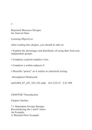
statistics/cf_choose_a_statistical_test (1) (1).pptx
Independent Variable [IV]
(number of groups)Dependent Variable [DV]
(measurement level) Two Groups
Three + Groups
Independent
(“unpaired”)Dependent
(“paired”)Independent
(“unpaired”)
Dependent
(“paired”)
CategoricalNon-parametric TestsChi-squareMcNemar’sChi-square
Cochran’s QOrdinal Mann-Whitney UWilcoxon Signed ranksKruskal Wallis HFriedman’sInterval / Ratio
(continuous)Parametric TestsIndependent
t-testDependent
t-testANOVARM-ANOVA
“What is the effect of TREATMENT (IV) on our OUTCOME (DV) of interest?”
Example: TREATMENT independent groups (placebo versus drug), OUTCOME interval/ratio (blood pressure)
Example: TREATMENT dependent group (pre/post yoga therapy), OUTCOME ordinal (back pain levels)
Example: TREATMENT independent 3+ groups (yoga therapy, none, aerobics), OUTCOME categorical (pass/fail of driving test)CorrelationsPhi coefficientSpearman’s rhoPearson’s r
Independent Variable
(number of groups)Dependent Variable (measurement level) Two Groups
Three + Groups
Independent
(“unpaired”)Dependent
(“paired”)Independent
(“unpaired”)
Dependent
(“paired”)
CategoricalNon-parametric TestsChi-squareMcNemar’sChi-square
Cochran’s QOrdinal Mann-Whitney UWilcoxon Signed ranksKruskal Wallis HFriedman’sInterval / Ratio
(continuous)Parametric TestsIndependent
t-testDependent
t-testANOVARM-ANOVA
STEP #1
Check what measurement level your DV is.
STEP #2
Choose the column related to the number Groups in your study.
STEP #3
Choose the column where intervention groups are either “paired” or “unpaired.”
STEP #4
Match your column with the row to find which test
to run.
STEP #1
Look at your Dependent Variable or outcome.
The data that we are looking at here is from the instruments you used to measure the effect of your intervention. Maybe you chose to measure stress with a commonly used psychological questionnaire or maybe you measured cholesterol levels or test scores.
What is its measurement level?
Categorical (such as yes or no; dead or alive; pass or fail).
Ordinal (such as health status – poor, average, excellent).
Interval ratio (for instance blood pressure, cholesterol level, rates of infection, or workplace satisfaction scores on a scale of 0-100).
STEP #2
Next you will look for the column that corresponds to the number of groups you have for your Independent Variable (also called experimental or predictor variable).
Remember, the independent variable is the thing in your study that was controlled by you (such as a medical intervention, or training initiative, or implementation of a modified protocol) for the purpose of making a change on some outcome in the population you are studying.
So…how many groups were involved in this intervention?
For example, if you were testing the effect of an evidence-based training initiative on employee workplace satisfaction or happiness, you might be interested in comparing the training initiative in one group to no training in another group..
WEEK 6 – EXERCISES Enter your answers in the spaces pr.docxwendolynhalbert
WEEK 6 – EXERCISES
Enter your answers in the spaces provided. Save the file using your last name as the beginning of the file name (e.g., ruf_week6_exercises) and submit via “Assignments.” When appropriate,
show your work
. You can do the work by hand, scan/take a digital picture, and attach that file with your work.
1
.
A psychotherapist studied whether his clients self-disclosed more while sitting in an easy chair or lying down on a couch. All clients had previously agreed to allow the sessions to be videotaped for research purposes. The therapist randomly assigned 10 clients to each condition. The third session for each client was videotaped and an independent observer counted the clients’ disclosures. The therapist reported that “clients made more disclosures when sitting in easy chairs (
M
= 18.20) than when lying down on a couch (
M
= 14.31),
t
(18) = 2.84,
p
< .05, two-tailed.” Explain these results to a person who understands the
t
test for a single sample but knows nothing about the
t
test for independent means.
2.
A researcher compared the adjustment of adolescents who had been raised in homes that were either very structured or unstructured. Thirty adolescents from each type of family completed an adjustment inventory. The results are reported in the table below. Explain these results to a person who understands the
t
test for a single sample but knows nothing about the
t
test for independent means.
Means on Four Adjustment Scales for
Adolescents from Structured versus Unstructured Homes
Scale
Structured Homes
Unstructured Homes
t
Social Maturity
106.82
113.94
–1.07
School Adjustment
116.31
107.22
2.03*
Identity Development
89.48
94.32
1.93*
Intimacy Development
102.25
104.33
.32
______________________
*
p
< .05
3.
Do men with higher levels of a particular hormone show higher levels of assertiveness? Levels of this hormone were tested in 100 men. The top 10 and the bottom 10 were selected for the study. All participants took part in a laboratory simulation in which they were asked to role-play a person picking his car up from a mechanic’s shop. The simulation was videotaped and later judged by independent raters on each of four types of assertive statements made by the participant. The results are shown in the table below. Explain these results to a person who fully understands the
t
test for a single sample but knows nothing about the
t
test for independent means.
Mean Number of Assertive Statements
Type of Assertive Statement
Group
1
2
3
4
Men with High Levels
2.14
1.16
3.83
0.14
Men with Low Levels
1.21
1.32
2.33
0.38
t
3.81**
0.89
2.03*
0.58
______________________
*
p
< .05;
**
p
< 0.1
4.
A manager of a small store wanted to discourage shoplifters by putting signs around the store saying “Shoplifting is a crime!” However, he wanted to make sure this would not result in customers buying less. To test this, he displayed the signs every other W.
For this Portfolio Project, you will write a paper about John A.docxevonnehoggarth79783
For this Portfolio Project, you will write a paper about "John Adams" as well as any event in U.S. history that is relevant to your major area of study or of interest to you. You will write about John Adams from the perspective of another historical personality who lived at the same time as the person or event you are going to describe.
For your historical personality, try to select someone from an under-represented population (examples of possible perspectives include that of Anne Hutchinson, Pocahontas, or Sojourner Truth). This analysis is to make you think about how events/people’s actions were interpreted at the time.
Key Points::
Remember that you will be writing from the perspective of a historical person about another person or an event from a period of U.S. history up to Reconstruction. From your historical person’s perspective, provide a thorough summary of the person or event you’ve chosen to write about, including the incidents that took place and any key individuals involved or affected.
Address the general importance of the person or event in the context of U.S. history.
Now, explain specifically how the person or event changed “your” daily life—“you” being the historical persona you have adopted.
Think long-term: How will the person or the event you are describing make a long-term impact in the lives of people who are in the under-represented group to which your historical person/perspective belongs?
Paper Requirements:
Your paper must be four to six pages, not including the required references and title pages.
Use at least five sources, not including the textbook. Include a scholarly journal article. Include at least one
primary
source from those identified in the syllabus.
Definition of a Primary Source
: A primary source is any source, document or artifact that was created at the time of the event. It was usually created by someone who witnessed the event, lived during or even shortly afterwards, or somehow would have first-hand knowledge of that event. A secondary source, by contrast, is written by a historian or someone writing about the event after it happened.
Have an introduction and strong thesis statement. Make use of support and examples supporting your thesis
Finish with a forceful conclusion reiterating your main idea.
Format your paper according to the
CSU-Global Guide to Writing and APA Requirements
(Links to an external site.)
.
.
For this portfolio assignment, you are required to research and anal.docxevonnehoggarth79783
For this portfolio assignment, you are required to research and analyze a TV program that ran between 1955 and 1965.
To successfully complete this essay, you will need to answer the following questions:
What is the background of this show? Explain what years it was on TV, describe the channel it aired on, the main characters, setting, etc..
What social issues and historical events were taking place at the time the show was being broadcast?
Did these issues affect the television show in any way?
Did the television show make an impact on popular culture?
Your thesis for the essay should attempt to answer this question:
Explain the cultural relevance of the show, given the information gathered from the show's background, and cultural history. How can television act as a reflection of the social, political, and cultural current events?
.
More Related Content
Similar to 7Repeated Measures Designs for Interval DataLearnin.docx
3Type your name hereType your three-letter and -number cours.docxlorainedeserre
3
Type your name here
Type your three-letter and -number course code here
The date goes here
Type instructor’s name here
Your Title Goes Here
This is an electronic template for papers written in GCU style. The purpose of the template is to help you follow the basic writing expectations for beginning your coursework at GCU. Margins are set at 1 inch for top, bottom, left, and right. The first line of each paragraph is indented a half inch (0.5"). The line spacing is double throughout the paper, even on the reference page. One space after punctuation is used at the end of a sentence. The font style used in this template is Times New Roman. The font size is 12 point. When you are ready to write, and after having read these instructions completely, you can delete these directions and start typing. The formatting should stay the same. If you have any questions, please consult with your instructor.
Citations are used to reference material from another source. When paraphrasing material from another source (such as a book, journal, website), include the author’s last name and the publication year in parentheses.When directly quoting material word-for-word from another source, use quotation marks and include the page number after the author’s last name and year.
Using citations to give credit to others whose ideas or words you have used is an essential requirement to avoid issues of plagiarism. Just as you would never steal someone else’s car, you should not steal his or her words either. To avoid potential problems, always be sure to cite your sources. Cite by referring to the author’s last name, the year of publication in parentheses at the end of the sentence, such as (George & Mallery, 2016), and page numbers if you are using word-for-word materials. For example, “The developments of the World War II years firmly established the probability sample survey as a tool for describing population characteristics, beliefs, and attitudes” (Heeringa, West, & Berglund, 2017, p. 3).
The reference list should appear at the end of a paper (see the next page). It provides the information necessary for a reader to locate and retrieve any source you cite in the body of the paper. Each source you cite in the paper must appear in your reference list; likewise, each entry in the reference list must be cited in your text. A sample reference page is included below; this page includes examples (George & Mallery, 2016; Heeringa et al., 2017; Smith et al., 2018; “USA swimming,” 2018; Yu, Johnson, Deutsch, & Varga, 2018) of how to format different reference types (e.g., books, journal articles, and a website). For additional examples, see the GCU Style Guide.
References
George, D., & Mallery, P. (2016). IBM SPSS statistics 23 step by step: A simple guide and reference. New York, NY: Routledge.
Heeringa, S. G., West, B. T., & Berglund, P. A. (2017). Applied survey data analysis (2nd ed.). New York, NY: Chapman & Hall/CRC Press.
Smith, P. D., Martin, B., Chewning, B., ...
Between Black and White Population1. Comparing annual percent .docxjasoninnes20
Between Black and White Population
1. Comparing annual percent of Medicare enrollees having at least one ambulatory visit between B and W
2. Comparing average annual percent of diabetic Medicare enrollees age 65-75 having hemoglobin A1c between B and W
3. Comparing average annual percent of diabetic Medicare enrollees age 65-75 having eye examination between B and W
4. Comparing average annual percent of diabetic Medicare enrollees age 65-75 having
Students will develop an analysis report, in five main sections, including introduction, research method (research questions/objective, data set, research method, and analysis), results, conclusion and health policy recommendations. This is a 5-6 page individual project report.
Here are the main steps for this assignment.
Step 1: Students require to submit the topic using topic selection discussion forum by the end of week 1 and wait for instructor approval.
Step 2: Develop the research question and
Step 3: Run the analysis using EXCEL (RStudio for BONUS points) and report the findings using the assignment instruction.
The Report Structure:
Start with the
1.Cover page (1 page, including running head).
Please look at the example http://www.apastyle.org/manual/related/sample-experiment-paper-1.pdf (you can download the file from the class) and http://www.umuc.edu/library/libhow/apa_tutorial.cfm to learn more about the APA style.
In the title page include:
· Title, this is the approved topic by your instructor.
· Student name
· Class name
· Instructor name
· Date
2.Introduction
Introduce the problem or topic being investigated. Include relevant background information, for example;
· Indicates why this is an issue or topic worth researching;
· Highlight how others have researched this topic or issue (whether quantitatively or qualitatively), and
· Specify how others have operationalized this concept and measured these phenomena
Note: Introduction should not be more than one or two paragraphs.
Literature Review
There is no need for a literature review in this assignment
3.Research Question or Research Hypothesis
What is the Research Question or Research Hypothesis?
***Just in time information: Here are a few points for Research Question or Research Hypothesis
There are basically two kinds of research questions: testable and non-testable. Neither is better than the other, and both have a place in applied research.
Examples of non-testable questions are:
How do managers feel about the reorganization?
What do residents feel are the most important problems facing the community?
Respondents' answers to these questions could be summarized in descriptive tables and the results might be extremely valuable to administrators and planners. Business and social science researchers often ask non-testable research questions. The shortcoming with these types of questions is that they do not provide objective cut-off points for decision-makers.
In order to overcome this problem, researchers often seek to answer o ...
BUS 308 Week 3 Lecture 1 Examining Differences - Continued.docxcurwenmichaela
BUS 308 Week 3 Lecture 1
Examining Differences - Continued
Expected Outcomes
After reading this lecture, the student should be familiar with:
1. Issues around multiple testing
2. The basics of the Analysis of Variance test
3. Determining significant differences between group means
4. The basics of the Chi Square Distribution.
Overview
Last week, we found out ways to examine differences between a measure taken on two
groups (two-sample test situation) as well as comparing that measure to a standard (a one-sample
test situation). We looked at the F test which let us test for variance equality. We also looked at
the t-test which focused on testing for mean equality. We noted that the t-test had three distinct
versions, one for groups that had equal variances, one for groups that had unequal variances, and
one for data that was paired (two measures on the same subject, such as salary and midpoint for
each employee). We also looked at how the 2-sample unequal t-test could be used to use Excel
to perform a one-sample mean test against a standard or constant value. This week we expand
our tool kit to let us compare multiple groups for similar mean values.
A second tool will let us look at how data values are distributed – if graphed, would they
look the same? Different shapes or patterns often means the data sets differ in significant ways
that can help explain results.
Multiple Groups
As interesting as comparing two groups is, often it is a bit limiting as to what it tells us.
One obvious issue that we are missing in the comparisons made last week was equal work. This
idea is still somewhat hard to get a clear handle on. Typically, as we look at this issue, questions
arise about things such as performance appraisal ratings, education distribution, seniority impact,
etc.
Some of these can be tested with the tools introduced last week. We can see, for
example, if the performance rating average is the same for each gender. What we couldn’t do, at
this point however, is see if performance ratings differ by grade, do the more senior workers
perform relatively better? Is there a difference between ratings for each gender by grade level?
The same questions can be asked about seniority impact. This week will give us tools to expand
how we look at the clues hidden within the data set about equal pay for equal work.
ANOVA
So, let’s start taking a look at these questions. The first tool for this week is the Analysis
of Variance – ANOVA for short. ANOVA is often confusing for students; it says it analyzes
variance (which it does) but the purpose of an ANOVA test is to determine if the means of
different groups are the same! Now, so far, we have considered means and variance to be two
distinct characteristics of data sets; characteristics that are not related, yet here we are saying that
looking at one will give us insight into the other.
The reason is due to the way the variance is an.
BUS 308 Week 2 Lecture 2 Statistical Testing for Differenc.docxjasoninnes20
BUS 308 Week 2 Lecture 2
Statistical Testing for Differences – Part 1
After reading this lecture, the student should know:
1. How statistical distributions are used in hypothesis testing.
2. How to interpret the F test (both options) produced by Excel
3. How to interpret the T-test produced by Excel
Overview
Lecture 1 introduced the logic of statistical testing using the hypothesis testing procedure.
It also mentioned that we will be looking at two different tests this week. The t-test is used to
determine if means differ, from either a standard or claim or from another group. The F-test is
used to examine variance differences between groups.
This lecture starts by looking at statistical distributions – they underline the entire
statistical testing approach. They are kind of like the detective’s base belief that crimes are
committed for only a couple of reasons – money, vengeance, or love. The statistical distribution
that underlies each test assumes that statistical measures (such as the F value when comparing
variances and the t value when looking at means) follow a particular pattern, and this can be used
to make decisions.
While the underlying distributions differ for the different tests we will be looking at
throughout the course, they all have some basic similarities that allow us to examine the t
distribution and extrapolate from it to interpreting results based on other distributions.
Distributions. The basic logic for all statistical tests: If the null hypothesis claim is
correct, then the distribution of the statistical outcome will be distributed around a central value,
and larger and smaller values will be increasingly rare. At some point (and we define this as our
alpha value), we can say that the likelihood of getting a difference this large is extremely
unlikely and we will say that our results do not seem to come from a population that matches the
claims of the null hypothesis.
Note that this logic has several key elements:
1. The test is based on an assumption that the null hypothesis is correct. This gives us a
starting point, even if later proven wrong.
2. All sample results are turned into a statistic that matches the test selected (for
example, the F statistic when using the F-test, or the t-statistic when using the T-test.)
3. The calculated statistic is compared to a related statistical distribution to see how
likely an outcome we have.
4. The larger the test statistic, the more unlikely it is that the result matches or comes
from the population described by the null hypothesis claim.
We will demonstrate these ideas by looking at the questions being asked in this week’s
homework. We will show results of the related Excel tests, and discuss how to interpret the
output.
We need to remember that seeing different value (mean, variance, etc.) from different
samples does not tell us that the population parameters we are estimating are, in fact, different.
The ...
ANOVA is a hypothesis testing technique used to compare the equali.docxjustine1simpson78276
ANOVA is a hypothesis testing technique used to compare the equality of means for two or more groups; for example, it can be used to test that the mean number of computer chips produced by a company on each of the day, evening, and night shifts is the same. Give an example of an application of ANOVA in an industrial, operations, or manufacturing setting that is different from the examples provided in the overview. Discuss and share this information with your classmates.
In responding to your peers, select responses that use an ANOVA application that is different from your own. Are the results of the ANOVA application statistically significant? Why are the results significant or not significant? Explain your reasoning. Consider how ANOVA could be applied to the final project case study.
Support your initial posts and response posts with scholarly sources cited in APA style.
https://statistics4beginners.wordpress.com/2015/02/18/how-to-calculate-anova-in-excel-2013/
PLEASE GIVE A 1-2 PARAGRAPH RESPONSE TO THE FOLLOWING:
1.
In this module, our goal is to learn the statistical process of comparing several population means through a procedure called "analysis of variance", or ANOVA. ANOVA uses the variance from the mean of 2 or more sample populations to see if there is a statistically significant difference between them (Sharpe, DeVeaux, Velleman, 2016). We've learned that this is a valuable tool in all sorts of areas of study, including automotive, chemical, and medical industries.
There are many practical examples of ANOVA throughout business. As previously mentioned, the medical field can benefit from the use of this statistics tool. For example, a drug company may be interested in the results of clinical trials for a few new drugs they plan to release. Medicine A, B, and C are all now in the clinical testing phase, so the instances in which each cures a specific ailment can be summed up using ANOVA. Each of the individual drugs, through the course of multiple trials, will have a number of "cured" patients. The following is an example of what the results may be, in table format:
A B C
Trial 1 4 9 2
2 5 8 7
3 7 1 6
4 6 1 5
5 6 4 9
Using ANOVA to evaluate the variance from the mean for each trial, the ultimate goal would be to compare each trial to one another. By comparing the variance, we can say, with statistical confidence, that one medicine may be more effect.
MARKETING MANAGEMENT PHILOSOPHIES
CHAPTER 1 - ASSIGNMENT
Question 1.
Considering the differences of the philosophies, in some cases slight differences, select a company (product or service) and describe the current philosophy they pose for the customer. Include in your comments the level of customer value delivered by the company’s actions.
In other words, measure the company’s interaction with their customers against the Market Concept Philosophy. Does the company operate under the Market Concept Philosophy or do they lean more toward one of the other Philosophies.
Be specific with your examples.
DataSee comments at the right of the data set.IDSalaryCompaMidpointAgePerformance RatingServiceGenderRaiseDegreeGender1Grade8231.000233290915.80FAThe ongoing question that the weekly assignments will focus on is: Are males and females paid the same for equal work (under the Equal Pay Act)? 10220.956233080714.70FANote: to simplfy the analysis, we will assume that jobs within each grade comprise equal work.11231.00023411001914.80FA14241.04323329012160FAThe column labels in the table mean:15241.043233280814.90FAID – Employee sample number Salary – Salary in thousands 23231.000233665613.31FAAge – Age in yearsPerformance Rating – Appraisal rating (Employee evaluation score)26241.043232295216.21FAService – Years of service (rounded)Gender: 0 = male, 1 = female 31241.043232960413.90FAMidpoint – salary grade midpoint Raise – percent of last raise35241.043232390415.31FAGrade – job/pay gradeDegree (0= BS\BA 1 = MS)36231.000232775314.31FAGender1 (Male or Female)Compa - salary divided by midpoint37220.956232295216.21FA42241.0432332100815.70FA3341.096313075513.60FB18361.1613131801115.61FB20341.0963144701614.81FB39351.129312790615.51FB7411.0254032100815.70FC13421.0504030100214.71FC22571.187484865613.80FD24501.041483075913.81FD45551.145483695815.20FD17691.2105727553130FE48651.1405734901115.31FE28751.119674495914.41FF43771.1496742952015.51FF19241.043233285104.61MA25241.0432341704040MA40251.086232490206.30MA2270.870315280703.90MB32280.903312595405.60MB34280.903312680204.91MB16471.175404490405.70MC27401.000403580703.91MC41431.075402580504.30MC5470.9794836901605.71MD30491.0204845901804.30MD1581.017573485805.70ME4661.15757421001605.51ME12601.0525752952204.50ME33641.122573590905.51ME38560.9825745951104.50ME44601.0525745901605.21ME46651.1405739752003.91ME47621.087573795505.51ME49601.0525741952106.60ME50661.1575738801204.60ME6761.1346736701204.51MF9771.149674910010041MF21761.1346743951306.31MF29721.074675295505.40MF
Week 1Week 1.Measurement and Description - chapters 1 and 21Measurement issues. Data, even numerically coded variables, can be one of 4 levels - nominal, ordinal, interval, or ratio. It is important to identify which level a variable is, asthis impact the kind of analysis we can do with the data. For example, descriptive statistics such as means can only be done on interval or ratio level data.Please list under each label, the variabl ...
This is a lecture on "Hypothesis Testing, Research Questions and Choosing a Statistical Test". It was presented at the Colombo Institute for Research and Psychology. The lecture covers key topics including the different types of data, the process of testing a hypothesis, key forms of inferential statistical tests and how to chose a test based on your research question and sample.
Discussion Please discuss, elaborate and give example on the topiwiddowsonerica
Discussion: Please discuss, elaborate and give example on the topic below. Please use the Module/reference I provided. Professor will not allow outside sources.
Author: Jackson, S. L. (2017). Statistics plain and simple, (4th ed.). Boston, MA: Cengage Learning
Topic:
Using the sample provided, address the following:
· How would you interpret the results of the two-way ANOVA?
· What does the p value tell you?
· The results mention df. What does that term represent? How is it calculated? Write a plainly stated sentence that explains what these results tell you about the groups.
Sample
Sum of Squares df Mean Square F Sig.
SCORES Between Groups 351.520 4 87.880 9.085 .000
Within Groups 435.300 45 9.673
Total 7 86.820 49
Module/reference
Module 13: Comparing More Than Two Groups
Using Designs with Three or More Levels of an Independent Variable
Comparing More than Two Kinds of Treatment in One Study
Comparing Two or More Kinds of Treatment with a Control Group
Comparing a Placebo Group to the Control and Experimental Groups
Analyzing the Multiple-Group Design
One-Way Between-Subjects ANOVA: What It Is and What It Does
Review of Key Terms
Module Exercises
Critical Thinking Check Answers
Module 14: One-Way Between-Subjects Analysis of Variance (ANOVA)
Calculations for the One-Way Between-Subjects ANOVA
Interpreting the One-Way Between-Subjects ANOVA
Graphing the Means and Effect Size
Assumptions of the One-Way Between-Subjects ANOVA
Tukey's Post Hoc Test
Review of Key Terms
Module Exercises
Critical Thinking Check Answers
Chapter 7 Summary and Review
Chapter 7 Statistical Software Resources
In this chapter, we discuss the common types of statistical analyses used with designs involving more than two groups. The inferential statistics discussed in this chapter differ from those presented in the previous two chapters. In Chapter 5, single samples were being compared to populations (z test and t test), and in Chapter 6, two independent or correlated samples were being compared. In this chapter, the statistics are designed to test differences between more than two equivalent groups of subjects.
Several factors influence which statistic should be used to analyze the data collected. For example, the type of data collected and the number of groups being compared must be considered. Moreover, the statistic used to analyze the data will vary depending on whether the study involves a between-subjects design (designs in which different subjects are used in each group) or a correlated-groups design. (Remember, correlated-groups designs are of two types: within-subjects designs, in which the same subjects are used repeatedly in each group, and matched-subjects designs, in which different subjects are matched between conditions on variables that the researcher believes are relevant to the study.)
We will look at the typical inferential statistics used to analyze interval-ratio data for between-subjects designs. In Module 13 we discuss the advantages and rati ...
Discussion Please discuss, elaborate and give example on the topi.docxduketjoy27252
Discussion: Please discuss, elaborate and give example on the topic below. Please use the Module/reference I provided. Professor will not allow outside sources.
Author: Jackson, S. L. (2017). Statistics plain and simple, (4th ed.). Boston, MA: Cengage Learning
Topic:
Using the sample provided, address the following:
· How would you interpret the results of the two-way ANOVA?
· What does the p value tell you?
· The results mention df. What does that term represent? How is it calculated? Write a plainly stated sentence that explains what these results tell you about the groups.
Sample
Sum of Squares df Mean Square F Sig.
SCORES Between Groups 351.520 4 87.880 9.085 .000
Within Groups 435.300 45 9.673
Total 7 86.820 49
Module/reference
Module 13: Comparing More Than Two Groups
Using Designs with Three or More Levels of an Independent Variable
Comparing More than Two Kinds of Treatment in One Study
Comparing Two or More Kinds of Treatment with a Control Group
Comparing a Placebo Group to the Control and Experimental Groups
Analyzing the Multiple-Group Design
One-Way Between-Subjects ANOVA: What It Is and What It Does
Review of Key Terms
Module Exercises
Critical Thinking Check Answers
Module 14: One-Way Between-Subjects Analysis of Variance (ANOVA)
Calculations for the One-Way Between-Subjects ANOVA
Interpreting the One-Way Between-Subjects ANOVA
Graphing the Means and Effect Size
Assumptions of the One-Way Between-Subjects ANOVA
Tukey's Post Hoc Test
Review of Key Terms
Module Exercises
Critical Thinking Check Answers
Chapter 7 Summary and Review
Chapter 7 Statistical Software Resources
In this chapter, we discuss the common types of statistical analyses used with designs involving more than two groups. The inferential statistics discussed in this chapter differ from those presented in the previous two chapters. In Chapter 5, single samples were being compared to populations (z test and t test), and in Chapter 6, two independent or correlated samples were being compared. In this chapter, the statistics are designed to test differences between more than two equivalent groups of subjects.
Several factors influence which statistic should be used to analyze the data collected. For example, the type of data collected and the number of groups being compared must be considered. Moreover, the statistic used to analyze the data will vary depending on whether the study involves a between-subjects design (designs in which different subjects are used in each group) or a correlated-groups design. (Remember, correlated-groups designs are of two types: within-subjects designs, in which the same subjects are used repeatedly in each group, and matched-subjects designs, in which different subjects are matched between conditions on variables that the researcher believes are relevant to the study.)
We will look at the typical inferential statistics used to analyze interval-ratio data for between-subjects designs. In Module 13 we discuss the advantages and rati.
statistics/cf_choose_a_statistical_test (1) (1).pptx
Independent Variable [IV]
(number of groups)Dependent Variable [DV]
(measurement level) Two Groups
Three + Groups
Independent
(“unpaired”)Dependent
(“paired”)Independent
(“unpaired”)
Dependent
(“paired”)
CategoricalNon-parametric TestsChi-squareMcNemar’sChi-square
Cochran’s QOrdinal Mann-Whitney UWilcoxon Signed ranksKruskal Wallis HFriedman’sInterval / Ratio
(continuous)Parametric TestsIndependent
t-testDependent
t-testANOVARM-ANOVA
“What is the effect of TREATMENT (IV) on our OUTCOME (DV) of interest?”
Example: TREATMENT independent groups (placebo versus drug), OUTCOME interval/ratio (blood pressure)
Example: TREATMENT dependent group (pre/post yoga therapy), OUTCOME ordinal (back pain levels)
Example: TREATMENT independent 3+ groups (yoga therapy, none, aerobics), OUTCOME categorical (pass/fail of driving test)CorrelationsPhi coefficientSpearman’s rhoPearson’s r
Independent Variable
(number of groups)Dependent Variable (measurement level) Two Groups
Three + Groups
Independent
(“unpaired”)Dependent
(“paired”)Independent
(“unpaired”)
Dependent
(“paired”)
CategoricalNon-parametric TestsChi-squareMcNemar’sChi-square
Cochran’s QOrdinal Mann-Whitney UWilcoxon Signed ranksKruskal Wallis HFriedman’sInterval / Ratio
(continuous)Parametric TestsIndependent
t-testDependent
t-testANOVARM-ANOVA
STEP #1
Check what measurement level your DV is.
STEP #2
Choose the column related to the number Groups in your study.
STEP #3
Choose the column where intervention groups are either “paired” or “unpaired.”
STEP #4
Match your column with the row to find which test
to run.
STEP #1
Look at your Dependent Variable or outcome.
The data that we are looking at here is from the instruments you used to measure the effect of your intervention. Maybe you chose to measure stress with a commonly used psychological questionnaire or maybe you measured cholesterol levels or test scores.
What is its measurement level?
Categorical (such as yes or no; dead or alive; pass or fail).
Ordinal (such as health status – poor, average, excellent).
Interval ratio (for instance blood pressure, cholesterol level, rates of infection, or workplace satisfaction scores on a scale of 0-100).
STEP #2
Next you will look for the column that corresponds to the number of groups you have for your Independent Variable (also called experimental or predictor variable).
Remember, the independent variable is the thing in your study that was controlled by you (such as a medical intervention, or training initiative, or implementation of a modified protocol) for the purpose of making a change on some outcome in the population you are studying.
So…how many groups were involved in this intervention?
For example, if you were testing the effect of an evidence-based training initiative on employee workplace satisfaction or happiness, you might be interested in comparing the training initiative in one group to no training in another group..
WEEK 6 – EXERCISES Enter your answers in the spaces pr.docxwendolynhalbert
WEEK 6 – EXERCISES
Enter your answers in the spaces provided. Save the file using your last name as the beginning of the file name (e.g., ruf_week6_exercises) and submit via “Assignments.” When appropriate,
show your work
. You can do the work by hand, scan/take a digital picture, and attach that file with your work.
1
.
A psychotherapist studied whether his clients self-disclosed more while sitting in an easy chair or lying down on a couch. All clients had previously agreed to allow the sessions to be videotaped for research purposes. The therapist randomly assigned 10 clients to each condition. The third session for each client was videotaped and an independent observer counted the clients’ disclosures. The therapist reported that “clients made more disclosures when sitting in easy chairs (
M
= 18.20) than when lying down on a couch (
M
= 14.31),
t
(18) = 2.84,
p
< .05, two-tailed.” Explain these results to a person who understands the
t
test for a single sample but knows nothing about the
t
test for independent means.
2.
A researcher compared the adjustment of adolescents who had been raised in homes that were either very structured or unstructured. Thirty adolescents from each type of family completed an adjustment inventory. The results are reported in the table below. Explain these results to a person who understands the
t
test for a single sample but knows nothing about the
t
test for independent means.
Means on Four Adjustment Scales for
Adolescents from Structured versus Unstructured Homes
Scale
Structured Homes
Unstructured Homes
t
Social Maturity
106.82
113.94
–1.07
School Adjustment
116.31
107.22
2.03*
Identity Development
89.48
94.32
1.93*
Intimacy Development
102.25
104.33
.32
______________________
*
p
< .05
3.
Do men with higher levels of a particular hormone show higher levels of assertiveness? Levels of this hormone were tested in 100 men. The top 10 and the bottom 10 were selected for the study. All participants took part in a laboratory simulation in which they were asked to role-play a person picking his car up from a mechanic’s shop. The simulation was videotaped and later judged by independent raters on each of four types of assertive statements made by the participant. The results are shown in the table below. Explain these results to a person who fully understands the
t
test for a single sample but knows nothing about the
t
test for independent means.
Mean Number of Assertive Statements
Type of Assertive Statement
Group
1
2
3
4
Men with High Levels
2.14
1.16
3.83
0.14
Men with Low Levels
1.21
1.32
2.33
0.38
t
3.81**
0.89
2.03*
0.58
______________________
*
p
< .05;
**
p
< 0.1
4.
A manager of a small store wanted to discourage shoplifters by putting signs around the store saying “Shoplifting is a crime!” However, he wanted to make sure this would not result in customers buying less. To test this, he displayed the signs every other W.
Similar to 7Repeated Measures Designs for Interval DataLearnin.docx (20)
For this Portfolio Project, you will write a paper about John A.docxevonnehoggarth79783
For this Portfolio Project, you will write a paper about "John Adams" as well as any event in U.S. history that is relevant to your major area of study or of interest to you. You will write about John Adams from the perspective of another historical personality who lived at the same time as the person or event you are going to describe.
For your historical personality, try to select someone from an under-represented population (examples of possible perspectives include that of Anne Hutchinson, Pocahontas, or Sojourner Truth). This analysis is to make you think about how events/people’s actions were interpreted at the time.
Key Points::
Remember that you will be writing from the perspective of a historical person about another person or an event from a period of U.S. history up to Reconstruction. From your historical person’s perspective, provide a thorough summary of the person or event you’ve chosen to write about, including the incidents that took place and any key individuals involved or affected.
Address the general importance of the person or event in the context of U.S. history.
Now, explain specifically how the person or event changed “your” daily life—“you” being the historical persona you have adopted.
Think long-term: How will the person or the event you are describing make a long-term impact in the lives of people who are in the under-represented group to which your historical person/perspective belongs?
Paper Requirements:
Your paper must be four to six pages, not including the required references and title pages.
Use at least five sources, not including the textbook. Include a scholarly journal article. Include at least one
primary
source from those identified in the syllabus.
Definition of a Primary Source
: A primary source is any source, document or artifact that was created at the time of the event. It was usually created by someone who witnessed the event, lived during or even shortly afterwards, or somehow would have first-hand knowledge of that event. A secondary source, by contrast, is written by a historian or someone writing about the event after it happened.
Have an introduction and strong thesis statement. Make use of support and examples supporting your thesis
Finish with a forceful conclusion reiterating your main idea.
Format your paper according to the
CSU-Global Guide to Writing and APA Requirements
(Links to an external site.)
.
.
For this portfolio assignment, you are required to research and anal.docxevonnehoggarth79783
For this portfolio assignment, you are required to research and analyze a TV program that ran between 1955 and 1965.
To successfully complete this essay, you will need to answer the following questions:
What is the background of this show? Explain what years it was on TV, describe the channel it aired on, the main characters, setting, etc..
What social issues and historical events were taking place at the time the show was being broadcast?
Did these issues affect the television show in any way?
Did the television show make an impact on popular culture?
Your thesis for the essay should attempt to answer this question:
Explain the cultural relevance of the show, given the information gathered from the show's background, and cultural history. How can television act as a reflection of the social, political, and cultural current events?
.
For this paper, discuss the similarities and differences of the .docxevonnehoggarth79783
For this paper, discuss the similarities and differences of the impacts of the causes of the 2008 Great Recession and the current world crisis with the CoVID-19 virus*
How did the regulations you've studied over the past few chapters and in the Financial Crisis Chapter (Chapter 12) prepare banks and other financial institutions to better weather the effects of the stay-at-home orders and other impacts of the pandemic? Are there other regulations that could be placed on the banking industry that would make sense and help them through these trying times?
*Note: I am not trying to downplay or minimize in any way the "human" impact or any other non-economic impacts of the virus; this paper is just focusing on one component of the costs, among the many different impacts (perhaps much more important impacts)
4 pages 4 resources
.
For this paper, discuss the similarities and differences of the impa.docxevonnehoggarth79783
For this paper, discuss the similarities and differences of the impacts of the causes of the 2008 Great Recession and the current world crisis with the CoVID-19 virus*
How did the regulations you've studied over the past few chapters and in the Financial Crisis Chapter (Chapter 12) prepare banks and other financial institutions to better weather the effects of the stay-at-home orders and other impacts of the pandemic? Are there other regulations that could be placed on the banking industry that would make sense and help them through these trying times?
*Note: I am not trying to downplay or minimize in any way the "human" impact or any other non-economic impacts of the virus; this paper is just focusing on one component of the costs, among the many different impacts (perhaps much more important impacts)
.
For this paper choose two mythological narratives that we have exami.docxevonnehoggarth79783
For this paper choose two mythological narratives that we have examined so far in this course, or that you are otherwise personally familiar with. The two myths that you choose should have one or more elements in common, possibly including (but not limited to):
Overarching story (e.g., creation, flood) or story elements (e.g., descent into the underworld, establishment of divine rulership, rapture of mortals by gods, divine disguise)
Narrative structure (e.g., repetitive patterns, discursion)
Themes (e.g., love, jealousy, mortality, revenge, mutability/transformation, limits of human power/knowledge)
Characters (e.g., tricksters)
Cultural functions (e.g., reinforcement of societal norms, explanation of origins of society, explanation of natural phenomena, incorporation in ritual practices, entertainment)
Compare and contrast the two myths you choose, taking into consideration the various elements noted above and any others you deem relevant. (In making comparisons, you do not necessarily need to apply the specifically "comparativist" approach discussed in the course as one historical strand of mythological analysis.)
While you are welcome to reference external sources, this is not a research paper and the use of secondary sources is not required or expected. If you choose to examine a myth not discussed in the course, however, please indicate the source from which you have taken this.
.
For this module, there is only one option. You are to begin to deve.docxevonnehoggarth79783
For this module, there is only one option. You are to begin to develop your diversity consciousness by
identifying a current event in the news pertaining to social inequality in terms social class, gender, or racial ethnicity.
You are to
provide the link to this news article and analyze
the report including in your discussion the following:
What social inequality is being demonstrated in this current even? Describe it
What relationship is going on between the “majority” and “minority group.” Define who is the majority and who is the minority. Describe why you have identified the group as minority and majority.
Who is being marginalized in this event? How? Why do you believe they are being marginalized?
Is any group being “blamed” in this event? Is this “blame” at the individual level or the societal level – or both?
Who has the power in this situation? What is that power?
Who has the privilege in this situation? What is that privilege?
What suggestions do you have that would assist in addressing this social inequality?
What did you learn? (How did this develop your diversity consciousness?)
need to cite using apa and needs to be at least 250 words
.
For this Major Assignment 2, you will finalize your analysis in .docxevonnehoggarth79783
For this Major Assignment 2, you will finalize your analysis in your Part 3, Results section, and finalize your presentation of results from the different data sources. Also, for this week, you will complete the Part 4, Trustworthiness and Summary section to finalize the last part of this Major Assignment 2.
To prepare for this Assignment:
· Review the social change articles found in this week’s Learning Resources.
Part 4: Trustworthiness and Summary
D. Trustworthiness—summarize across the different data sources and respond to the following:
o What themes are in common?
o What sources have different themes?
o Explain the trustworthiness of your findings, in terms of:
§ Credibility
§ Transferability
§ Dependability strategies
§ Confirmability
Summary
· Based on the results of your analyses, how would you answer the question: “What is the meaning of social change for Walden graduate students?”
· Self-Reflection—Has your own understanding of you as a positive social change agent changed? Explain your reasoning.
· Based on your review of the three articles on social change, which one is aligned with your interests regarding social change and why?
By Day 7
Submit
Parts 1, 2, 3, and 4 of your Major Assignment 2.
.
For this Final Visual Analysis Project, you will choose one website .docxevonnehoggarth79783
For this Final Visual Analysis Project, you will choose one website that you visit frequently (it must be a professional business website, not your own personal website). Feel free to use websites such as Nike, Apple, Northwestern Mutual, etc. or a website that applies to your career choices.
Once you choose your website, you will begin to consider the effects the visual elements have on the viewers and
create a thesis statement and outline using the response elements 1-5 below.
For the Thesis & Outline TEMPLATE document click
here
.
APA title page, reference page, and formatting.
Use at least four academic/scholarly sources.
Use properly cited quotes and paraphrases when necessary.
Complete, polished, and error-free cohesive sentences.
Contains an introduction, body, and conclusion.
Sensory Response –
When analyzing the viewer’s sensory response to a particular visual, it is important to consider the visual elements that attract the eyes. Close your eyes when considering a visual. When you open your eyes, what are the first visual elements that you see? When analyzing a viewer’s Sensory Response, you may consider analyzing at least two of the following effects:
Colors
Lines
Shapes
Balance
Contrast
Perceptual Response –
When analyzing a viewer’s perception of visuals, it is important to consider the audience. Consider who is or is not attracted to this type of visual communication. When analyzing a viewer’s Perceptual Response, consider at least two of the following effects:
Target audience specifics (age, profession, gender, financial status, etc.)
Cultural familiarity elements (ethnicity, religious preference, social groups, etc)
Cognitive visuals (viewer’s memories, experiences, values, beliefs, etc.)
Technical Response –
When analyzing a viewer’s response to certain visuals, we need to consider the technical visual aspects that may affect perception. Describe how visuals affect the interpretation of the intended media communication message. Address specific technological elements that impact perception. When analyzing the Technical Response, consider the Laws of Perceptual Organization (similarity, proximity, continuity, common fate, etc), and at least two of the following types of visuals:
Drop-down menus
Hover-over highlighting
Animations
Quality of visuals
Emotional Response
– When analyzing a viewer’s Emotional Response, it is important to consider the targeted audience preferences and emotional intelligence. Discuss what the viewer might want to see and what type of visual presentation will set the tone for that response. When analyzing the Emotional Response, consider the effects of at least two of the following types of visuals:
Mood setting colors
Mood setting lighting
Persuasive images
Positioning of search or purchase buttons
Social media icons and share options
Ethical Response -
When analyzing a viewer’s Ethical Response, it is important to consider the ta.
For this essay, you will select one of the sources you have found th.docxevonnehoggarth79783
For this essay, you will select one of the sources you have found through your preliminary research about your research topic (see Assignment 1.1). Which source you choose is up to you; however, it should be substantial enough that you will be able to talk about it at length, and intricate enough that it will keep you (and your reader) interested. For more info see attached document
.
For this discussion, you will address the following prompts. Keep in.docxevonnehoggarth79783
For this discussion, you will address the following prompts. Keep in mind that the article or video you’ve chosen should not be about critical thinking, but should be about someone making a statement, claim, or argument related to Povetry & Income equality. One source should demonstrate good critical thinking skills and the other source should demonstrate the lack or absence of critical thinking skills. Personal examples should not be used.
1. Explain at least five elements of critical thinking that you found in the reading material.
2.Search the Internet, media, and find an example in which good critical thinking skills are being demonstrated by the author or speaker. Summarize the content and explain why you think it demonstrates good critical thinking skills.
3.Search the Internet, media, or and find an example in which the author or speaker lacks good critical thinking skills. Summarize the content and explain why you think it demonstrates the absence of good, critical thinking skills.
Your initial post should be at least 250 words in length, which should include a thorough response to each question.
Due midnight Thursday April 22,2020
.
For this discussion, research a recent science news event that h.docxevonnehoggarth79783
For this discussion, research a recent science news event that has occurred in the last six months. The event should come from a well-known news source, such as ABC, NBC, CBS, Fox, NPR, PBS, BBC, National Geographic, The New York Times, and so on. Post a link to the news story, and in your initial post:
* Summarize your news story and its contributions to the science or STEM fields
* If your news event is overtly related to globalization, explain how this event contributes to global studies. If your news event does not directly relate to globalization, how could the science behind your event be applied to global studies?
.
For this Discussion, review the case Learning Resources and the .docxevonnehoggarth79783
For this Discussion, review the case Learning Resources and the case study excerpt presented. Reflect on the case study excerpt and consider the therapy approaches you might take to assess, diagnose, and treat the patient’s health needs.
Case: An elderly widow who just lost her spouse.
Subjective: A patient presents to your primary care office today with chief complaint of insomnia. Patient is 75 YO with PMH of DM, HTN, and MDD. Her husband of 41 years passed away 10 months ago. Since then, she states her depression has gotten worse as well as her sleep habits. The patient has no previous history of depression prior to her husband’s death. She is awake, alert, and oriented x3. Patient normally sees PCP once or twice a year. Patient denies any suicidal ideations. Patient arrived at the office today by private vehicle. Patient currently takes the following medications:
•
Metformin 500mg BID
•
Januvia 100mg daily
•
Losartan 100mg daily
•
HCTZ 25mg daily
•
Sertraline 100mg daily
Current weight: 88 kg
Current height: 64 inches
Temp: 98.6 degrees F
BP: 132/86
By Day 3 of Week 7
Post
a response to each of the following:
• List three questions you might ask the patient if she were in your office. Provide a rationale for why you might ask these questions.
• Identify people in the patient’s life you would need to speak to or get feedback from to further assess the patient’s situation. Include specific questions you might ask these people and why.
• Explain what, if any, physical exams, and diagnostic tests would be appropriate for the patient and how the results would be used.
• List a differential diagnosis for the patient. Identify the one that you think is most likely and explain why.
• List two pharmacologic agents and their dosing that would be appropriate for the patient’s antidepressant therapy based on pharmacokinetics and pharmacodynamics. From a mechanism of action perspective, provide a rationale for why you might choose one agent over the other.
• For the drug therapy you select, identify any contraindications to use or alterations in dosing that may need to be considered based on the client’s ethnicity. Discuss why the contraindication/alteration you identify exists. That is, what would be problematic with the use of this drug in individuals of other ethnicities?
• Include any “check points” (i.e., follow-up data at Week 4, 8, 12, etc.), and indicate any therapeutic changes that you might make based on possible outcomes that may happen given your treatment options chosen.
Respond to the these discussions. All questions need to be addressed.
Discussion 2 Me
Treatment of a Patient with Insomnia
The case presented this week, is that of a 75-year-old widow who just lost her spouse 10-months ago. Th patient presents with chief complaints of insomnia. Past medical history of DM, HTN, and MDD is reported. Since the passing of her husband, she states her depression has gotten worse .
For this Discussion, give an example of how an event in one part.docxevonnehoggarth79783
For this Discussion, give an example of how an event in one part of the world can cause a response elsewhere in the world:
Reviewing the aspects of your event, analyze the cause and effect of global influences through direct or indirect means.
What aspects of diversity are evident in your event?
How can understanding diversity benefit a society?
.
For this discussion, consider the role of the LPN and the RN in .docxevonnehoggarth79783
For this discussion, consider the role of the LPN and the RN in the nursing process.
How would the LPN and RN collaborate to develop the nursing plan of care to ensure the patient is achieving their goal?
What are the role expectations for the LPN and RN in the nursing process?
Pls include two references and intext citation.
.
For this discussion, after you have viewed the videos on this topi.docxevonnehoggarth79783
For this discussion, after you have viewed the videos on this topic posted in this week's assignment, please answer the questions posted with this week's discussion.
After posting your individual answers to questions, you are required to respond to 2 students answers with meaningful/thoughtful input on their comments. Your responses must be minimum of a paragraph with at least 3 sentences. Your comments to 2 students
Video #1: History of Homosexuality on Film -- https://youtu.be/SeDhMKd83r4
Video #2: The Gay Culture, According to Television -- https://youtu.be/EbdxRZJfRp4
Video #3: Top 10 Groundbreaking Moments for LGBTQ Characters on TV -- https://youtu.be/yXJAzPJFjQ8
Video #4: I'm Gay, But I'm not ... -- https://criticalmediaproject.org/im-gay-but-im-not/
Video #5: Acting Gay - One Word Cut -- https://youtu.be/a4jfiqiIy0A
LGBTQ+ Questions:
· Name some common stereotypes associated with LGBTQ community?
· What role does media play in establishing & perpetuating these stereotypes?
· Name 2 LGBTQ characters, 1 one from current show/movie; 1 from 10-15 years ago
. Are there differences in the characters?
. Have things changed? Evolved? Improved?
· Are LGBTQ characters portrayed differently than straight characters?
· Why do stories involving LGBTQ characters revolve around their sexuality or sexual orientation?
Acting Gay - One Word: What is your one-word association with the saying "Acting Gay"? Why did you choose this word?
Jarrett Kelley
LGBTQ Discussion
COLLAPSE
Top of Form
1. Some common stereotypes that coincide with the LGBTQ community are promiscuous, non-religious, flamboyant, mentally ill, high sex drives, etc.
2. The media plays a role in establishing these stereotypes because the general public is always watching these shows, reading the news, and listening to stories about different cultures and groups and media that they may not see or interact with in their lives. Therefore, media is an outlet to show these things in a easy way to gain knowledge about people without meeting people face-to-face apart of these groups when sometimes the stereotypes shown can't represent everyone in those groups.
3. Currently, in Marvel's Runaways, that ended in December, there are two lesbian superheros that share a kiss at the end of a season. Karolina, one of the characters, wants to get away from her childhood of religious upbringing and wants to pursue her own life with her superpower of glowing colors. Nico is shown with a Gothic appearance and can be seen as aggressive but down to earth as well. The War at Home was a television show on Fox and a character named Kenny, who is sixteen years old, is kicked out of his house by his parents after finding out he is gay.
a. There are some differences in the characters as Karolina is more flamboyant and colorful, compared to Nico who is goth and likes to remain strictly to business. Kenny is quiet most of the time about his life, especially about his gay crush until his p.
For this discussion choose one of the case studies listed bel.docxevonnehoggarth79783
For this "discussion" choose
one
of the case studies listed below and mention which case study number you picked. After completing your readings, you should be able to identify the psychological disorder associated to each. After choosing one case study, identify the diagnosis, symptoms in your words and treatment plan for that diagnosis. Provide
in-text citations and references in APA format
to indicate where you are getting information from regarding diagnosis and treatment options).
This is the Case Study I chose:
Martin is a 21 year-old business major at a large university. Over the past few weeks his family and friends have noticed increasingly bizarre behaviors. On many occasions they’ve overheard him whispering in an agitated voice, even though there is no one nearby. Lately, he has refused to answer or make calls on his cell phone, claiming that if he does it will activate a deadly chip that was implanted in his brain by evil aliens. His parents have tried to get him to go with them to a psychiatrist for an evaluation, but he refuses. He has accused them on several occasions of conspiring with the aliens to have him killed so they can remove his brain and put it inside one of their own. He has stopped attended classes altogether. He is now so far behind in his coursework that he will fail if something doesn’t change very soon. Although Martin occasionally has a few beers with his friends, he’s never been known to abuse alcohol or use drugs. He does, however, have an estranged aunt who has been in and out of psychiatric hospitals over the years due to erratic and bizarre behavior.
The Psychological disorder is: SCHIZOPHRENIA
I have attached the reading as well.
Please Consider the following:
APA Format
Only sources from the text
250 words or more
Please let me know if you need anything else.
.
For this assignment, you will use what youve learned about symbolic.docxevonnehoggarth79783
For this assignment, you will use what you've learned about symbolic interactionism to develop your own analysis.
Your assignment is to select a television program that you know contains social inequality or social class themes. In 3-5 pages make sure to provide the following:
Provide a brief introduction that includes the program's title, describes the type of program, and explains which social theme you are addressing
Describe and explain scenes that apply to the social theme.
Identify all observed body language, facial expressions, gestures, posture stances, modes of dress, nonverbal cues, symbols, and any other observed nonverbal forms of communication in the scenes.
Explain your interpretation of the meanings of the identified nonverbal communications and symbolism.
Summarize how these interpretations are important to the sociological understanding of your chosen social inequality or social class theme.
Suggest how your interpretation of the respective meanings might be generalized to society as a whole.
.
For this Assignment, you will research various perspectives of a mul.docxevonnehoggarth79783
For this Assignment, you will research various perspectives of a multicultural education issue and develop an advocacy plan to effectively communicate and advocate for a culturally responsive solution. During the development of your advocacy plan, synthesize and reflect on the major learning points that are applicable to leading culturally responsive social change in your context.
To prepare for this Assignment, review the issues you identified in the Equity Audit assignment.
Review Chapters 1–5 (pp. 1–64) of “An Introduction to Advocacy: Training Guide.”
Develop and submit your advocacy plan. To complete this Assignment, use the document below:
.
For this assignment, you will be studying a story from the Gospe.docxevonnehoggarth79783
For this assignment, you will be studying a story from the Gospels. More specifically, you will be studying Jesus encounter with Mary and Martha in Luke 10:38-42. You will use the template below in order to complete a study of this passage. In your study, you will use the skills of Observation, Interpretation, Correlation, and Application that you have become familiar with through your reading in
Everyday Bible Study
.
.
For this assignment, you will discuss how you see the Design Princip.docxevonnehoggarth79783
For this assignment, you will discuss how you see the Design Principles used in a 2D print. You can select a 2D print from your home, workplace, or use the CSU Art Appreciation LibGuide to find a print in an online museum. Take a photograph of the print or save an image of the print, and include it in the worksheet.In Unit II, our assignment was to describe an artwork using the Visual Elements. We can think of the Design Principles as a way that the artist organized the Visual Elements. Instead of focusing on the small parts of the artwork (like line, shape, and mass) the Design Principles look at the whole artwork and how all the elements work together. Provide a detailed description of the design principles in your 2D print, using full and complete sentences. For Design Principles, make sure you describe how the artist used the ones in Chapter 5: unity and variety, balance, emphasis, repetition and rhythm, and scale and proportion. Questions to consider are included below:
Unity: what elements work together to make a harmonious whole?
Variety: What creates diversity?
Balance: Is it symmetrical or asymmetrical?
Emphasis: What is the focal point?
Repetition and rhythm: Is an element repeated?
Scale and proportion: Are the objects in proportion to each other?
Be sure to describe exactly where in the artwork you see each Principle. You'll want to describe each artwork using the terms we learned in this unit's reading. Remember to write in complete sentences and use proper grammar.
.
Operation “Blue Star” is the only event in the history of Independent India where the state went into war with its own people. Even after about 40 years it is not clear if it was culmination of states anger over people of the region, a political game of power or start of dictatorial chapter in the democratic setup.
The people of Punjab felt alienated from main stream due to denial of their just demands during a long democratic struggle since independence. As it happen all over the word, it led to militant struggle with great loss of lives of military, police and civilian personnel. Killing of Indira Gandhi and massacre of innocent Sikhs in Delhi and other India cities was also associated with this movement.
How to Split Bills in the Odoo 17 POS ModuleCeline George
Bills have a main role in point of sale procedure. It will help to track sales, handling payments and giving receipts to customers. Bill splitting also has an important role in POS. For example, If some friends come together for dinner and if they want to divide the bill then it is possible by POS bill splitting. This slide will show how to split bills in odoo 17 POS.
Model Attribute Check Company Auto PropertyCeline George
In Odoo, the multi-company feature allows you to manage multiple companies within a single Odoo database instance. Each company can have its own configurations while still sharing common resources such as products, customers, and suppliers.
How to Create Map Views in the Odoo 17 ERPCeline George
The map views are useful for providing a geographical representation of data. They allow users to visualize and analyze the data in a more intuitive manner.
This is a presentation by Dada Robert in a Your Skill Boost masterclass organised by the Excellence Foundation for South Sudan (EFSS) on Saturday, the 25th and Sunday, the 26th of May 2024.
He discussed the concept of quality improvement, emphasizing its applicability to various aspects of life, including personal, project, and program improvements. He defined quality as doing the right thing at the right time in the right way to achieve the best possible results and discussed the concept of the "gap" between what we know and what we do, and how this gap represents the areas we need to improve. He explained the scientific approach to quality improvement, which involves systematic performance analysis, testing and learning, and implementing change ideas. He also highlighted the importance of client focus and a team approach to quality improvement.
Unit 8 - Information and Communication Technology (Paper I).pdfThiyagu K
This slides describes the basic concepts of ICT, basics of Email, Emerging Technology and Digital Initiatives in Education. This presentations aligns with the UGC Paper I syllabus.
Students, digital devices and success - Andreas Schleicher - 27 May 2024..pptxEduSkills OECD
Andreas Schleicher presents at the OECD webinar ‘Digital devices in schools: detrimental distraction or secret to success?’ on 27 May 2024. The presentation was based on findings from PISA 2022 results and the webinar helped launch the PISA in Focus ‘Managing screen time: How to protect and equip students against distraction’ https://www.oecd-ilibrary.org/education/managing-screen-time_7c225af4-en and the OECD Education Policy Perspective ‘Students, digital devices and success’ can be found here - https://oe.cd/il/5yV
We all have good and bad thoughts from time to time and situation to situation. We are bombarded daily with spiraling thoughts(both negative and positive) creating all-consuming feel , making us difficult to manage with associated suffering. Good thoughts are like our Mob Signal (Positive thought) amidst noise(negative thought) in the atmosphere. Negative thoughts like noise outweigh positive thoughts. These thoughts often create unwanted confusion, trouble, stress and frustration in our mind as well as chaos in our physical world. Negative thoughts are also known as “distorted thinking”.
Instructions for Submissions thorugh G- Classroom.pptxJheel Barad
This presentation provides a briefing on how to upload submissions and documents in Google Classroom. It was prepared as part of an orientation for new Sainik School in-service teacher trainees. As a training officer, my goal is to ensure that you are comfortable and proficient with this essential tool for managing assignments and fostering student engagement.
7Repeated Measures Designs for Interval DataLearnin.docx
1. 7
Repeated Measures Designs
for Interval Data
Learning Objectives
After reading this chapter, you should be able to:
• Explain the advantages and drawbacks of using data from non-
independent groups.
• Complete a paired-samples t-test.
• Complete a within-subjects F.
• Describe “power” as it relates to statistical testing.
iStockphoto/Thinkstock
tan81004_07_c07_163-192.indd 163 2/22/13 3:41 PM
CHAPTER 7Introduction
Chapter Outline
7.1 Dependent Groups Designs
Reconsidering the t and F ratios
An Example
A Matched Pairs Example
2. Comparing the Paired-Samples t-Test to the Independent
Samples t-Test
The Power of the Dependent Groups Test
The Dependent Groups t-Test on Excel
The Alternate Approaches to Dependent t-Tests
7.2 The Within-Subjects F
Managing Error Variance in the Within-Subjects F
A Within-Subjects F Example
Calculating the Within-Subjects F
Understanding the Result
Comparing the Within-Subjects F and the One-Way ANOVA
Another Within-Subjects F Example
A Within-Subjects F in Excel
Chapter Summary
Introduction
Some of the most critical questions in management relate to
change over time. For exam-ple, managers are deeply interested
in assessing sales growth, shifts in shopping trends,
improvements in employee attitudes, increases in employee
performance, and decreases in
absenteeism or turnover. They are also often keen to find out
the influence of various
managerial decisions and business strategies on these and many
other change-oriented
outcomes. However, none of the analyses completed to this
point address these change-
related questions, because these analyses do not accommodate
repeated measures of the
same variables within the same group of subjects over time. For
instance, the t-tests and
ANOVAs discussed so far compared independent groups, groups
that have completely
3. separate subjects. Each subject was only measured once on each
variable of interest. The
same group of subjects was not measured repeatedly on the
same variables to assess
change over time.
Another important issue is that independent samples t-tests and
ANOVAs assume that
the groups being compared are equivalent on most aspects to
begin with, except for the
independent (grouping or treatment) variable being investigated.
When groups are large
and individuals are randomly selected, this is usually a
reasonable assumption, because
any differences between groups tend to be relatively
unimportant. The logic behind ran-
dom selection is that when groups are randomly drawn from the
same population they
will differ only by chance—the larger the random sample, the
lower the probability of
a substantial pre-existing difference. However, when groups are
relatively small it can
be difficult to determine whether a difference in the measures of
the dependent variable
occurred because the independent variable had a different
impact on the different groups
or because there were differences between the groups to begin
with.
tan81004_07_c07_163-192.indd 164 2/22/13 3:41 PM
CHAPTER 7Section 7.1 Dependent Groups Designs
When variables not included in the analysis prompt differ-
4. ences in dependent variable scores, the result is inflated error
variance. Reducing error variance was one of the benefits of
including multiple independent variables in factorial ANOVA.
However, sometimes an analyst cannot know all the potential
variables that can influence the dependent variable, or if they
are known, it isn’t feasible to include them in the same analy-
sis. Measuring the same subjects repeatedly and comparing
their scores over time, especially after introducing important
treatments or interventions,
makes initial equivalence less of an issue from a statistical
standpoint. This is because it
is the same group of subjects being measured repeatedly. All of
their other characteristics,
except for the independent variable (being introduced as a
treatment or intervention), are
still the same, so in essence they are held constant, controlled,
or accounted for.
A third issue is that even if comparing groups is the goal, many
of the questions manag-
ers are interested in relate to groups that are not entirely
independent. Independent sam-
ples t-tests and ANOVAs assume that the groups being
compared are independent. For
example, while it would be appropriate to use an independent
samples t-test to compare
holiday spending dollar amounts of male and female shoppers, it
would be inaccurate to
use an independent samples t-test if the question is whether
males or females within house-
holds are responsible for more holiday spending. This is
because in that case the male and
female within each household are interdependent. The holiday
spending on one partner
influences that of the other.
5. In such situations, whether data are collected on the same
dependent variable from the
same subjects more than once, or collected from different but
related subjects, the goal
is to account for this interdependence and control error variance
due to initial between-
groups differences. This is one of the primary purposes of the
dependent groups designs
discussed in this chapter.
7.1 Dependent Groups Designs
Dependent groups designs are statistical procedures in which
the groups are related. There are three types of dependent group
designs:
• In the repeated measures design, multiple measures are taken
of the same
group of participants. For example, an organization may
implement a new
rewards system and measure employee satisfaction before and
after the new
system is implemented to assess its effectiveness in increasing
employee
satisfaction.
• In dependent samples design, each participant in a particular
group is
related to a participant in the other group(s) on characteristics
relevant to the
analysis. The same-household male and female partners’ holiday
spending
example lends itself to a dependent samples design.
• In the matched pairs design, separate groups are used, but
each individual
6. in one group is matched with someone in the other groups who
has the same
initial characteristics, which makes the groups separate but not
independent.
For example, employees from two different branches can be
matched on their
levels of job satisfaction and demographic characteristics such
as age, gender,
Review Question A:
How do dependent
groups tests manage
the error variance that
comes from compar-
ing nonequivalent
groups?
tan81004_07_c07_163-192.indd 165 2/22/13 3:41 PM
CHAPTER 7Section 7.1 Dependent Groups Designs
ethnic background, education, and pay grade. If a reward system
is then
implemented in one of the branches, any differences in job
satisfaction
between the two branches after the implementation will
probably not be due
to the characteristics on which the subjects were matched, since
they are the
same for subjects in each group. The groups were made
equivalent through
the matching process.
The differences between the three designs above are
7. conceptual, not mathematical, since they are all cal-
culated the same way. The three approaches have the
same statistical purpose, to control the error variance
that comes from using nonequivalent groups, which
should more accurately reflect the impact of the
independent variable. Managers should choose the
design that best fits the questions they are interested
in answering and the data sources that are available
to them.
Reconsidering the t and F ratios
Recall that the t and F values produced in the independent t–test
and the one-way ANOVA
are ratios. The denominators in both the t and F ratios are
measures of how much scores
vary within the groups involved in the analysis. If a plant
manager compares the pro-
ductivity of day and night shift workers in an independent t-
test, the denominator in
the t-ratio measures how much variability there is among the
dayshift workers plus how
much variability there is among the night shift workers, SEd 5
"1SEM12 1 SEM22 2. Score
variability within the two groups increases the standard error of
the difference. The larger
the standard error of the difference becomes, the larger the M1
2 M2 difference in the
numerator must be for t to be statistically significant.
The point of all of this is that the value of t in the independent
t-test—and it’s the same
for F in a one-way or factorial ANOVA—is greatly affected by
the amount of variability
within the groups. Substantial variability within the groups
translates into diminished val-
8. ues of t and F. Differences within groups reflect differences in
the way individuals in the
same samples react to a treatment. If a service manager in an
automobile dealership offers
bonuses to workers to keep them from leaving to work for
competitors, there will still be
differences in how long individual employees remain with the
dealership because factors
besides money are involved. This will particularly be a problem
when the groups that are
used in the comparison are not equivalent to begin with.
There are several approaches to calculating the t statistic in
two-group dependent groups
tests. Whatever their differences, they all take into account the
fact that the scores from
the two groups are related or matched on some relevant
characteristic. One approach is to
deal with the relationship directly by calculating the correlation
between the two sets of
scores and then using the strength of the correlation value as a
multiplier in the reduction
of the error variance—the higher the correlation between the
two sets of scores, the greater
the multiplier effect and the lower the resulting error variance.
Because correlation is not
discussed until Chapter 8, we will use an alternative approach
involving what are called
“difference scores.” However, whether the t value was
calculated with the correlation
value or the difference scores, the result will be the same.
Key Terms: Dependent groups
designs reduce error variance
that comes from using non-
equivalent groups. This allows
9. the impact of the independent
variable to emerge more readily.
tan81004_07_c07_163-192.indd 166 2/22/13 3:41 PM
CHAPTER 7Section 7.1 Dependent Groups Designs
Where
Md 5 the mean of the difference scores
SEMd 5 the standard error of the mean for the difference scores
The steps for the test are as follows:
1. With the scores from the before and after measures listed in
two columns, sub-
tract the “after” score from the “before” to determine the
difference score, d, for
each pair.
2. Determine the mean of the d scores, Md.
3. Calculate the standard deviation of the d values, sd.
4. Calculate the standard error of the mean for the difference
scores, SEMd,
by dividing the result of step 3 by the square root of the number
of pairs of
scores, SEMd 5 sd/ "number of pairs .
5. t 5 Md/SEMd.
An Example
10. A home improvement chain introduced a new training program
for its customer service
associates. To gauge the effectiveness of the training program,
associates were asked to
take the same written assessment before and after attending the
training. This is also
Formula 7.1 t 5 Md /SEMd
Like the independent samples t, the dependent-samples t is
based on the distribution of
difference scores. Recall that in the independent samples t-test,
the distribution of differ-
ence scores indicated how much difference between a pair of
sample means (M1 2 M2)
could be expected to occur by chance if an infinite number of
pairs of sample means were
drawn from the same population. In other words, the
distribution indicates the point at
which the difference between a pair of means is so great that the
samples were probably
drawn from distinct populations.
The dependent groups tests are based on this same distribution.
The difference is that the
numerator value in the test statistic is the mean of the
differences between each pair of scores,
rather than the difference between the means of the independent
samples. When the mean
of the difference scores varies from the mean of the distribution
of differences (which,
recall, was 0) by a value as large as the critical value
determined by the degrees of freedom
for the problem, the t value is statistically significant. The
degrees of freedom for a paired-
samples t-test are the number of pairs of data, minus 1.
11. The standard error of the difference in the independent samples
t-test “pooled” the variabil-
ity within both groups involved in the analysis 1"1SEM12 1
SEM22 2 2 . For the dependent
groups test, the denominator is the standard error of the mean
for the difference between
each pair of scores. The test statistic has this form:
tan81004_07_c07_163-192.indd 167 2/22/13 3:41 PM
CHAPTER 7Section 7.1 Dependent Groups Designs
commonly referred to as a before-and-after, or pre-post, design.
The goal is to see if the
scores of the associates on the assessment significantly increase
after attending the training.
The assessment scores of the customer service associates before
and after training, as well
as the solution to the problem, are shown in Figure 7.1.
Figure 7.1: Calculating the before/after t
Before After d
1.
2.
3.
4.
5.
15. 1
2
3
2
4
0
3
1
5
4
3
1
After Presentation
Determine the difference between each pair of scores, d by
subtraction.
Determine the mean of the difference, the d values (M
d
)
Calculate the standard deviation of the d values (s
d
16. )
Determine standard error of the mean for the difference (SE
Md
)
by dividing that result of step 3 by the square root of the
number of
pairs, s/ n
p
M
d
= ∑d/10 = –11/10 = –1.1
Verify that S
d
= 1.101
Verify that SE
Md
= s/ n
p
= 1.101/ 10 = .348
Divide M
d
by SE
Md
to determine t; t = M
17. d
/SE
Md
= −1.1/.348 = –3.161
The degrees of freedom for the critical value of t for this test
are the
number of pairs of scores (n
p
), –1; t
.05(9)
= 2.262
∑d = –11
tan81004_07_c07_163-192.indd 168 2/22/13 3:41 PM
CHAPTER 7Section 7.1 Dependent Groups Designs
The calculated value of t exceeds the critical value from the
table. The result is statisti-
cally significant. The fact that it is negative in this example
indicates that the scores were
higher after the training than before (because we subtracted the
after-training from the
before-training scores), which is what is expected if the training
is effective. We know the
training was effective because the customer service associates’
scores showed a significant
increase. Recall that with t-tests, when the question specifies
the direction of the difference
18. (did scores increase after the training, as opposed to did they
change), the test becomes a
one-tailed test and the critical value for one-tailed tests is used.
The mean of the difference scores is just Md 5 21.1. It indicates
that there is comparatively
little difference between the two sets of scores, and at first
glance it might seem surprising
that such a minor mean difference can produce a statistically
significant result. The expla-
nation is in the amount of error variance in this problem. When
the error variance is also
very small—the standard error of the difference scores is just
.348—comparatively small
mean differences can result in a statistically significant t-value.
A Matched Pairs Example
Another form of the dependent groups t-test is the “matched
pairs” design. In this
approach, rather than measure the same people repeatedly, those
in the second group of
subjects are each paired with someone in the first group. The
pairing is based on some
quality that would otherwise differ between the groups and
increase error variance.
A market analyst wishes to determine whether a new
commercial will induce consumers
to spend more on a particular product. The analyst selects a
group of consumers entering
a retail establishment, asks them to view the commercial, and
then tracks their expendi-
tures. A second group of shoppers also is selected, but they are
not asked to view the com-
mercial. Wishing to control for age and gender because those
19. characteristics might affect
spending for the particular product, the analyst selects people
for the second group who
match the age and gender characteristics of those in the first
group so that each individual
from group 1 is matched to someone of the same age and gender
in group 2. The expen-
ditures in dollars for the members of each group and the
solution to the problem are in
Figure 7.2.
tan81004_07_c07_163-192.indd 169 2/22/13 3:41 PM
CHAPTER 7Section 7.1 Dependent Groups Designs
Figure 7.2: Calculating a matched pairs t-test
The absolute value of t is less than the critical value from the
table for df 5 9. The differ-
ence is not statistically significant. There are probably several
ways to explain the out-
come, including the following:
• The most obvious explanation is that the commercial did not
work. The shop-
pers who viewed the commercial were not induced to spend
significantly
more than those who did not view it.
• Sample size may also have been a problem. Recall that small
samples tend
to be more variable than larger samples and within group
variability is what
the denominator in the t-ratio reflects as we noted earlier.
20. Perhaps if this had
been a larger sample, the SEMd would have had a smaller value
and the t
would have been significant.
• As an alternative explanation, perhaps age and gender are not
related to how
much people spend shopping for the particular product. Perhaps
the shop-
per’s level of income is the most important characteristic.
Shoppers were not
matched on that characteristic, which means that it was left
uncontrolled.
Viewed Didn’t View d
1.
2.
3.
4.
5.
6.
7.
8.
9.
10.
22. 2
3
Verify that M
d
= .825
S
d
= 2.167
/ np = 2.167/ 10 = .685
t
= M
d
/SE
Md
= .825/.685 = 1.204
3.25
t
.05(9)
= 2.262
SE
Md
23. =
S
–1
–1
–1
–1.5
4
4
.5
0
1
tan81004_07_c07_163-192.indd 170 2/22/13 3:41 PM
CHAPTER 7Section 7.1 Dependent Groups Designs
The last explanation points out the disadvantage of matched
pairs designs compared
to repeated measures designs. The matching must neutralize the
characteristic(s) most
likely to cloud the relationship between the treatment—the
commercial in the example
just above—and the dependent variable. Otherwise it is
impossible to know whether a
24. non-significant outcome reflects an inadequate match or a
treatment that does not affect
the DV.
Comparing the Dependent Samples t-Test to the Independent t-
Test
A good way to compare the dependent samples t-test with the
independent samples t
is to apply both tests to the same data. We will do that here, but
first a word of caution.
The factor that should dictate the choice of analytical procedure
is the independence
of the groups from which the data were gathered. When the
groups are independent,
the independent samples t-test is the relevant test. When the
groups are not indepen-
dent, the procedure based on lack of independence between
groups is the correct choice.
Once the data are gathered, there is no situation where both
tests might be appropriate.
Either the groups are independent or they are not. The prob-
lem below is an academic exercise completed so that the two
procedures can be directly contrasted.
A satellite TV company provides a month of free program-
ming as an incentive to customers who refer their friends to
the company for service. In an effort to increase sales, for a
particular period the company adds a free month of a pre-
mium movie channel as a bonus. The dependent variable
is the number of people customers refer for service. The
independent variable is whether the movie channel bonus
was offered.
• For the independent samples t-test, the first group is
25. customers who were
offered the extra bonus. The second group is those who were
not.
• For the dependent groups t-test, those who received the extra
bonus were
matched with another customer in the same neighborhood who
was not
offered the additional incentive.
The data and the solutions for both of these procedures are in
Figure 7.3.
Review Question B:
How is it that a depen-
dent groups t-test
can have a smaller
value of t than an
independent samples
t and still be more
likely to be statistically
significant?
tan81004_07_c07_163-192.indd 171 2/22/13 3:41 PM
CHAPTER 7Section 7.1 Dependent Groups Designs
Figure 7.3: The dependent samples t versus the independent
samples t
For the independent samples t-test, the groups are unrelated, so
the error variance is based
upon the differences within both groups of scores that are
combined. The result is a value
26. of SEd that is large enough that the t value is not significant.
On the other hand, there is
very little variance in the difference scores from the matched
pairs example. This results
in a comparatively small standard deviation of difference score,
a small standard error of
the mean, and a statistically significant value of t.
The Power of the Dependent Groups Test
In Table 4.1, critical values of t decline as degrees of freedom
increase. That is the pattern
for all of the procedures we have used, and it will hold for those
yet to come. Recall that
the degrees of freedom in a dependent samples t-test are the
number of pairs of scores – 1.
Bonus No Bonus d
1.
2.
3.
4.
5.
6.
7.
8.
9.
27. 10.
M
s
SE
M
As an independent t-test we have,
SE
d
=
SE
d .553 .553
As a matched pairs t-test the results are,
t
= M
1
/SE
Md
= 6.50/.211 = 3.081; t
.05(9)
= 2.262. The result is significant.
.650
30. .453
3.50
(SE
M1
2 + SE
M2
2) = (.4532 + .3172) = .553
t
= M
1
– M
2
= 3.50 – 2.850 = .650 = 1.175; t
.05(18)
= 2.101. The result is not significant.
tan81004_07_c07_163-192.indd 172 2/22/13 3:41 PM
CHAPTER 7Section 7.1 Dependent Groups Designs
In comparison, in an independent samples t-test, the degrees of
freedom are the total
number of scores 2 2. Thus, independent samples t-tests will
tend to have more degrees
31. of freedom and therefore a lower critical value, as you can see
in the satellite TV example
above (t.05(18) 5 2.101; t.05(9) 5 2.262).
However, in the paired-samples t-test, there is more control of
error variance. The advan-
tage gained with the dependent groups test is that when each
pair of scores comes from
the same participant, or from a matched pair of participants, the
scores tend to vary simi-
larly, which reduces error variance. The small SEMd value in
the denominator will make
the t value larger, which will usually more than compensate for
the larger critical value
connected to dependent groups tests. To illustrate, in the
satellite TV example above,
although the numerators of the t ratios happened to be equal for
the independent samples
and paired-samples t values (M1 2 M2 and Md are both .650),
the denominator for the
independent samples t, SEd, is more than twice as large as the
denominator for the paired-
samples t, SEMd (.533 versus .211).
As mentioned in Chapter 3, in statistical testing, power is
defined as the likelihood of
detecting a significant difference when it is present. The more
powerful a statistical test
is, the more readily it will detect a significant difference. As
long as the sets of scores are
closely related so that error variance is reduced, dependent
groups tests tend to be more
powerful than their independent groups equivalents.
The Dependent Groups t-Test on Excel
32. If the problem in Figure 7.3 is completed in Excel as a
dependent groups test, the proce-
dure is as follows:
• First create the data file in Excel.
· Column A is labeled Bonus to indicate those who received the
movie chan-
nel bonus, and column B is labeled NoBonus.
· Enter the data beginning with cell A2 and then down for the
first group and
from cell B2 down for the second group.
• Click the Data tab at the top of the page.
• At the extreme right, choose Data Analysis.
• In the Analysis Tools window select t-test: Paired Two Sample
for Means
and click OK.
• There are two blanks near the top of the window for Variable
1 Range and
Variable 2 Range. In the first enter A2:A11 indicating that the
data for the
first (Class) group are in cells A2 to A11. In the second enter
B2:B11 for the
NoBonus group.
• Indicate that the hypothesized mean difference is 0, which is
the mean of the
distribution of difference scores.
• Indicate D1 for the output range so that the solution does not
over-write the
data scores.
33. • Click OK.
The result is the screen-shot in Figure 7.4.
tan81004_07_c07_163-192.indd 173 2/22/13 3:41 PM
CHAPTER 7Section 7.1 Dependent Groups Designs
Figure 7.4: The Excel output for the dependent samples
t-test using the data from Figure 7.3
In the Excel solution, t 5 3.074 rather than the 3.081 from the
longhand solution. The Excel
approach is to calculate the correlation between the two sets of
scores, and then to use that
value to calculate the standard error of the difference. Note that
the Pearson correlation,
which is covered in Chapter 8, is indicated to be .909344. It is
quite a high correlation,
which allows the standard error of the difference to be
correspondingly smaller.
In our approach, the correlation between the scores is implicit
in the fairly consistent d
values from person to person. In any event, the very minor
difference of .007 between the
Excel solution in Figure 7.4 and the longhand calculation does
not alter the outcome. The
Excel output also indicates results for one- and two-tailed tests.
At p 5 .05, the outcome is
statistically significant in either case.
The Alternate Approaches to Dependent t-Tests
34. The repeated measures and the matched pairs approaches to
calculating a dependent
groups t-test each have their advantages. The repeated measures
design provides the
greatest control over extraneous variables that can confound
results when there are dif-
ferent subjects in each group. As careful as an analyst might be
in matching, the chance
remains that some other characteristic that affects the dependent
variable will be more
prevalent in one group than in the other, and error variance
inflated as a result.
tan81004_07_c07_163-192.indd 174 2/22/13 3:41 PM
CHAPTER 7Section 7.2 The Within-Subjects F
Note that the matched pairs approach also assumes a large
sample from which to draw
participants for the second group who match those in the first
group. As the number
of variables on which participants must be matched increases,
so must the size of the
sample from which to draw in order to find participants with the
correct combination
of characteristics.
The advantage of the matched pairs design, on the other hand, is
that once the groups
are formed it takes less time to execute. The treatment group
and the control group can
be involved simultaneously. Figure 7.5 summarizes the
comparison among independent
samples, repeated measures, and matched pairs t-tests.
35. Figure 7.5: Comparing the t-tests
7.2 The Within-Subjects F
Sometimes two measures of the same group are not enough to
track changes in the DV. Maybe the analysts in the satellite TV
example wish to compare the effect of offering
several kinds of bonuses over a lengthier period to determine
which provides the best
response. The within-subjects F is a dependent groups
procedure for two or more groups
when the dependent variable is interval or ratio scale. Just as
the dependent groups t-test
is the repeated measures equivalent of the independent t-test,
the within-subjects F is
the repeated measures or matched pairs equivalent of the one-
way ANOVA. Fisher, who
developed analysis of variance, also developed the
within-subjects test, which is why the test statistic is
still F.
Although the dependent groups can be formed by
either repeatedly measuring the same group or
by matching participants from each group, when
there are more than two groups, matching becomes
untenable. While theoretically possible to match
participants in any number of groups, it becomes increasingly
difficult to match partici-
pants for more than two or three groups. Multiple measures of
the same group are far
more common.
Independent Samples Before/After Matched Pairs
36. The t-tests
Groups
Denominator/
Error Term
Independent groups One group measured
twice
Two groups: each
subject from 1st group
matched to one in the 2nd
Within groups variability
plus between groups
Only within groups
variability
Only within groups
variability
Key Term: The within-
subjects F is the dependent
groups equivalent to the one-
way ANOVA. It typically
employs one group measured
37. repeatedly over time.
tan81004_07_c07_163-192.indd 175 2/22/13 3:42 PM
CHAPTER 7Section 7.2 The Within-Subjects F
Managing Error Variance in the Within-Subjects F
Recall from Chapter 5 that the variability measure in ANOVA is
the sums of squares,
SS. In the one-way ANOVA, there were SS values for total
variability (SStot), between-
groups variability (SSbet), and within-groups variability
(SSwith). Although the terminol-
ogy changes and there are some conceptual differences between
the one-way ANOVA and
a within-subjects F, the procedures have a great deal in
common.
If a group of participants in a study is measured on a dependent
variable at three different
intervals and their scores recorded in parallel columns, the data
sheet might be as follows:
1st measure 2nd measure 3rd measure
Participant 1
Participant 2
The scores in each column are similar to what the independent
groups’ scores were in a
one-way ANOVA. Differences from column to column primarily
indicate the effect the
38. different levels of the IV have on the subjects’ DV scores.
Within any particular column
the differences from row to row are the differences from subject
to subject that were the
within-group differences (SSwith) in the one-way ANOVA.
Those differences are also error
variance in the within-subjects ANOVA, but the within-subjects
F approach is to calcu-
late the row-to-row variability and then eliminate it from the
analysis. It makes sense to
do this because each group involves the same people, and this
source of error variance
should be the same for each group.
Even after eliminating person-to-person differences, however,
factors not included in the
analysis still contribute to error variance. Those sources of error
are reflected in the residual
variance and remain, but the row differences tend to represent a
substantial part of the
overall error variance. Eliminating it typically results in a more
powerful F test.
In the dependent samples t-test the within-subjects variance was
managed by rely-
ing on the standard deviation of the difference scores, or by
reducing the denominator
in the t-ratio according to how highly correlated the two sets of
measures were (the
Excel approach).
In the within-subjects F the variability due to person-to-person
differences is calculated
and then simply discarded so that it is no longer a part of the
analysis. That was not pos-
sible in the one-way ANOVA because with different subjects in
39. each group there was no
way to separate person-to-person differences from other sources
of error variance in the
problem.
tan81004_07_c07_163-192.indd 176 2/22/13 3:42 PM
CHAPTER 7Section 7.2 The Within-Subjects F
A Within-Subjects F Example
The production department would like to track productivity
changes over time in an elec-
tronics components assembly facility. Five newly hired workers
are selected for the study.
The number of components each employee averages per hour is
measured at three dif-
ferent times: one week, one month, and two months after hire.
The question is whether
there is a relationship between the length of employment and
number of successfully
assembled components. The data for the five employees are as
follows:
Average Number of Components Assembled per Hour
1 week 1 month 2 months
Diego 2 5 4
John 4 7 7
Ann 3 6 5
40. Carol 4 5 6
Dan 5 8 9
• The independent variable (IV, or treatment variable) is the
time employed.
• The dependent variable (DV) is the average number of
components assem-
bled per hour.
• The issue is whether there are significant differences in the
measures from
column to column—differences over time.
The differences over time are equivalent to the SSbet in the
one-way ANOVA. For this pro-
cedure, that source of variance is called the sum of squares
between columns, SScol.
Calculating the Within-Subjects F
As with the one-way ANOVA, we begin by determining all
variability from all sources,
SStot. It is calculated the same way as before:
1. The sum of squares total.
2
a. Subtract each score from the mean of all the scores from all
the groups.
b. Square the difference.
c. Then sum the squared differences.
41. 2. The sum of squares between columns (SScol), is similar to
the SSbet in the one-
way ANOVA. For columns 1, 2 through “k,” the formula is:
Formula 7.2 SScol 5 (Mcol1 2 MG)
2ncol1 1 (Mcol2 2 MG)
2ncol2 1 . . . 1 (Mcolk 2 MG)
2ncolk
tan81004_07_c07_163-192.indd 177 2/22/13 3:42 PM
CHAPTER 7Section 7.2 The Within-Subjects F
a. Take the variance from all sources, SStot.
b. Subtract the variability due to the IV, which is SScol.
c. Then subtract the person-to-person differences, SSrows, to
produce the SSresid.
Understanding the Result
The ANOVA table is completed with the following degrees of
freedom values:
• df total 5 N 2 1
• df columns 5 number of columns 2 1
• df rows 5 number of rows 2 1
• df residual 5 df columns times df rows
Like all ANOVA problems, the mean square values are
calculated by dividing the sums
of squares by their degrees of freedom. The only MS values
required are the MScol, which
includes the treatment effect, and the MSresid, which is the
42. error term. The MS is not neces-
sary for the total or the rows. The ratio of treatment effect to
residual error is F:
Formula 7.4 SSresid 5 SStot 2 SScol 2 SSrows
a. Calculate the mean for each column of scores.
b. Subtract the mean for all the data (MG) from each column
mean.
c. Square the result.
d. Multiply the squared value by the number of scores in the
column.
3. The sum of squares between rows.
Here the scores for each row are treated as a separate group.
For rows 1, 2 through “i”:
Formula 7.5 F 5 MScol/MSresid
Formula 7.3 SSrows 5 (Mr1 2 MG)
2nr1 1 (Mr2 2 MG)
2nr2 1 . . . (Mri 2 MG)
2nri
a. Calculate the mean for each row of scores.
b. Subtract the mean for all the data from each row mean.
c. Square the result.
d. Multiply the squared value by the number of scores in the
row.
4. The residual sum of squares is the error term in the within-
subjects F and is
used the same way that SSwith was used in the one-way
ANOVA. It is deter-
mined by subtraction as follows:
43. tan81004_07_c07_163-192.indd 178 2/22/13 3:42 PM
CHAPTER 7Section 7.2 The Within-Subjects F
Figure 7.6 shows the calculations and the table for the “average
components assembled
per hour” problem.
Figure 7.6: A within-subjects F example
The calculated value of F exceeds the critical value of F from
the table. The length of
employment is significantly related to the number of
components assembled per hour.
1 week 1 month 2 months Row Means
Average Components Assembled per Hour
Diego
John
Ann
Carol
Dan
Column Means
Grand Mean (M
G
46. G
)2n
col2
+ . . . + (M
col1
– M
G
)2n
colk
(3.6 – 5.333)2 5 + (6.2 – 5.333)2 5 + (6.2 – 5.333)2 5 = 22.533
3. SS
rows
= (M
r1
– M
G
)2n
r1
+ (M
r2
– M
G
)2n
47. r2
+ . . . + (M
ri
– M
G
)2n
ri
(3.667 – 5.333)2 3 + (6.0 – 5.333)2 3 + (4.667 –
5.333)2 3 + (5.0 – 5.333)2 3
+ (7.333 – 5.333)2 3 = 23.325
4. The residual sum of squares:
SS
res
= SS
tot
– SS
col
– SS
rows
= 49.333 – 22.533 – 23.325 = 3.475
SS df MS F FcritSource
The ANOVA table
49. is significantly different from which. In this particular problem,
however, there is only one
possibility. Since the two later groups of measures have the
same mean (M 5 6.20), they
must both be significantly different from the only other group
of measures in the problem,
the one-week-on-the-job column for which M 5 3.6. As a
demonstration, Tukey’s HSD is
completed anyway. The HSD error term is now MSresid.
Substituting MSresid for MSwith in
the formula provides:
Formula 7.6 HSD 5 x"1MSresid /n2
Where
x is a table value (Table 5.4) based on the number of means,
which is the same as
the number of sets of measures, 3; the df for MSresid are 8
n 5 the number of scores for any one measure, 5 in this example
For the number of products components per hour study,
HSD 5 4.04 "1.434/52 5 1.190—a difference between any pair
of means 1.190, or
greater, is statistically significant.
Using a matrix indicating the difference between each pair of
means makes it easier to
interpret the HSD value.
1 week (3.6) 1 month (6.2) 2 months (6.2)
1 week (3.6) diff 5 2.6* diff 5 2.6*
1 month (6.2) diff 5 0
50. 2 months
The one-week measures of productivity are significantly
different from either of the other
two, and of course since the mean values of the one- and two-
month measures are the
same, neither of the last two measures is significantly different
from the other. The largest
increase in productivity comes between the first week and the
first month of employment.
tan81004_07_c07_163-192.indd 180 2/22/13 3:42 PM
CHAPTER 7Section 7.2 The Within-Subjects F
For the problem just completed, h2 5 22.533/49.333 5 .457.
About indicates that about
46% of the variance in productivity can be explained by how
long employees have been
on the job.
Comparing the Within-Subjects F and the One-Way ANOVA
In the one-way ANOVA, within-group variance is different for
each group because each
group is made up of different participants. That means that the
within-group variance is
different for each group, and because that variance cannot be
distinguished from the bal-
ance of the error variance, it remains in the analysis.
Eliminating within-group variance
from the error term allows relatively small differences between
groups to be statistically
51. significant.
This is illustrated by applying one-way ANOVA to the within-
subjects F test just completed. As with the t-test comparison
earlier, this is for illustration purposes only. Groups are either
independent or dependent, and that should be the determin-
ing criterion for test selection.
The SStot and the SSbet will be the same as the SStot and the
SScol were in the within-subjects
problem.
SStot 5 49.333
SSbet 5 22.533
2 (Formula 6.3)
5 (2 2 3.60)2 1 (4 2 3.60)2 1 . . . 1 (9 2 6.20)2 5 26.80
Review Question C:
What is the equivalent
in the one-way ANOVA
of the between col-
umns variability in the
within-subjects F?
Formula 7.7 h2 5 SScol /SStot
Calculating the Effect Size
The other question when F is significant is regarding the
52. practical importance of the result.
Eta-squared is perhaps the easiest measure of effect size to
calculate. It is adjusted from the
independent groups test application by substituting SScol for
what was SSbet in the earlier
application, which gives it this form:
tan81004_07_c07_163-192.indd 181 2/22/13 3:42 PM
CHAPTER 7Section 7.2 The Within-Subjects F
Because participant-to-participant differences cannot be
separated from the balance of the
error variance, the SSwith in a one-way ANOVA is the same as
SSrows 1 SSresid in the within-
subjects F. With the SSrows added back in to the error term,
note in Figure 7.7 the change
that makes to the ANOVA table, and to F in particular.
Figure 7.7: The within-subjects F example repeated as a
one-way ANOVA
• The degrees of freedom for “within” change to 12 from the 8
for residual which
results in a smaller critical value for the independent groups
test, but that
adjustment does not compensate for the additional variance in
the error term.
• Note that the sum of squares for within becomes 26.800
compared to 3.475 in
the within-subjects test.
• Because of the larger error term, the F value is reduced from
53. 25.961 in the
within problem to 5.046 in the one-way problem, a factor of
about 1/5th.
The calculations illustrate the gains in statistical power from
dependent groups designs.
Another Within-Subjects F Example
A human resources specialist is tasked with examining whether
employees who have been
with the organization for different periods have different
patterns of sick leave. Examin-
ing the records, the HR specialist determines the number of sick
days taken by employees
during their first, second, third, and fourth years of
employment. The data and the solu-
tion are shown in Figure 7.8.
SS df MS F F
crit
Source
The ANOVA table
Total
Between
Within
49.333
22.533
54. 26.800
14
2
12
11.267 5.046 3.89
2.233
tan81004_07_c07_163-192.indd 182 2/22/13 3:42 PM
CHAPTER 7Section 7.2 The Within-Subjects F
Figure 7.8: Number of sick days during the first, second,
third, and fourth years of employment
1st 2nd 3rd 4th Row MeansEmployee
Employment Year
1
2
3
4
5
Column Means
59. – M
G
)2n
r4
+ (M
r5
– M
G
)2n
r5
= (3.5 – 2.75)2 4 + (4.0 – 2.75)2 4 + (1.75 – 2.75)2 4
+ (2.5 – 2.75)2 4 + (2.0 – 2.75)2 4 = 15.0
4. SS
res
= SS
tot
– SS
col
– SS
rows
= 31.75 – 11.75 – 15 = 5.0
SS df MS FSource
Total
61. M
3
= 1.8
M
3
= 1.8
1.4* 1.8*
1.2
1.6*
The post hoc test: HSD = x
.05
(MS
w
/n) = 4.20 (.417/5) = 1.213
M
4
= 3.4
M
4
= 3.4
SS
tot
11.75
31.75
62. 37% of the variance in sick days taken is related to
the length of employment
31.75
11.75
15.0
5.0
.2
.4
= = =
SS
col2
= (3.6 – 2.75)2 5 + (2.2 – 2.75)2 5 + (1.8 – 2.75)2 5 + (3.4 –
2.75)2 5 = 11.750
tan81004_07_c07_163-192.indd 183 2/22/13 3:42 PM
CHAPTER 7Section 7.2 The Within-Subjects F
The results (F) indicate that the number of sick days taken
depends, to some degree,
on the length of employment. The post hoc test indicates that
those in their first year of
employment take a significantly greater number of sick days
(the newest employees had
the highest mean number of sick days) than those in their
63. second or third year of employ-
ment. Those who have been employed for three years have
significantly fewer sick days
than those employed for four years. The eta-squared value
indicates that about 37% of the
variance in number of sick days taken is a function of the length
of employment.
A Within-Subjects F in Excel
Dependent groups ANOVA is not one of the options Excel
offers in the list of Data Analy-
sis Tools. However, like any data analysis task involving a
number of repetitive calcula-
tions, any business spreadsheet can be a great help. The last
problem will be completed in
Excel as an example.
1. Begin by setting the data up in four columns just as they are
in Figure 7.8, but
insert a blank column to the right of each data column. With a
row at the top
for the labels, data for the first year begin in cell A2. Column B
will be blank.
The data for the second year will be in column C, and so on.
2. Calculate the row and column means as well as a grand mean
as follows:
a. For the column means, place the cursor in cell A7 just
beneath the last
value in the first column and enter the formula 5average(A2:A6)
followed
by Enter.
To repeat this for the other columns, left click on the solution
64. that is
now in A7, drag the cursor across to G7, and release the mouse
but-
ton. In the Home tab click Fill and then Right. This will repeat
the
column means calculations for the other columns. Delete the
entries
this makes to cells B7, D7, and F7 since there aren’t yet any
data in
those columns.
b. For the row means, place the cursor in cell I2 and enter the
formula
5average(A2, C2, E2, G2) followed by Enter.
To repeat this for the other columns, left-click on the solution
that is
now in I2, drag the cursor down to I6, and release the mouse
button.
In the Home tab click Fill and then Down. This will repeat the
calcu-
lation of means for the other rows.
c. For the grand mean, place the cursor in cell I7 and enter the
formula
5average(I2:I6) followed by Enter (the mean of the row means
will be
the same as the grand mean—the same could have been done
with the
column means). Note that MG 5 2.75.
tan81004_07_c07_163-192.indd 184 2/22/13 3:42 PM
CHAPTER 7Section 7.2 The Within-Subjects F
65. 3. To determine the SStot:
a. In cell B2 enter the formula 5(A2-2.75)^2 and press Enter.
This will square
the difference between the value in A2 and the grand mean.
To repeat this for the other data in the column, left-click the
cursor in
cell B2 and drag down to cell B6. Click Fill and Down. With the
cur-
of the
screen and hit Enter. Repeat these steps for columns C, E, and
G.
b. With the cursor in H9 type in SStot5 and click Enter. In cell
I9 enter the
formula 5Sum(B7,D7,F7,H7) and press Enter. The value will be
31.75,
which is the value of SStot.
4. For the SScol:
a. In cell A8 enter the formula 5(3.6-2.75)^2*5 and press Enter.
This will
square the difference between the column mean and the grand
mean and
multiply the result by the number of measures in the column, 5.
In cells C8, E8, and G8, repeat this for each of the other
columns,
substituting the mean for the each column for the 3.60 that was
the
column 1 mean.
66. b. With the cursor in H10 type in SScol5 and click Enter. In cell
I10 enter the
formula 5Sum(A8,C8,E8,G8) and press Enter. The value will be
11.75,
which is the sum of squares for the columns.
5. For the SSrows:
a. In cell J2 enter the formula 5(I2-2.75)^2*4 and press Enter.
Repeat this
in rows J3–J6 by left clicking on what is now J2 and dragging
the cursor
down to cell J6. Click Fill and Down.
b. With the cursor in H11 type in SSrow5 and click Enter. In
cell I11 enter the
formula 5Sum(J2:J6) and press Enter. The value will be 15.0,
which is the
sum of squares for the participants.
6. For the SSresid, in cell H12 enter SSresid5 and click Enter.
In cell I12 enter the
formula 5I10-I11-I12. The resulting value will be 5.0.
Having used Excel to determine all the sums of squares values,
the mean squares are
determined by dividing the sums of square for columns and
residual by their degrees
of freedom:
MScol 5 11.75/3 5 3.917
MSresid 5 5/12 5 .417
F 5 MScol/MSresid 5 3.917/.417 5 9.393, which agrees with the
earlier
67. calculations done by hand.
tan81004_07_c07_163-192.indd 185 2/22/13 3:42 PM
CHAPTER 7Section 7.2 The Within-Subjects F
To create the ANOVA table:
• Beginning in cell A10, type in Source, in B10 SS, df in C10,
MS in D10, F in
E10, and Fcrit in F10.
• Beginning in cell A11 and working down type in total,
columns, rows,
residual.
For the sum of squares values:
• In cell B11 enter 5I9.
• In cell B12 enter 5I10.
• In cell B13 enter 5I11.
• In cell B14 enter 5I12.
For the degrees of freedom:
• In cell C11 enter 19 for total degrees of freedom.
• In cell C12 enter 3 for columns degrees of freedom.
• In cell C13 enter 4 for rows degrees of freedom.
• In cell C14 enter 12 for residual degrees of freedom.
For the mean squares:
• in cell D12 enter 5B12/C12. The result is MScol.
• in cell D14 enter 5B14/C14. The result is MSresid.
68. For the F value in cell E12 enter 5D12/D14.
In cell F12 enter the critical value of F for 3 and 12 degrees of
freedom, which
is 3.49.
The list of commands looks intimidating, but mostly because
every keystroke has been
included. With some practice, most of what’s been done here
will become second nature.
A screenshot of the result of all the above, with some color
added to separate sections, is
Figure 7.9.
tan81004_07_c07_163-192.indd 186 2/22/13 3:42 PM
CHAPTER 7Chapter Summary
Figure 7.9: A screenshot of a within-subjects F problem
Chapter Summary
In any analysis involving groups of subjects, individuals within
the same group may still respond to the same stimulus
differently. Those differences constitute error variance,
which is compounded in independent groups tests where the
individuals are different
for each group. No matter how carefully a researcher randomly
selects the groups to be
used in a study, people in the same group are going to respond
differently to whatever is
measured. The before/after or paired-samples t and the within-
subjects F tests eliminate
69. that source of error variance by either using the same people
repeatedly or matching sub-
jects on the most important characteristics (Objective 1).
Controlling error variance in this
fashion results in what is ordinarily a more powerful test
(Objective 4).
Using the same group repeatedly requires fewer participants for
dependent groups
designs, but because the same groups are used repeatedly,
completing analyses with mul-
tiple measures requires more time. One way to respond to the
time requirement is to
match subjects so that the different levels of the independent
variable can be administered
concurrently. However, finding matching subjects on all of the
relevant characteristics
creates its own difficulty. Using the same group multiple times
eliminates that difficulty
(Objective 1).
Having noted some of the differences between dependent groups
designs and their inde-
pendent groups equivalents, it is important to note their
consistencies as well. Indepen-
dent samples t-tests, paired-samples t-tests, one-way ANOVA,
and within-subjects F all
have a categorical independent variable (nominal scale) and a
continuous dependent vari-
able (interval or ratio scale). Like the z-test, the t-tests and
ANOVAs test for significant
differences between means (Objectives 1, 2, and 3).
tan81004_07_c07_163-192.indd 187 2/22/13 3:42 PM
70. CHAPTER 7Chapter Formulas
Answers to Review Questions
A. The dependent groups designs manage the non-equivalence
of groups by either
using the same group repeatedly or matching subjects in
multiple groups on the
most relevant characteristics.
B. The key to the dependent groups test’s power is in the
magnitude of the error
term. Smaller calculated values of t may still be significant
because the error
term—the denominator in the t-ratio—is relatively small. The
error is con-
trolled by using the same group repeatedly or by matching
subjects.
C. The SSbet (the sum of squares between groups) in the one-
way ANOVA gauges
the same variance that the SScol (between columns) measures in
the within-
subjects F.
Chapter Formulas
Formula 7.1 t 5 Md /SEmd This is the formula for either the
paired-samples, or matched
pairs t-test. The numerator is the mean of the differences
between the first and second score, and the denominator is
the standard error of the mean for the difference scores.
Formula 7.2 SScol 5 (Mcol1 2 MG)
2ncol1 1 (Mcol2 2 MG)
71. 2ncol2 1 . . . 1 (Mcolk 2 MG)
2ncolk
This is the formula for determining the sum of squares between
columns for a within-
subjects F. It indicates the treatment effect.
Formula 7.3 SSrows 5 (Mr1 2 MG)
2nr1 1 (Mr2 2 MG)
2nr2 1 . . . (Mri 2 MG)
2nri
This formula determines the person-to-person variance within a
group. It is a source of
error variance, and since it is common to each group in a
repeated measures design, it is
calculated to eliminate it from what will be the denominator in
the F ratio.
Formula 7.4 SSresid 5 SStot 2 SScol 2 SSrows
The error term in the within-subjects F is determined by
subtracting the column-to-column
(treatments) and the row-to-row (participants) differences from
all variance. Whatever is
left, SSresid, when divided by its degrees of freedom, becomes
the error term in the F ratio.
Formula 7.5 F 5 MScol/MSresid The F statistic in dependent
groups ANOVA.
Formula 7.6 HSD 5 x"1MSresid /n2 Tukey’s post hoc HSD test
in dependent groups
ANOVA.
72. Formula 7.7 h2 5 SScol/SStot Eta-squared as an estimate of
effect size, adapted for
dependent groups ANOVA.
tan81004_07_c07_163-192.indd 188 2/22/13 3:42 PM
CHAPTER 7Management Application Exercises
Management Application Exercises
Unless otherwise stated, use p 5 .05 in all your answers.
1. A dental office wants to gauge patients’ reaction to a new
cleaning procedure.
Eight patients are asked about their level of anxiety before and
after receiving the
new procedure.
Before After
1. 5 4
2. 6 4
3. 4 3
4. 9 5
5. 5 6
6. 7 3
7. 4 2
73. 8. 5 5
a. What is the standard deviation of the difference scores?
b. What is the standard error of the mean for the difference
scores?
c. What is the calculated value of t?
d. Are the differences statistically significant?
e. What was the impact of the new procedure? Should the dental
office con-
tinue to use it?
2. A courier service in a large city tracks the number of
deliveries it is asked to make
by 10 clients before and after it offers a progressive discount
for repeat business to
assess the effects of the discount.
Before After
1. 0 10
2. 20 20
3. 10 0
4. 25 50
5. 0 0
6. 50 75
7. 10 20
74. 8. 0 20
9. 50 60
10. 25 35
tan81004_07_c07_163-192.indd 189 2/22/13 3:42 PM
CHAPTER 7Management Application Exercises
a. What is the most appropriate statistical test in this situation?
Why?
b. Are there significant differences in the number of deliveries?
c. If the goal is to promote repeat business, should the discount
be continued?
3. Eight participants attend three consecutive sessions in a
business seminar. In the
first there is no reinforcement for responding to the session
moderator’s questions.
In the second, those who respond are provided with positive
feedback as rein-
forcement. In the third, responders receive cafeteria discount
coupons. The num-
ber of times the participants responded in each session is
provided below.
None Feedback Coupons
1. 2 4 5
2. 3 5 6
3. 3 4 7
75. 4. 4 6 7
5. 6 6 8
6. 2 4 5
7. 1 3 4
8. 2 5 7
a. Did the different reinforcers have significantly different
effects on the num-
ber of responses? If so, which reinforcers are significantly
different from
which? Rank the reinforcers from most to least effective.
b. Calculate and explain the effect size.
c. If instead of having the same participants attend the three
sessions, three
different groups of participants attended one session each, and
the table
above showed the number of responses in each of those groups,
how would
your answers to the above two questions have changed? Perform
all your
calculations again.
d. Why are the F values of the two answers different?
4. Eight college students take summer jobs as door-to-door sales
representatives for
a cleaning supplies company. Their number of sales made per
week during their
first four weeks of summer employment are as follows.
76. Week 1 Week 2 Week 3 Week 4
1. 5 8 9 9
2. 4 7 8 10
3. 4 4 4 5
4. 2 3 5 5
5. 4 6 6 8
6. 3 5 7 9
7. 4 5 5 4
8. 2 3 6 7
tan81004_07_c07_163-192.indd 190 2/22/13 3:42 PM
CHAPTER 7Management Application Exercises
a. Are there significant differences among the weeks?
b. Which weeks are significantly different from which?
c. Is sales success related to experience?
d. How much of the variations in sales can be explained by
amount of experi-
ence?
5. A business department at a university sponsors a study of the
relationship
between participation in a summer internship program and
77. students’ grade
point average (GPA). Eight students who participate in a
summer internship are
matched with eight students in the same year who receive no
internship. Students’
GPAs at the end of the academic year are compared.
Internship No internship
1. 3.6 3.2
2. 2.8 3.0
3. 3.3 3.0
4. 3.8 3.2
5. 3.2 2.9
6. 3.3 3.1
7. 2.9 2.9
8. 3.1 3.4
a. Although there are two separate groups, an independent
samples t-test is
not appropriate for this analysis. Why?
b. Are the differences statistically significant?
c. Write a paragraph explaining your findings to new students
who have not
yet taken any statistics classes.
6. A utility company notes the number of complaints in a
78. particular community
about the quality of service provided by service representatives.
The company
then requires service representatives to attend a quality training
class, and then
the number of complaints is tracked in a second community
serviced by the same
group of representatives and where residents have
socioeconomic characteristics
similar to those in the first community. The data are as follows:
Before training After training
1. 12 5
2. 10 3
3. 5 6
4. 8 5
5. 6 5
6. 12 10
7. 9 8
8. 7 7
tan81004_07_c07_163-192.indd 191 2/22/13 3:42 PM
CHAPTER 7Key Terms
a. What is the most appropriate statistical test in this situation?
79. Why?
b. Are the differences statistically significant?
c. To what extent was the training effective in reducing
complaints?
7. A supervisor is monitoring the number of sick days
employees take by month. For
seven employees reporting to him, the number of sick days are
as follows:
Oct Nov Dec
1. 2 4 3
2. 0 0 0
3. 1 5 4
4. 2 5 3
5. 2 7 7
6. 1 3 4
7. 2 3 2
a. What are the independent and dependent variables in this
analysis? What
is the type of data scale of each?
b. Are the month-to-month differences significant?
c. How much of the variance does the month explain?
d. If instead of tracking the number of sick days of the same
seven employees,
80. the manager randomly selected seven different employees every
month and
used their number of sick days, how would your answer have
changed?
Perform all your calculations again.
e. Why are the F values of the two answers different?
Key Terms
• Dependent groups designs are statistical procedures in which
the groups are
related, either because multiple measures are taken of the same
participants or
because each participant in a particular group is matched with
participants in the
other group or groups according to whichever characteristics are
relevant to the
analysis.
• Repeated measures design is a type of dependent groups
design where multiple
measures are taken of the same group of participants.
• Dependent samples design is a type of dependent groups
design where each
participant in a particular group is related to a participant in the
other group(s) on
characteristics relevant to the analysis.
• Matched pairs design is a type of dependent groups design
where separate groups
are used, but with individuals in each group matched with
someone in each of the
other groups who has the same initial characteristics.
81. • The within-subjects F is the dependent groups equivalent of
the one-way ANOVA.
In this procedure, either participants in each group are paired on
the relevant char-
acteristics with participants in the other groups or one group is
measured repeatedly
after different levels of the independent variable are introduced.
tan81004_07_c07_163-192.indd 192 2/22/13 3:42 PM