This document summarizes a statistical analysis of approximately 25,000 geochemical results from a mineral exploration program in Guatemala. The author grouped the data by drainage and lithological units and studied the frequency distributions of copper, lead, zinc, and molybdenum concentrations in the form of cumulative frequency curves. The elements were found to be approximately lognormally distributed. Background values, coefficients of deviation, and threshold levels were estimated graphically. Examples are given of simple and complex element distributions. Mineral associations were studied using correlation diagrams. The cumulative frequency curve approach provides a simplified statistical treatment and interpretation of large geochemical datasets.
This document summarizes a new methodology for probabilistic seismic hazard analysis (PSHA) that addresses common problems in the field. The methodology incorporates paleoearthquake data, accounts for uncertainties in earthquake parameters, relaxes assumptions about seismicity models, and does not require delineating source zones. It estimates hazard through peak ground acceleration and spectral acceleration curves. The methodology was applied to produce seismic hazard maps for South and Sub-Saharan Africa showing 10% probabilities of exceedance in 50 years. Computer codes implementing the methodology are available from the author.
Comparison of statistical methods commonly used in predictive modelingSalford Systems
This document compares four statistical methods commonly used in predictive modelling: Logistic Multiple Regression (LMR), Principal Component Regression (PCR), Classification and Regression Tree analysis (CART), and Multivariate Adaptive Regression Splines (MARS). It applies these methods to two ecological data sets to test their accuracy, reliability, ease of use, and implementation in a geographic information system (GIS). The results show that independent data is needed to validate models, and that MARS and CART achieved the best prediction success, although CART models became too complex for cartographic purposes with a large number of data points.
Historical Simulation with Component Weight and Ghosted Scenariossimonliuxinyi
This document proposes two strategies to improve historical simulation (HS) for calculating Value-at-Risk (VaR): 1) A "ghosted scenario" approach that doubles the number of scenarios by treating the reflection of each historical return as a separate scenario. 2) A two-component EWMA scheme that assigns different weights to recent vs. older scenarios to balance response speed and use of historical data. The strategies aim to address deficiencies in HS like under-responsiveness to recent events and issues with insufficient data. An integrated approach combining ghosted scenarios and the two-component EWMA is presented as improving HS while imposing only minor additional computational costs.
This document summarizes and compares methods for evaluating the performance of ground motion prediction equations (GMPEs) using observed ground motion databases. It evaluates several CENA GMPEs using the NGA-East database through residual analysis and other statistical tests to check for bias and normality. It then ranks the GMPEs using the log-likelihood and Euclidean distance-based methods to determine the most appropriate models for the target region.
Paschalis, A., Molnar, P., Fatichi, S. y Burlando, P. (2013). Un modelo estoc...SandroSnchezZamora
This document presents a new stochastic space-time model called STREAP for simulating high-resolution precipitation fields. STREAP is a three-stage hierarchical model that mimics the precipitation formation process. The first stage simulates storm arrival as an alternating renewal process. The second stage models the temporal evolution of mean areal precipitation intensity and wet area using a bivariate Gaussian process. The third stage simulates the two-dimensional storm structure over time as a random field. STREAP was applied to weather radar data in Switzerland and was able to reproduce important statistical features of precipitation across spatial and temporal scales. It performed better than an existing space-time point process model in describing spatial precipitation patterns.
Probable maximum precipitation (PMP) is widely used by hydrologists for appraisal of probable maximum flood (PMF) used for soil and water conservation structures, and design of dam spillways. The estimation of design storm for example depends on availability of rainfall quantities and their durations. Daily maximum multiannual series are one of the main inputs for design streamflow calculation. The study generated annual series of Daily maximum rainfall for fourty four stations by using statical approach such as Normal distribution, Log-Normal Distribution, Pearson type III distribution and Gumbel’s Distribution .Results reveals that among the different statical approaches Log-Normal distribution fits the best compared to others. Isohyetal Maps of study area at different frequency are produced by using GIS tools, the maximum intensity varies from 2.5 mm/hr to 628 mm/hr.
The document evaluates the performance of the TRMM Multi-satellite Precipitation Analysis (TMPA) product in estimating daily precipitation in the Central Andes region, compared to gauge measurements. It finds large biases in daily precipitation amounts from TMPA for the regions of Cuzco, Peru and La Paz, Bolivia, though strong precipitation events are generally detected. Correlation with gauge data increases significantly when aggregating TMPA estimates to longer time periods like weekly or monthly sums. Spatial aggregation has little effect on performance. The document proposes blending TMPA with daily gauge data to improve daily estimates.
CLUSTER DETECTION SCHEMES IN SPATIO TEMPORAL NETWORKSIJDKP
A spatiotemporal challenge can be portrayed as an inquiry that has no short of what one spatial and one
momentary property. The spatial properties are region and geometry of the inquiry. The transient property
is timestamp or time interval for which the challenge is real. The spatio fleeting inquiry as a general rule
contains spatial, common and topical or non-spatial properties. Instances of such inquiries are moving
auto, forest fire, and earth shake. Spatiotemporal educational accumulations essentially find changing
estimations of spatial and topical attributes over a time allotment. Spatio transient bunching is a procedure
of collection articles in view of their spatial and worldly similitude. It is generally new sub-field of
information mining which increased high notoriety particularly in geographic data sciences because of the
inescapability of a wide range of area based or ecological gadgets that record position, time or/and
natural properties of a protest or set of articles progressively. As a result, distinctive sorts and a lot of
spatio-transient information got to be distinctly accessible that acquaint new difficulties with information
examination and require novel ways to deal with learning revelation.
This document presents a study that uses Bayesian Regularized Neural Networks (BRNN) to model groundwater levels in the Mahabad aquifer in Iran. The study area and data collection process are described. Five factors - precipitation, evaporation, temperature, streamflow, and previous month's groundwater level - are used as inputs to the BRNN model to estimate current groundwater levels. The results show the BRNN model performs excellently with low errors and high accuracy and determination values. Previous month's groundwater level and streamflow are found to be the most important predictors of current groundwater levels.
This document discusses methods for estimating earthquake recurrence parameters when observation periods are unequal for different magnitude earthquakes. It generalizes previous methods to account for magnitudes being grouped into classes, observation periods varying by magnitude, and an imposed maximum magnitude. The maximum likelihood estimation approach leads to an equation that can be solved iteratively to estimate the recurrence parameter β. Confidence intervals for β and the annual earthquake rate can be approximated using normal or chi-square distributions depending on the number of events. Sample calculations for zones in western Canada show compatible results between methods when data is well-constrained but different results when data is less well-defined.
Investigation of time diversity gain for earth to satellite link using rain r...journalBEEI
The utilization of satellites for communication systems has expanded considerably in recent years. C and Ku-bands of frequencies are already congested because of high demand. Future directions of satellite communications are moving towards Ka and V-bands. Earth to satellite communications are moving towards higher frequency bands in future which are more sensitive to environment. Rain causes severe degradation in performances at higher frequency bands specially in tropical regions. Several mitigation techniques are proposed to design reliable system. Time diversity is one of the potential candidate for it. However, time diversity analysis requires measured rain attenuation data. For future high frequency link design those data are not available at most of the places. This thesis proposes a method to utilize 1-minute rain rate to analyze time diversity technique at any desired frequency. This paper proposes a method to utilize 1-minute rain rate to analyse time diversity rain rate gain. In proposed method, it is assumed that rain rate gain with delay can represent rain attenuation gain with delay for same period of time at same location. The characteristics of rain rate and rain attenuation almost same because the attenuation causes due to rain. One year measured rain rate in Malaysia is used to predict rain rate gain. The measured gain at 12.225 GHz signal is compared with that predicted by ITU-R based on rain rate measurement and is found good agreement. Hence it is recommended that the time diversity gain can be predicted using measured rain rate for any desired frequencies.
Porosity prediction from seismic using geostatisticMelani Khairunisa
This document summarizes a study that used geostatistical methods to predict porosity logs from seismic attributes in the Pikes Peak oil field. Seven wells with density porosity logs close to a seismic line were analyzed in Emerge software. Various seismic attributes were evaluated, with the cosine instantaneous phase attribute showing the best correlation of 71% between predicted and actual porosity logs. A probabilistic neural network further improved the correlation to 86%. The predicted porosity volume along the seismic line helped identify zones of higher porosity that could be productive reservoirs.
International journal of engineering issues vol 2015 - no 2 - paper3sophiabelthome
This document discusses rainfall frequency analysis using L-moments of probability distributions. It analyzes annual maximum daily rainfall data from two locations in India - Narwar and Banswara. It fits three probability distributions to the data - Gumbel, Frechet, and Generalized Extreme Value - using the method of L-moments. It evaluates the fit of the distributions using goodness-of-fit tests and a diagnostic test. The tests show that the Gumbel distribution best fits the Narwar data, while the Generalized Extreme Value distribution best fits the Banswara data.
ASSESSING THE EFFECTS OF SPATIAL INTERPOLATION OF RAINFALL ON THE STREAMFLOW ...civej
Precipitation within a river basin varies spatially and temporally and hence, is the most relevant input for
hydrologic modelling. Various interpolation methods exist to distribute rainfall spatially within a basin.
The sparse distribution of raingauge stations within a river basin and the differences in interpolation
methods can potentially impact the streamflow simulated using a hydrologic model. The present study
focuses on assessing the effect of spatial interpolation of rainfall using Theissen polygon, Inverse distance
weighted (IDW) method and Ordinary Kriging on the streamflow simulated using a physically based
spatially distributed model-SHETRAN in Vamanapuram river basin in Southern Kerala, India. The
SHETRAN model in the present study utilises rainfall data from the available rain gauge stations within the
basin and potential evapo-transpiration calculated using Penman-Monteith method, along with other input
parameters like soil and landuse. Four years of rainfall and evapo-transpiration data on a daily scale is
used for model calibration and one year data for validation. The performance of the different spatial
interpolation methods were assessed based on the Mean Annual flow and statistical parameters like NashSutcliffe
Efficiency, coefficient of determination. The ordinary kriging and IDW methods were found to be
satisfactory in the spatial interpolation of rainfall.
This document presents a semi-parametric time series model using autocopulas. It models the time series of the product of daily natural gas price deviations and temperature deviations from normal levels. The model uses a non-parametric empirical autocopula to capture dependence between time points, combined with a parametric normal inverse Gaussian distribution for the time-varying marginals to account for seasonality in the data. The autocopula allows modeling of tail dependence observed in the data. The seasonal pattern in the data is captured by making the parameter δ of the NIG distribution time-dependent.
BrandJoinME — профессиональный сервис Joint Marketing в сфере BTL и комплекса маркетинговых коммуникаций. Мы интегрируем неконкурирующие бренды.Уникальный проект, объединяющий бренды и их аудиторию между собой. Более двух сот Luxury и Business мероприятий в год!
El reino de las plantas incluye organismos eucariotas pluricelulares con células que tienen pared celular y cloroplastos, como musgos sin órganos, helechos con órganos húmedos, y plantas más complejas con raíces, tallos, hojas y flores; las plantas cumplen funciones vitales como la fotosíntesis y relaciones mediante reacciones a estímulos aunque permanecen fijas.
The document contains a short video and instructions to watch and listen attentively. It then provides a quiz to test prepositions of place by choosing whether objects are in, into, or on other objects or surfaces. The quiz contains 7 multiple choice questions asking about the location of various objects.
Este documento describe cómo realizar una consulta avanzada en un catálogo de biblioteca. Explica que se pueden usar operadores lógicos como Y, O y NO para combinar términos de búsqueda. También muestra ejemplos de consultas, incluyendo el uso de campos específicos como Autor, Título o Editorial.
Este documento proporciona información sobre el catálogo de las bibliotecas públicas del Estado de España y redes de bibliotecas públicas de las comunidades autónomas, al que se puede acceder en una página web para buscar en las colecciones de 52 Bibliotecas Públicas del Estado y 16 redes de bibliotecas públicas. El catálogo permite buscar en una biblioteca específica o en el catálogo general.
Este documento describe el proceso de catalogación de recursos en bibliotecas escolares utilizando catálogos en línea disponibles. Explica que el primer paso es localizar la información bibliográfica deseada en catálogos como REBECA, REBIUN o el catálogo de la Biblioteca Nacional y descargarla al ordenador o portapapeles. Luego se introduce esa información en el Depósito Auxiliar de ABIES y finalmente se pasa al catálogo de la biblioteca para su acceso.
Este documento proporciona instrucciones para buscar y descargar registros bibliográficos de la Biblioteca Nacional de España y luego importarlos al sistema de catalogación ABIES. Explica cómo realizar una búsqueda avanzada en el catálogo en línea de la BNE, seleccionar registros y descargarlos en formato MARC21, y luego importarlos a ABIES para crear nuevos registros en el catálogo local.
El documento describe los pasos para mover un programa recientemente descargado llamado "Etiquetas" a una carpeta específica en el disco duro y crear un acceso directo al escritorio. Estos pasos incluyen abrir "Mi PC", navegar por el árbol de carpetas hasta la carpeta destino "Abies 2", cortar y pegar el programa allí, y luego crear un acceso directo al escritorio para acceder fácilmente al programa.
El documento describe la interfaz de usuario de la Biblioteca Digital de Castilla y León, incluyendo cómo acceder a la búsqueda avanzada, los campos disponibles para la búsqueda, y las opciones para visualizar y descargar los documentos encontrados.
El documento describe las características de los invertebrados poríferos y menciona que son los primeros animales en evolucionar, carecen de tejidos y tienen perforaciones llamadas ostias. También describe gasterópodos como caracoles y babosas, bivalvos como ostras y almejas, y cefalópodos como pulpos y calamares. Agradece al lector al final.
This document describes a study that uses the Mahalanobis Taguchi System (MTS) to create a heat vulnerability index for New York City neighborhoods. The MTS is a statistical method that combines Mahalanobis distances and Taguchi orthogonal arrays to identify important variables. The study collects geographical, socioeconomic, and tree cover data for NYC census tracts. MTS is applied to calculate Mahalanobis distances between "normal" and "outside" tract groups. Taguchi arrays are used to test variables. The results are inconclusive due to limited data. More medical data is needed to better differentiate tract groups and identify significant variables for a heat vulnerability index.
1. The document discusses models for predicting seismicity and summarizing earthquake intensity at sites. It describes two types of models: those that predict simultaneous intensities at multiple locations during each earthquake, and those that make independent evaluations of intensities at different locations.
2. It presents equations for predicting Modified Mercalli intensities and peak ground accelerations/velocities based on magnitude and distance from the earthquake source. The equations show significant variation in predicted intensities depending on the region and parameters used.
3. Predicting intensities precisely is challenging given uncertainties in factors like earthquake source dimensions, propagation properties between source and site, and limited historical data. The document advocates probabilistic models that incorporate available geological and geophysical evidence on potential earthquake sources
A comparative analysis of predictve data mining techniquesMintu246
This document compares four statistical methods commonly used for predictive modeling in ecology: Logistic Multiple Regression (LMR), Classification and Regression Tree analysis (CART), Principal Component Regression (PCR), and Multivariate Adaptive Regression Splines (MARS). It applies these methods to two datasets on moss and tree distributions to evaluate their predictive accuracy, reliability when validated with independent data, usability within GIS, and ease of use. MARS and CART achieved the best predictions, though CART models were complex for cartographic uses. Validation with independent data was found to be necessary, rather than just cross-validation.
During the past decade, the size of 3D seismic data volumes and the number of seismic attributes have increased
to the extent that it is difficult, if not impossible, for interpreters to examine every seismic line and time
slice. To address this problem, several seismic facies classification algorithms including k-means, self-organizing
maps, generative topographic mapping, support vector machines, Gaussian mixture models, and artificial neural
networks have been successfully used to extract features of geologic interest from multiple volumes. Although
well documented in the literature, the terminology and complexity of these algorithms may bewilder the average
seismic interpreter, and few papers have applied these competing methods to the same data volume. We have
reviewed six commonly used algorithms and applied them to a single 3D seismic data volume acquired over the
Canterbury Basin, offshore New Zealand, where one of the main objectives was to differentiate the architectural
elements of a turbidite system. Not surprisingly, the most important parameter in this analysis was the choice of
the correct input attributes, which in turn depended on careful pattern recognition by the interpreter. We found
that supervised learning methods provided accurate estimates of the desired seismic facies, whereas unsupervised
learning methods also highlighted features that might otherwise be overlooked.
Cross-checking of numerical-experimental procedures for interface characteriz...Diego Scarpa
This document summarizes the cross-checking of experimental and numerical procedures for characterizing interfaces in quasi 2-D transitional flows. The study uses laser light scattering and PIV techniques experimentally, along with 2D DNS simulations, to obtain interface location, velocity fields, strain rates, and interface density for a reference test case. Comparisons show good agreement between experiments and simulations for interface contours, mean velocity profiles, and interface density profiles along the streamwise direction, but some discrepancies in strain rate profiles. The cross-checking helps validate the experimental results and identifies areas for improving numerical models.
This document evaluates the effectiveness of the Folk and Ward graphic method for describing grain-size distributions. The authors generate theoretical grain-size distributions consisting of randomly generated 'grains' of known size, shape and density to compare graphic parameters to moment measures calculated directly from the ungrouped frequency data. They find that graphic and ungrouped means are usually similar, except for highly skewed distributions. Ungrouped standard deviations are generally larger than graphic values, especially for medium sorted samples with long tails. Skewness and kurtosis values from the two methods are only weakly related, indicating the graphic measures respond erratically to deviations from normality. The authors conclude classification schemes should only use graphic parameters if the range of values is large
This document discusses the statistical distributions of earthquake recurrence times and introduces a technique to analyze sequences of microearthquakes (microrepeaters). It specifically:
1) Discusses commonly used distributions like Weibull and log-normal to model recurrence times and introduces a rescaling technique to combine multiple microrepeater sequences to establish larger data sets.
2) Applies this technique to analyze recurrence times of microrepeater sequences from California and Japan.
3) Finds that when sequences are sufficiently stationary, the recurrence times can be well fitted by Weibull or log-normal distributions, demonstrating these distributions may also apply to characteristic earthquakes on major faults.
The document provides an introduction to geostatistics and variogram analysis. It defines key concepts in geostatistics such as variograms, covariance, correlation, and semivariance. It discusses how these statistics are used to characterize the spatial correlation and continuity of natural phenomena. The document also presents an example analysis of porosity data from an oil field, including exploring the data distribution, computing sample variograms, and fitting theoretical variogram models for use in kriging and stochastic simulation.
Spatio-Temporal Characterization with Wavelet Coherence: Anexus between Envir...ijsc
Identifying spatio-temporal synchrony in a complex, interacting and oscillatory coupled-system is a challenge. In particular, the characterization of statistical relationships between environmental or biophysical variables with the multivariate data of pandemic is a difficult process because of the intrinsic variability and non-stationary nature of the time-series in space and time. This paper presents a methodology to address these issues by examining the bivariate relationship between Covid-19 and temperature time-series in the time-localized frequency domain by using Singular Value Decomposition (SVD) and continuous cross-wavelet analysis. First, the dominant spatio-temporal trends are derived by using the eigen decomposition of SVD. The Covid-19 incidence data and the temperature data of the corresponding period are transformed into significant eigen-state vectors for each spatial unit. The Morlet Wavelet transformation is performed to analyse and compare the frequency structure of the dominant trends derived by the SVD. The result provides cross-wavelet transform and wavelet coherence measures in the ranges of time period for the corresponding spatial units. Additionally, wavelet power spectrum and paired wavelet coherence statistics and phase difference are estimated. The result suggests statistically significant coherency at various frequencies providing insight into spatio-temporal dynamics. Moreover, it provides information about the complex conjugate dynamic relationships in terms phases and phase
differences.
The document discusses representing relational spatiotemporal data using information granules. It proposes:
1) Describing the relational data using a vocabulary of granular descriptors formed from Cartesian products of spatial, temporal, and signal information granules. This granular representation provides an interpretable perspective on the data.
2) Analyzing the capabilities of different vocabularies to capture the essence of the data through the processes of granulation and degranulation, where the original data is reconstructed from its granular representation. The quality of reconstruction is used to optimize the vocabulary.
3) Extending the approach to analyze evolvability of the granular description as the relational data changes across consecutive
Theories and Applications of Spatial-Temporal Data Mining and Knowledge Disco...Beniamino Murgante
This document summarizes spatial-temporal data mining and knowledge discovery techniques. It discusses (1) clustering spatial data using scale-space filtering and regression-classification decomposition, (2) classifying spatial data using neural networks and decision trees, (3) discovering temporal processes using multifractal analysis, and (4) uncovering knowledge structures from relational spatial data using concept lattices. Various applications are described, including clustering typhoon tracks, earthquake data, and daily rainfall patterns to identify spatial and temporal patterns.
Flood Detection Using Empirical Bayesian NetworksIOSRJECE
Flood mapping from Synthetic Aperture Radar (SAR) data has attracted considerable attention in recent years. Flood is not only one of the widest spread natural disasters, which regularly causes large numbers of casualties with rising economic loss, extensive homelessness and disaster induced disease, but is also the most frequent disaster type. A valuable information source for such a procedure can be remote sensing synthetic aperture radar (SAR) imagery. However, flood scenarios are typical examples of complex situations in which different factors have to be considered to provide accurate and robust interpretation of the situation on the ground. For this reason, a data fusion approach of remote sensing data with ancillary information can be particularly useful. In this work, an Empirical Bayesian network is proposed to integrate remotely sensed data, such as multitemporal SAR intensity images and interferometric-SAR coherence data, with geomorphic and other ground information where as in the previous work the authors has used the Bayesian networks. The methodology is tested on a case study regarding a flood that occurred in the Visakhapatnam (India) on October 2014, monitored using a time series of TerraSAR-X data. It is shown that the synergetic use of different information layers can help to detect more precisely the areas affected by the flood, reducing false alarms and missed identifications which may affect algorithms based on data from a single source. The produced flood maps are compared to data obtained independently from the analysis of optical images; the comparison indicates that the proposed methodology is able to reliably follow the temporal evolution of the phenomenon, assigning high probability to areas most likely to be flooded, in spite of their heterogeneous temporal SAR/InSAR signatures, reaching accuracies of up to 89%.
Evaluation of the Sensitivity of Seismic Inversion Algorithms to Different St...IJERA Editor
This document evaluates the sensitivity of seismic inversion algorithms to wavelets estimated using different statistical methods. It summarizes two wavelet estimation techniques - the Hilbert transform method and smoothing spectra method. It also describes two inversion methods - Narrow-band inversion and a Bayesian approach. Numerical experiments were conducted to analyze the performance of the wavelet estimation methods and sensitivity of the inversion algorithms to estimated wavelets. The smoothing spectra method produced better wavelet estimates. The Bayesian approach yielded superior inversion results and more robust impedance estimates compared to Narrow-band inversion in all tests.
The document introduces a new method called the Entire Magnitude Range (EMR) method for determining the magnitude of completeness (Mc) of earthquake catalogs and its uncertainty. It compares the EMR method to three existing techniques and finds it performs better when applied to synthetic and real earthquake data. The EMR method models the complete and incomplete portions of the frequency-magnitude distribution to provide a comprehensive seismicity model. It explicitly computes uncertainties in Mc using a bootstrap approach, showing uncertainties in other seismic parameters like b-values have been underestimated, especially for small datasets. Examples assessing temporal variations of Mc for real earthquake sequences find it was on average underestimated by 0.2 units using previous methods.
The document analyzes the minimum magnitude of completeness (Mc) in earthquake catalogs from Alaska, the western United States, and Japan. The researchers mapped Mc using a grid-based method that analyzed the frequency-magnitude distribution of earthquakes within sampling radii of each grid node. They found Mc to be strongly heterogeneous, with higher Mc (less complete reporting of smaller quakes) generally observed offshore and in some volcanic areas. Neglecting spatial variability of Mc can lead to erroneous assumptions in seismicity studies.
This document describes a MATLAB application called FractalAnalyzer that is used to analyze earthquake clustering through multifractal seismicity analysis. It allows users to calculate fractal dimensions like correlation dimension and generalized fractal dimensions from earthquake data. These fractal dimensions can provide information about the heterogeneous and complex spatial and temporal clustering of earthquakes. The application includes tools for plotting graphs of the analysis and was demonstrated on a dataset from before the 2005 Kashmir earthquake.
This document discusses a method for classifying atmospheric circulation patterns (CPs) based on their links to extreme wave events. It proposes using an entropy measure to objectively evaluate the quality of CP classifications and determine the optimal number of CP classes. The method is applied to wave data from Durban, South Africa to classify CPs driving extreme wave heights over 3.5m. The results indicate that 15-20 CP classes are needed for a good quality classification but one persistent class explains a large proportion of extreme events regardless of the number of classes.
This document describes a fast and reliable method for surface wave tomography to estimate 2-D models of isotropic and azimuthally anisotropic velocity variations from regional or global surface wave data. The method inverts surface wave group or phase velocity measurements to produce tomographic maps in a spherical geometry. It allows for spatial smoothing and model amplitude constraints to be applied simultaneously. Examples applying this technique globally and regionally in Eurasia and Antarctica are presented.
Similar to 70321301 lepeltier-c-1969-a-simplified-statistical-treatment-of-geochemical-data-by-graphical-representation (20)
Current Ms word generated power point presentation covers major details about the micronuclei test. It's significance and assays to conduct it. It is used to detect the micronuclei formation inside the cells of nearly every multicellular organism. It's formation takes place during chromosomal sepration at metaphase.
When I was asked to give a companion lecture in support of ‘The Philosophy of Science’ (https://shorturl.at/4pUXz) I decided not to walk through the detail of the many methodologies in order of use. Instead, I chose to employ a long standing, and ongoing, scientific development as an exemplar. And so, I chose the ever evolving story of Thermodynamics as a scientific investigation at its best.
Conducted over a period of >200 years, Thermodynamics R&D, and application, benefitted from the highest levels of professionalism, collaboration, and technical thoroughness. New layers of application, methodology, and practice were made possible by the progressive advance of technology. In turn, this has seen measurement and modelling accuracy continually improved at a micro and macro level.
Perhaps most importantly, Thermodynamics rapidly became a primary tool in the advance of applied science/engineering/technology, spanning micro-tech, to aerospace and cosmology. I can think of no better a story to illustrate the breadth of scientific methodologies and applications at their best.
ESPP presentation to EU Waste Water Network, 4th June 2024 “EU policies driving nutrient removal and recycling
and the revised UWWTD (Urban Waste Water Treatment Directive)”
Unlocking the mysteries of reproduction: Exploring fecundity and gonadosomati...AbdullaAlAsif1
The pygmy halfbeak Dermogenys colletei, is known for its viviparous nature, this presents an intriguing case of relatively low fecundity, raising questions about potential compensatory reproductive strategies employed by this species. Our study delves into the examination of fecundity and the Gonadosomatic Index (GSI) in the Pygmy Halfbeak, D. colletei (Meisner, 2001), an intriguing viviparous fish indigenous to Sarawak, Borneo. We hypothesize that the Pygmy halfbeak, D. colletei, may exhibit unique reproductive adaptations to offset its low fecundity, thus enhancing its survival and fitness. To address this, we conducted a comprehensive study utilizing 28 mature female specimens of D. colletei, carefully measuring fecundity and GSI to shed light on the reproductive adaptations of this species. Our findings reveal that D. colletei indeed exhibits low fecundity, with a mean of 16.76 ± 2.01, and a mean GSI of 12.83 ± 1.27, providing crucial insights into the reproductive mechanisms at play in this species. These results underscore the existence of unique reproductive strategies in D. colletei, enabling its adaptation and persistence in Borneo's diverse aquatic ecosystems, and call for further ecological research to elucidate these mechanisms. This study lends to a better understanding of viviparous fish in Borneo and contributes to the broader field of aquatic ecology, enhancing our knowledge of species adaptations to unique ecological challenges.
Describing and Interpreting an Immersive Learning Case with the Immersion Cub...Leonel Morgado
Current descriptions of immersive learning cases are often difficult or impossible to compare. This is due to a myriad of different options on what details to include, which aspects are relevant, and on the descriptive approaches employed. Also, these aspects often combine very specific details with more general guidelines or indicate intents and rationales without clarifying their implementation. In this paper we provide a method to describe immersive learning cases that is structured to enable comparisons, yet flexible enough to allow researchers and practitioners to decide which aspects to include. This method leverages a taxonomy that classifies educational aspects at three levels (uses, practices, and strategies) and then utilizes two frameworks, the Immersive Learning Brain and the Immersion Cube, to enable a structured description and interpretation of immersive learning cases. The method is then demonstrated on a published immersive learning case on training for wind turbine maintenance using virtual reality. Applying the method results in a structured artifact, the Immersive Learning Case Sheet, that tags the case with its proximal uses, practices, and strategies, and refines the free text case description to ensure that matching details are included. This contribution is thus a case description method in support of future comparative research of immersive learning cases. We then discuss how the resulting description and interpretation can be leveraged to change immersion learning cases, by enriching them (considering low-effort changes or additions) or innovating (exploring more challenging avenues of transformation). The method holds significant promise to support better-grounded research in immersive learning.
Or: Beyond linear.
Abstract: Equivariant neural networks are neural networks that incorporate symmetries. The nonlinear activation functions in these networks result in interesting nonlinear equivariant maps between simple representations, and motivate the key player of this talk: piecewise linear representation theory.
Disclaimer: No one is perfect, so please mind that there might be mistakes and typos.
dtubbenhauer@gmail.com
Corrected slides: dtubbenhauer.com/talks.html
hematic appreciation test is a psychological assessment tool used to measure an individual's appreciation and understanding of specific themes or topics. This test helps to evaluate an individual's ability to connect different ideas and concepts within a given theme, as well as their overall comprehension and interpretation skills. The results of the test can provide valuable insights into an individual's cognitive abilities, creativity, and critical thinking skills
The technology uses reclaimed CO₂ as the dyeing medium in a closed loop process. When pressurized, CO₂ becomes supercritical (SC-CO₂). In this state CO₂ has a very high solvent power, allowing the dye to dissolve easily.
1. EconomicGeology
Vol. 64, 1969, pp. 538-550
A SimplifiedStatisticalTreatmentof GeochemicalData
by GraphicalRepresentation
CLAUDE LEPELTIER
Abstract
Inthecourseofamineralexplo•-ationsponsoredbytheUnitedNationsDevelopment
Programmein two selectedzonesof Guatemala,a streamsedimentreconnaissancewas
carriedout,andgraphicalmethodsof interpretationwereattemptedin the searchfor a
simplifiedstatisticaltreatmentof about25,000geochemicalresults. The data were
groupedby drainageandlithologicalunits,andthefrequencydistributionsof theabun-
danceof Cu,Pb,Zn andMo werestudiedin theformof cumulativefrequencycurves.
The fourelementsappearto be approximatelylognormallydistributed.Background,
coefficientsof deviationandthresholdlevelsweregraphicallyestimated.Examplesare
givenof simpleandcomplexpopulations.Mineralassociationswerestudiedby correla-
tion diagrams.
Contents
PAGE
Introduction ................................. 538
Difficultyof the statisticalapproachin the caseof 539
stream sedimentsurvey ..................... 539
Adjustmentto a lognormaldistribution......... 539
Definitions ................................. 539
Constructionof the cumulativefrequencycurve 542
Comparisonwith histograms.................. 543
Informationgivenby cumulativefrequencycurves 544
Background ................................ 544
Deviation .................................. 544
Threshold .................................. 544
Examples .................................. 545
Advantagesof cumulativefrequencycurves .... 546
The coefficients of deviation ................... 546
Correlation diagrams ......................... 548
Conclusion .................................. 550
References ................................... 550
Introduction
Ti•, United Nations Mineral Exploration Pro-
grammein Guatemalareliedheavilyon geochemical
prospecting.During one year (1967) 60 percent
of thetotalProjectareawascoveredsystematically
by a geochemicalreconnaissancecarried out in the
drainagesystems. Nine thousandstreamsediment
samples were collected over about 12,000 km2
(roundedfigures). All the sampleswereanalyzed
for copperand zinc, and the total numberthinned
out to approximately4,000 before being run for
lead and molybder/um.Finally about25,000geo-
chemicalresultswere availablefor compilationand
interpretation.As theyaccumulated,it becameap-
parent that high-contrastanomalieswhich are obvi-
• This article is publishedwith the authorizationof the
United Nations. The opinionsexpressedare not necessarily
endorsedby this Organization.
ous targets for follow-up operationswould not be
encountered but rather more subtle features not so
easyto pinpointand interpret.
The interpretationphaseof the surveywas char-
acterizedby two essentialfeatures:the greatamount
of data to be analyzedand the lack of precisionof
these data.
Samplingand analyticalmethodsmust sacrifice
precisionfor speeddue to the natureof geochemical
prospecting,and the first consequenceof .this fact
is that an isolatedresult has little meaningin geo-
chemistry. It must be part of a populationas
numerousand homogeneousas possible.Indeedin
all kindsof phenomena,individualinaccuraciesshade
off progressivelywhen observationis extendedto
larger and larger populations.
The first phaseof geochemicalinterpretationis to
condenselarge massesof numerical data and ex-
tract from them the essential information. The most
objectiveand reliableway to do it (and sometimes
the only one) is statistically. Large setsof num-
bers,cumbersomeand difficultto interpret,may be
reducedto a usefulform by the use of descriptive
statistics.This is bestdoneby thegraphicalrepre-
sentationof the frequencydistributionof a given
set of data; then the averagevalue, an expression
of the degreeof variation aroundthe average,and
the limit above which the anomalies start are im-
mediatelyand preciselydeterminedas well as the
existenceof oneor severalpopulationsin the sur-
veyed area.
Thistreatmentof thedataalsosimplifiesthecom-
parisonof the geochemicalbehaviorof an element
in variousgeologicalsurroundingsor of several
elementsin the samelithologicalunit.
I amgratefulto Mr. HenryH. Meyer,Project
Manager of the Guatemalaand E1 SalvadorMineral
538
2. SIMPLIFIED STATISTICAL TREATMENT OF GEOCHEMICAL DATA 539
Surveys, and to Mr. Stephen S. Steinhauserfor
technicalcriticismand muchhelpfuldiscussion.
Difficulty of Statistical Approach in Stream
Sediment Surveys
A reliablestatisticalinterpretationrequiresthat
a great quantity of data be treated and that these
databehomogeneous.
In drainagereconnaissancesurveys,the first con-
dition is easily filled but not the second. As a
matterof fact, the importanceof samplingtechnique
is sometimesoverlookedin this type of prospecting.
But even if given the appropriateattention, too
manytypesof riversand too manylithologicalunits
are generallysampledto result in a homogeneous
collectionof samples. The best way to limit the
inconvenienceof the heterogeneityof the samples
(particularlypH, organiccontentandgrain size) is
to splitthesurveyareaintodrainagesandlithological
units, when possible,and to make the statistical
interpretationfor eachof them separately. How-
ever, evenif this is done,the samedegreeof pre-
cision cannot be achieved as in the case of a soil
surveywheregoodhomogeneityis possible.
Adjustment to a Lognormal Distribution
Definitions
When dealingwith a large massof geochemical
data,the first stepis to findwhat sortof distribution
pattern best fits the various sets of observations.
And, thus far, the lognormaldistributionpattern
appearsto be the onemostapplicableto the results
of mostgeochemicalsurveys(Ahrens, 1957).
In geochemicalprospecting,we studythe content
of trace elementsin various natural materials, and
to say that the valuesare lognormallydistributed
meansthat the logarithmsof thesevalues are dis-
tributed followinga normal law (or Gauss'law)
well known as the bell-shapedcurve (Monjallon,
1963).
Many natural or economicphenomenacan be
expressedby a value varying between zero and
infinity, representedby a skeweddistributioncurve.
If, insteadof the actual value of the variable itself,
we plot its logarithm in abscissae,the frequency
curvetakesa symmetrical,bell-shapedform, typical
of the normal distribution. This happenswhen a
phenomenonis subjectto a proportionaleffect,that
isto saywhenindependentinitialcausesof variations
of the studiedvaluetake effectin a multiplicative
way. It is the case,for instance,for the distribution
of trace elementsin rocks, for the area of the dif-
ferent countries of the world, for the income of
individualsin a country,for thegrainsizein samples
of sedimentaryrocks,andothers(Coulomb,1959;
Cousins,1956).
In all theseexamples,the characterstudiedfol-
lows the lognormallaw, which is probablymore
common than the normal one.
It is interestingto note here that the lognormal
law fits very well in the caseof low-gradedeposits
like gold but for high-gradedeposits,iron for in-
stance,the experimentaldistributionsare generally
negativelyskexvedbecauseof the limitationtowards
the high values. G. Matheron gives a thermo-
dynamicinterpretationof the proportionaleffectin
the caseof ore depositsand relatesit to the Mass
Action Law (Matheron, 1962). To the extentin
which geochemicalanomaliesare extrapolationsof
oredepositsthistheoryshouldapplyto geochemical
prospecting.
Constructionof the CumulativeFrequencyCurve
A lognormaldistributioncurveis definedby two
parameters:one dependenton the meanvalue,and
theotherdependenton thecharacterof value-distri-
bution. This latter parameteris a measureof the
rangeof distributionof values,that is whetherthe
distributioncoversa wide or narrow rangeof values.
The two parameterscan be determinedgraphically
as will be explainedon followingpages. For prac-
tical purposes,we work on cumulativefrequency
curves,and their constructionshallbe explainedby
meansof a concreteexample.
The various steps of this constructionare the
following:
(a) Selectionof a preciseset of data ("popula-
tion") as large and homogeneousas possible.
(b) Groupingof thevaluesintoan adequatenum-
ber of classes.
(c) Calculatingthe frequencyiof occurrencein
each classand plotting it againstthe classlimits;
thisgivesa diagramcalledthe "histogram."
(d) Smoothingthe histogram to get the fre-
quency curve.
(e) Plotting the cumulatedfrequenciesas ordi-
natesgives the cumulativefrequencycurve, which
is the integralof the frequencycurve.
(f) By replacingthe arithmeticordinate scale
with a probabilityscale the cumulativefrequency
curve is representedby .oneor more straightlines.
Examplesof lognormalfrequencycurvesare shown
in Figure 1.
Somebriefcommentsonthedifferentstepsfollow:
(a) The largerthepopulationto be analyzed,the
morepreciseandreliablethe results. If necessary,
asfewas50 valuesmaybetreatedstatisticallybut
3. 54O CL/I UDE LEPELTIER
Figure 1. Lognorm.i distributioncurves
Frequency,%
Value
Frequency,%
Arithmeticscale
Cumulatedfrequency• Q
0• Value
Logarithmicscale
Logarithmicscale
Cumulatedfrequency•.
99.99
,,
Lol•arithmicscale
Value
' ' , , •Value
the confidence limits must be calculated to see if
the analysisis meaningful.
(b) A correctgroupingof thevaluesismandatory
if someprecisionis to be achievedin the statistical
interpretation;too few classeswill resultin shading
out importantfeaturesof the curve; too many in
losing significantdetails amidst a cloud of erratic
ones. The results are distributed in classes,the
modulusof whichshouldbeproportionalto thepre-
cisionof theanalyses:the moreprecisethe analyses,
the smallerthe modulus. The logarithmicinterval
must be adaptedto the variation amplitudeof the
valuesand to the precisionof the analyticalmethods
(Miesh, 1967).
In statistics,workingwith 15 to 25 intervals(or
classes)is recommended.As a rule, the width of
a class,expressedlogarithmically,mustbekeptequal
to or smallerthanhalf of standarddeviation(Shaw,
1964).
For geochemicalpurposes,it is convenientto work
with 10 to 20 pointson the cumulativefrequency
line, that is to saywith 9 to 19 intervalsor classes.
There are three variables to consider: the number
of points(n) necessaryto constructa correctline;
the range of distributionof the values (R), ex-
pressedas the ratio of the highestto the lowest
valueof the population;andthe width of the classes
expressedlogarithmically(log. int.) which has to
be selectedin functionof the two first parameters.
Thesethreevariablesarelinkedby the relation:
log. int. -
log R
In mostof thecasesR variesfrom6 to 300 (experi-
mental averagevalues), then, with (n) varying
from 10 to 20, log R from 0.78 to 2.48, the extreme
valuesfor the logarithmicinterval will be:
0.78
log. int. - - 0.039
20
log. int. -
2.48
10
- O.25
The 0.10 wasselectedas the bestsuitedlogarithmic
interval for the classes because it suits most distri-
4. SIMPLIFIED STATISTICAL TREATMENT OF GEOCHEMICAL DATA 541
bution,giving reasonablenumberof classesand a
gooddefinitionof thecurve. In caseof veryreduced
dispersionof the values around the mean, it may
be necessaryto use 0.05, and if the dispersionis
speciallylarge, 0.2 will be chosen. When the
logarithmicintervalis selected,it is easyto calculate
a table giving the classlimits in ppm. The only
precautionis to avoid startingwith a round value
sothat no analyticalresultswill fall on the limit of
two classes. The most useful and commonlyem-
ployedin geochemicalwork is the 0.1 log. int. classs
table,a part of whichis givenbelow:
classlimit (log) .. 0.07, 0.17, 0.27, 0.37, 0.47, 0.57
classlimit (ppm) . 1.17,1.48,1.86,2.34,2.95,3.72
It can be extended in both directions as far as
necessary.
(c-d) After selectingthe classtable, the values
are groupedand the frequencycalculatedfor each
class (in percentage);then the frequenciesare
plotted againstthe class limits (the latter being
logarithmicallycalculated,ordinaryarithmetic-arith-
metic paper must be used), giving a histogram
whichis smoothedto a frequencycurve. But histo-
gramsare oftenmisleading,beingstronglyaffected
by slight changesin classintervals, and frequency
curves are difficult to draw and handle: for instance,
it is necessaryto determinethe inflexionpointsof
the curve in order to evaluate the standard deviation.
Practically,the histogram-frequencycurve step is
skippedand the cumulativefrequencydirectlycon-
structed. However, note here an advantageof the
histogram: it clearly illustrates the effect of the
sensitivityof the analyticalmethodand more pre-
ciselythe biasbroughtto the low valuesby the use
of colorimetric scales of standards. As a matter of
fact, experienceshows that there is an inevitable
concentrationof the readings,whoeverthe analyst,
onthevaluesactuallyrepresentedin thecolorimetric
scale. For instance,in the caseof copper,the lower
part of the standardcolorimetricscalereads0,2,4,7
ß . . ppm. Usually this resultsin an excessof 2,
4 and 7 values,and a conspicuouslack of 1, 3, 5
ppm values. This is of importancefor a correct
constructionof the frequencycurve, and the raw
valuesmustoftenbe correctedby extrapolatingthe
generalshapeof the curve.
(e-f) By plotting the cumulatedfrequenciesas
ordinatesinsteadof the frequencies,one obtainsthe
integralcurveof the preceding. It hasthe form of
a straightlinewhenusingtheappropriategraphpaper
(probability-log),and it is the one used in geo-
chemicalpresentationand interpretationof the re-
sults. Then two questionshave to be answered:
where to start accumulatingthe frequencies,and
where to plot the cumulatedfrequencies?
As for the first point, the normalprocedurefol-
lowedby many authorsis to start cumulatingthe
Ftgure 2 - CumulativelYequeu•yDtltributton for Zn and Cu
5o
5
2.5
0,5
O.X
0.3. 0.2 0.5 X 2
5. 542 CL•IUDE LEPELTIER
Figure3. Confidencelimits(Pl, P2}=t0.05probobllitylevel-
Cumulative
Frequency
inO/o Numberof
samples
150
4OO
5OO
2 000
5OOO
10 000
Source:A. t ie•zou,Initiatioupratiquei laslatistiwe,
GauthiefVillars,Parrs,1961.
frequenciesfrom the lowestvaluestoward the high-
est (Fig. 1) (Hubaux, 1961; Termantand White,
1959). However,one has to considera property
of the probabilityscaleusedas ordinates:the values
zero and 100% are rejectedat the infinite; it does
not matter for zero becausezero% never occurs,
but in each case the last cumulatedfrequencyis
100%, and this value is impossibleto plot, lost
for the curve. Then consideringthe lack of pre-
cisionin the low valuesand the importanceof the
high ones for the determination of the threshold
level, I considerit muchbetter to cumu,late the fre-
quenciesfrom the hi#hestto the lowestvalues;thus,
the 100% will correspondto the lowestclassand be
eliminated.
As for the secondpoint, the curve beingan in-
tegral one, the ordinates must be plotted at class
limits and not at class center; then, since one
cumulatesthe frequenciesfrom the highest values
to thelowest,cumulatedfrequenciesareto beplotted
againstthelowerclasslimits. Usingtheclasscenter
will entailan errorof excesson thecentraltendency
parameters(backgroundand threshold)but not on
the dispersionparameter(coefficientof deviation).
This error, or difference,varieswith the type of
classesused and is easily calculated(6% for the
0.05logarithmicclassinterval,12% for the0.1 log.
int. and 26% for the 0.2 log. int.). If the class
limit is used,curvesconstructedfrom differentlog.
int. classescan be directly comparedwithout cor-
rection.
Let us take a concreteexample:the distribution
of Zn in the quaternaryalluvialdepositsof BlockI
(Fig. 2). There are 989 resultsrangingfrom 10
to230ppm.
230
population:N-- 989 range:R- - 23
10
The best classinterval is selectedas explained
above'
log.int. logR 1.36=0.097n 14
A 0.1 log. intervalwill give 14 intervals,which is
acceptable.Usually, the histogram-frequencycurve
step is skippedand the cumulativefrequencydia-
gramdirectlyconstructed.
In Figure 2, the points fit fairly well along a
straightline, suggestinga lognormaldistributionof
zinc in the alluvial deposits. Actually, the points
never fit the line exactly,but this doesnot matter
providedthey stay in a channeldelimitedby the
confidencelimits usually taken at the 5% prob-
ability level. This confidenceinterval has been
drawnon Figure2 by usinga graph (Fig. 3), which
avoidsfastidiouscalculationand givesa fairly good
precisionfor the cumulativefrequencyvaluesbe-
tween5% and 95%. The width of the confidence
channelis inverselyproportionalto the importance
of the populationconsidered:the biggerthe popula-
tion, the narrower the confidence interval. To
check that a distribution fits a lognormalpattern,
oneshouldusethe Pearson'stest (Rodionov,1965;
Vistelius, 1960), but this longer operationis gen-
erally not warranted in this type of interpretation
and, for practical purposes,the graphical control
describedaboveis satisfactory.
Comparison with Histograms
For comparisonpurposesthe cumulativefrequency
curve for Cu in the Motagua drainage (Fig. 2)
was also constructed,then, in Figure 4, the cor-
respondinghistogramsand frequencycurvesfor Cu
and Zn. Figures2 and 4 presentthe samedata in
two differentways. Beforeenumeratingand com-
6. A SIMPLIFIED STATISTICAL TREATMENT OF GEOCHEMICALDATA 543
Figure4. Histogrum.nd frequencycurvefor Znmd Cu
I 1.5 2 3 4 5 6 7 8 OI0 15 • 30 40 50 GO70-80 100 150 200 300
x-' I I I T-'I Illll I Z.
_ '•.
ß
.- I I tz.
- I
.
• •øC.t ': C.• q/ I
:'"'•'• • I•. • I•. • I
.......,,
.....
19l 1.• 1,• 1,t l,• l,• ],1l 4.1 i• LII 9.l 11.1 14,818.f l•,4 19,• •1.l 1.81 1.9 14,1•,•
mentingon the advantagesof the former presenta-
tion over the latter, an interesting feature of the
histogram should be mentioned: in the case of
colorimetricdeterminationsmade in the lower range
of sensitivityof the analyticalmethod,the histogram
showsclearlythe biasintroducedin the readingsby
the humanfactorandby the accuracyandsensitivity
limits of the method. This effect is illustrated for
copperin Figure 4, where the classesincludinga
colorimetric standard are shaded and the value of
the standarditself is givenas a larger figure (1, 2,
4... ppm); thecumulationof thefrequencyreduces
this effect,particularlyif it is startedfrom the high
values,but it may be necessaryto bring somecoro
rectionsto the low value frequenciesin order to
constructa precisedistributioncurve.
ComparingFigures2 and4, oneseesimmediately
ihatit is easierto comparetwostraightlinesthan
two overlappingbell-shapedcurves; many more
populationscan be presentedon the samediagram
by usingcumulativefrequencycurvesthan by using
histograms. Cumulative frequency curves are of
easierconstructionand more precisethan ordinary
frequencycurves;it is simplerto draw a line that
fits a setof pointsthan to draw a bell-shapedcurve
with inflexionpoints.
Information Givenby Cumulative
Frequency Curves
The mainpurposein constructingthe cumulative
frequencycurvefor a givenpopulationis to check
if it fits a lognormaldistribution,and if it does,to
estimategraphicallyitsbasicparameters:background
(b), coefficientsof deviation(s, s',s") andthreshold
level (t).
(b) givesan idea of the averageconcentration
levelof the elementsin a givensurrounding.
(s) expressesthe scatterof the valuesaround
(b): it correspondsto thespreadof thevaluesand
their range,from the lowestto the highest.
(t) is a complexnotionwhichmightbe termed
"conditional":statisticallyit dependson the prob-
abilitylevelchosen;geologically,and for practical
purposes,it is supposedto betheupperlimit of the
fluctuationsof (b): it dependson (b) and (s).
Thevaluesequaltoor higherthan(t) areconsidered
anomalous.
Adjustmentto thelognormallaw is generallythe
casewhensoilsamplesare considered:in thedrain-
age reconnaissancesurveyin Guatemala,we found
that trace element contents in stream sediments
appearalsoto be lognormallydistributed.
7. 544 CLAUDE LEPELTtER
Background
A straightline denotesa singlepopulationlog-
normallydistributed. In this simplecase,the back-
ground value (b) is given by the intersectionof
the line with the 50% ordinate. In the examples
given in Figure 2, we have:
backgroundvaluefor copper.. b (Cu) --9.2 ppm
backgroundvaluefor zinc .... b (Zn) = 48 ppm
Of course, these values must be rounded off; it
will be illusoryto implya precisionfar out of reach
of theanalyticalmethods. In the illustratedexample,
10 and 50 ppm are taken as reasonablygoodap-
proximations of the backgroundlevels.
In the case of a perfect frequencydistribution
curve, the backgroundthus calculatedcorresponds
to the mode (mostfrequent)and median(50% of
the valuesabove,50% belowit) values,and is the
geometricmeanof theresults. Thisgeometricmean
is a more significantvalue that the arithmeticmean.
It is also a more stable statistic, less subject to
changewith theadditionof newdataandlessaffected
byhighvalues.
Deviation
Before explaininghow to determinegraphically
the deviationcoefficient,an essentialpropertyof the
normal distribution(i.e., fitting the "bell-shaped"
curve) mustberecalledhere:
(b) beingthemedianvalueand (s) the standard
deviation then:
68.26% of the populationfalls betxveenb-s
and b + s
95.44% of the populationfalls bet•veenb- 2s
and b + 2s
99.74% of the populationfalls bet•veenb- 3s
and b + 3s
This holdstrue in the caseof the lognormaldis-
tribution since the logarithms of the values are
normallydistributed.Then,roundingoff theabove-
mentionedpercentagesand taking (b) as the back-
ground,we cansaythat 68% of the populationfalls
betweenb-s and b-I-s or that 32% is outside
theselimits. The distributioncurvebeingsymetrical
aroundan axis of abscissa(b) (Fig. 4), 16% of
thevalueswill fall aboveb -I-s and16% belowb -- s.
In Figure 2, the valuesb+s and b-s will be
obtainedby projectingthe intersectionof the dis-
tribution line with the ordinates 16 and 84% on
the abscissaaxis. Working with logarithms,one
has to consider the ratios and not the absolute values
thus established.Taking the sameexampleof Cu
(Fig. 2), onedeterminesthepointsP (at the16%
ordinate)and.4. 0.4 isthegeometricalexpression
of the deviation:it is inverselyproportionalto the
slopeof the line. We call it the geometricdeviation
(s'); it has no dimension:it is a factor obtained
by dividingthe value read in .4 by the value read
inO:
21
s' - - 2.28
9.2
Then multiplyingor dividingthebackgroundvalue
by the geometricdeviationwill give the upper and
lower limits of a rangeincluding68% of the popula-
tion (from b-s to b+s, or A'A on the figure).
Multiplying or dividing by the squareof the geo-
metricdeviationgivesa rangeincludingabout95%
of thevalues(b -- 2sto b + 2s).
Becauseall the reasoningis made on logarithms,
it is also necessaryto expressthe deviationby a
logarithm: the coefficientof deviantion(s) is the
logarithm(base10) of thegeometricdeviation(s').
s' = 2.28
s = logs• = 0.36
It will be seenlater that it might be interesting
to consider a third deviation index: the relative
deviation(s") sometimescalledcoefficientof vari-
ation. It is expressedas a percentage:
$
s"= 100•
0.36
s" = 100 - 3.9%
9.2
Threshold
After the backgroundand the coefficientof devi-
ation,thethird importantparameteris thethreshold
level (t), whichis a functionof thetwo former. It
has been seenthat in the caseof symmetricaldis-
tribution(eithernormalor lognormal)95% of the
individual values fall between b + 2s and b- 2s,
that is to say that only 2.5% of the population
exceedsthe upperlimit b + 2s. This upper limit
is conventionallytaken as the thresholdlevel (t)
above which the values are considered as anomalies:
logt = (logb) + 2s
or to avoidusinglogarithms:
t = b Xs '2
t = 9.2 X 5.2 = 47.8 ppm
Practically,(t) as well as (b), is read directly
on the graphas the abscissaof the intersectionof
the distributionline with the 2.5% ordinate. In
thisexampleonereads47 ppm,andthe slightdif-
ference is due to the rounding off of the exact
8. A SIMPLIFIED STATISTICAL TREATMENT OF GEOCHEMICAL DATA 545
ordinate2.28%to2.5%. Thisshowstheimportance
of the deviationin the estimationof the threshold;
two populationsmayhavethe samebackgroundbut,
nevertheless,different thresholdsif their coefficients
of deviationare different. In Figure2, the threshold
is five timesthe backgroundfor Cu and only 2.7
times for Zn.
In all the foregoing, I have consideredthe sim-
plestcase:a singlelognormalpopulation,the dia-
grammaticexpressionof which is a straight line.
However,when constructingcumulativefrequency
curves,a brokenline is frequentlyobtainedsug-
gestingthat the set of data consideredconsistsof a
complexpopulationor of differentones. Whenever
possiblein practice,the interpretationis madeon
sets of data selected so as not to include more than
two different distributions; for instance, a litho-
logicalunitmayincludetwo typesof mineralization
showingup in soilor sedimentsamples;onerepre-
sentativeof the normal or backgroundcontentof
thematerialsampled,andtheother,a superimposed
mineralization related to ore.
Examples
The three main casesof non-homogeneousdis-
tributionthat are the mostlikely to occurare, in
decreasingfrequencyorder:
a. an excess of high values in the considered
population;
b. a mixture of two populationsin a given set of
data; and
c. an excessof low valuesin the consideredpopu-
lation.
Thesethree casesare representedgraphicallyin
Figures 5. They correspondto real distributions
encounetredin the Guatemalandrainagesurveyand
appearas solid lineswith slopebreakson the dia-
gram. Some indicationsare given below showing
how to interpretsuchlines.
CopperDistribution (in a lithologicalunit). The
cumulativefrequencyline (Fig. 5) showsa break
to a flatter slope at the 30% level. This is the
casewhen there is an excessof high valuesin the
population;thehistogramwill givea frequencycurve
skewedto the right, in the direction of the high
values(positiveskewhess). If the populationwas
lognormallydistributed,the main branchOatshould
extendas a straightline in Oz whereas,in this case,
Ox isliftedto Oy whichmeansthatinsteadof having
2.5% ofthevalues30ppmor greater,thereare17%
of them. The abscissaof the breakingpoint, O,
(in this case 18 ppm) indicatesthe limit above
whichthereis a departurefromthenorm (i.e., from
thelognormaldistribution),an excessof highvalues.
In this case,backgroundand coefficientsof deviation
are calculated with the main branch Oat. The
abscissaof the breakingpointmay be conveniently
9. 546 CLAUDELEPELTIER
taken as threshold value if the break occurs above
the normalthresholdlevelof 2.5%. If, however,
the breakoccursbelow2.5% level (at pointp for
instance) the thresholdshouldbe taken as usual
(abscissaof pointP). Positivelybrokendistribu-
tionlinesare themoreinterestingbecausetheyin-
dicatean excessoverthebackgroundmineralization.
MolybdenumDistribution(in a lithologicalunit).
The cumulative distribution line shows two breaks:
first a positive,thena negativeone. Sucha graph
is the expressionof a dual distribution,suggesting
the existenceof two distinctpopulationsin the set
of dataconsidered.It givesa double-peakedhisto-
gram. We shall considerhere only the most fre-
quentcaseof a main"background"populationmixed
with a smalleroneof higheraveragevalue,the two
of thembeinglognormallydistributed. On the dia-
gram (Fig. 5), branchA correspondsto the main
or normal population,branch B to the anomalous
populationand the central branchA q- B to a mix-
ture of the two. By splitting the data at a value
takenaroundthe middleof A q-B (at 4 ppmfor
instance),it is possibleto separatethetotalpopula-
tion into two elementaryonesappearingas a and
b on the diagram. The generalbackgroundwill be
taken with branch A and the threshold as the abscissa
of themiddleof branchA q-B, thoughthe threshold
of populationa mayalsobe considered,but we have
not enoughexamplesof suchcomplexdistributions
to make definite recommendations,and we lacked
computingfacilitiesto calculatetheoreticaldistribu-
tions. The coefficients of deviation must be cal-
culatedseparatelyfor distributionsa and b.
Zinc Distribution (in a drainageunit). The
negativelybrokenline on Figure 5 is the expression
of anexcessof lowvaluesin anessentiallylognormal
distribution;in this case,the histogramis skewed
to the left, towardtheselow values(negativeskew-
ness). Providedtheir proportionis not too high
(20% or lessor instance),they do not interfere
in the interpretation,which is done on the main
branchof the distributionline in the usualway.
This excessof low valuesmaybe dueto the inclu-
sionin thepopulationof a low-backgroundlithologi-
cal unit or, moreoften,to poor sampling(for in-
stance,collectingan importantset of sedimentsam-
plesthataretoocoarse).
When the resultsdo not fit a lognormaldistribu-
tion, an explanationmaygenerallybe foundamong
these three factors: (1) lack of homogeneityin
sampling,(2) complexgeology(imprecisionin the
lithologicalboundaries),and (3) analyticalerrors.
It shouldalsobekeptin mindthat someelements
in somesurroundingsmaynot be lognormallydis-
tributed.
Advantages of Cumulative Frequency Curves
Plottingthedistributionof an elementin a selected
unit as cumulativefrequencycurve on probability
graphpaperis the easiestand mostpreciseway to
presenta great amountof data (for instance,pre-
sentingFigure 5 ashistogramsandfrequencycurves
will resultin an overloadedand illegiblediagram).
All the characteristicparametersof the distribution
can be estimated without cumbersome calculations.
Comparisonbetweenvariouspopulationsare easy
andcomplexdistributionsareclearlyidentified.Fur-
thermore,the adjustmentto a lognormaldistribution
canbe checkedgraphically.
Comparingthegeochemicalfeaturesof the various
unitsof a surveyareais importantin assessingtheir
mineral potential. This is convenientlydone by
plottingthe correspondingdistributionson the same
diagram for instance Cu distribution in three or
four different drainagesin the case of a stream
sedimentreconnaissance.Distribution heterogenei-
ties will be spotted and the correspondingunits
selectedfor further investigations. On a broader
scale,the geochemicalbehaviorof trace elementsin
a given geologicalenvironmentfrom different coun-
tries or metallogenicprovincescan be readilycom-
pared. This isanapproachto a betterunderstanding
of the distributionlawsof traceelementsin naturally
occurringmaterials.
The Coefficients of Deviation
A lognormaldistributionis completelydetermined
by two parameters:the geometricmean (b) and
the coefficientof deviation (s). It has been seen
that the absolutedeviationcan be expressedas a
geometricfactors' or, morecommonly,asa logarith-
mic coefficients. The term "deviation"is preferred
to "dispersion"which might be more expressive,
becausethereis nogeneticimplicationin the concept
of statisticaldispersionwhereasthere is one in the
notion of geochemicaldispersion;however, many
peopleusethe term "dispersion"in statisticalinter-
pretationof geochemicaldata.
The coefficientof deviationis a dispersionindex
specificfor the distributionof a given elementin a
given environment and expressesthe degree of
homogeneityof this distribution. When rocks are
considered,a similarityin thecoefficientof deviation,
togetherwith similar averagevalues,may indicate
similar geochemicalprocessesin their formation.
It is possiblethat a givenvalueof s corresponds
to eachtype of mineralizationin a lithologicalunit.
Confirmingthis assumptionwould requirevery ex-
tensivegeological-statisticalstudiesencompassingall
metallogeniccases.
There is also a relationshipbetweenthe back-
ground (b) and the coefficientof deviations(s)
10. SIMPLIFIED STATISTICAL TREATMENT OF GEOCHEMICAL DATA 547
whichis the expressionof thegeochemicallaw which
statesthat the dispersionof an elementis inversely
proportionalto its abundance. This is expressed
very clearly by the relativddispersions" (or rela-
tive deviation),a percentagerelatedto b and s as
follows:
averageabsolutedeviations (graphicallyestimated
in Fig. 6) alsodecreaseswhen the abundanceof the
element increases.
The weightedmeanvaluesof b, s and s" for each
elementhave beencalculatedseparatelyfor Blocks
I and II:
s
s"= 100•
The higher the background,the lower the relative
deviation. This is bestshownon a log/log correla-
tion diagram by plotting s" as abscissaand b as
ordinate. Figure 6, for instance,showsthe variation
of s"in functionof b in the differentlithologicalunits
of Blocks I and II, for Cu, Zn, Pb and Mo. The
diagram has been constructedby taking, for each
element,the extreme valuesfor b and s" thus deter-
mining parallelogramsincludingall the individual
values. One seesimmediatelythat there is an in-
verse linear relationshipbetweenb and s" (which
is evident from the definitionof s") and that the
Block I b s s" Block II b s s"
Zn 55. 0.23 0.42
Cu 8. 0.34 4.2
Pb 6.8 0.32 4.7
Mo 0.38 0.37 97.5
Zn 70. 0.17 0.24
Cu 8. 0.30 3.8
Pb 5.8 0.30 5.2
Mo 0.35 0.40 125.
The factthat the absolutedeviationfor Pb is equal
to or slightlylower than that for copperis due to
two factors:(1) thesensitivitylimit of theanalytical
methodfor lead,whichentaileda numberof assump-
tions and extrapolationsin the interpretation--de-
terminationof b and s, and (2) the existenceof
somePb mineralizedzonesin the surveyareawhere
bwashighandslow.
$
Figure6. Correlationdiagramb/s"for blocksI andII
Alllilholo•icllunits
6.2 0.3 0.4 O.i 0.8 ! 2 ,3 4 $ $ 78910
,=o.lsJ2o.2'1
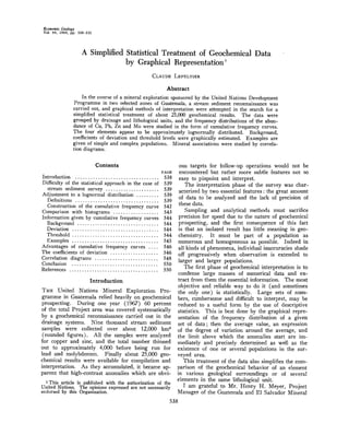
11. 548 CLAUDE LEPELTIER
Figure7. CorrelationdiagramCu/Zn
cu(pp,.) •
III • ßIII
ß IllIll / ' x .,
Ill , / X , Ill
Ill I " • Ill
III , ,,,
Cu :
ß. - Il
/' • I II
Ill .... :-_ . tll•III
'.A......• • • Ill,,i
III Jill
III ...............', IIII II
III ; •11
Ill , III
III ill
5670910 2 3 4 5 67891• 2 3 4 5 67091ffi0
N1=nI +n3=168
In Figure 6, it is also interestingto note the
variationsof the dispersionof the sameelementin
different lithological units which is particularly
noticeablefor copper;the width of eachparallelo-
gram indicatesthe rangeof variationof s for each
element.
The coefficientof deviation is a very important
character of the distribution of an element in a
givensurrounding;it is probablyrelatedto the type
of geochemicaldispersion,mechanicalor chemical,
and consequentlymight give an indicationof the
type of anomalyencountered:syngeneticor epi-
genetic. It appearsthata highercoefficientof devi-
ationindicatesa preponderantlymechanicaldisper-
sion,but this hasnot beenproved. Much remains
to be done in this field.
Correlation Diagrams
In the caseof a polymetallicmineralization,with
two or moreelementslognormallydistributed,there
isgenerallya positivecorrelationbetweenthem;for
instancebetweenleadandzinc,a samplehighin Pb
iscommonlyalsohighin Zn. Thisgeologicconcept
of a relationshipbetweentwo-typesof mineralization
(onlyqualitativeandrathervague)maybe substi-
tutedby a precisefactor,the coefficientof correla-
tionp, whichgivesa rigorousmeasureof their de-
gree of dependency.In the caseof geochemical
prospecting,p measuresthedegreeof dependencyof
two lognormalvariablesnamelythe tenorsof two
elementsin a samplepopulation(Matheron,1962).
The coefficientpalwaysfallsbetween-1 and+ 1.
p--o meansa completeindependencebetweenthe
twoelements,p-- --+-1indicatesa functionalrelation-
ship,director inverse,betweenthem(it is a linear
relationshipbetweenthe logarithmsof the tenors).
SimplifiedCalculationof p.--Thereis a graphical
way to estimatep, slightlylessprecisebut much
fasterthan the completestatisticalcalculation:con-
structinga correlationcloudin full log.coordinates
(Fig. 7, 8). Eachsampleof thepopulationunder
studyis plottedfollowingits t•vo coordinates:its
tenor in element •/ and its tenor in element B and
the totalpopulationappearsas a cloudof points.
13. 550 CL,ZIUDE LEPELTIER
may be usedto assessmineralassociationsof ele-
mentsin naturalsamples. The correlationdiagram
showswhethertwo elementsare spatiallyassociated
andif onemaybeusedasa pathfinderfor theother.
Let us considertwo examples'the relationshipof
Cu/Zn in the drainageof the SuchiateRiver (Fig.
7) andtherelationshipof Pb/Zn in theRio Grande
drainage(Fig. 8).
Thefirstexample,in Figure7, isintendedonlyto
illustrate the lack of relationshipbetweentwo types
ofmineralization.The cloudofpointshasnodefinite
shape,but it canbe dividedinto threezones'one
aroundthe intersectionpointof the axes,including
the majorityof the pointswhichare spreadmore
orlessequallyamongthefourquadrants;anelliptical
one,markedCu, in therangehigh-Cu/background-
Zn values;and a third one, includingonly a fe•v
high-Zn/background-Cupoints.Thisshowsthat,in
the Suchiatedrainage,thereis norelationshipwhat-
soever between the Cu and Zn mineralization, that
theCu anomalyis moreimportantthanthatfor Zn
and that the two anomaliesare well separated
spatially.All thisisexpressedbythecoefficientof
correlation'
p = -0.11
Its low absolutevalue indicatesa nearlycomplete
independenceof the two mineralizations,with a
tendency'to inverserelationship(negativevalue).
On thecontrary,Figure8 showsan exampleof
directrelationshipbetweentwotypesof mineraliza-
tion. In the Rio Grande drainage,Pb and Zn are
associated'the correlation cloud is an elongated
ellipsewhosemainaxishasa 45ø slopeandthe
correlationcoefficientt•---+0.87. In thisdrainage,
lead and zinc anomalies will have the same pattern
andwill bespatiallyrelated.In similargeological
conditions,oneelementmaybeusedasa pathfinder
for the other.
Conclusion
In theGuatemalangeochemicalreconnaissance,the
statisticalanalysisof thedata,althoughelementary,
was usefulin outliningsubduedanomalouspatterns
in a complexgeochemicalsurrounding,but much
moreinformationcancertainlybe extractedfrom the
analytical results by a more thorough, computer-
oriented, treatment.
The graphicalmethodsdescribedabovehave the
great advantageof beingquick,cheapand easyto
use in the field without any specialmathematical
knowledge. It is a convenientand syntheticway
to presenta greatamountof geochemicaldata,and
I think it mightbe usefulto any geologistinvolved
in geochemicalprospecting.
UNITED NATIONS MINERAL SURVEY,
GUATEMALACITY, GUATEMALA,
January20; March 28,1969
REFERENCES
Ahrens,L. H., 1957,The lognormaldistributionof the
elements--a fundamental law of geochemistry: Geochim.
et Cosmochim. Acta, v. 11, no. 4.
Coulomb,R., 1959,Contribution3,la C•ochimiede l'uranium
dansles granitesintrusifs:RapportC.E.A. 1173,Centre
d'EtudesNucleires de Saclay, France.
Cousins,C. A., 1956,The value distributionof economic
minerals with special referenceto the Witwatersrand
Gold Reefs: Geol. Soc. South Africa Trans. v. LIX.
Hubaux,A., 1961,Representationgraphiquedesdistributions
d'oligo-•l•ments:Ann.Soc.G•ol.Belgique,T. LXXXIV--
Mars 1961.
Termant,C. B., andWhite, M. L., 1959,Studyof the dis-
tribution of somegeochemicaldata: ECON.GEOL.,V. 54,
p. 1281--1290.
Matheron,G., 1962,Trait• de g•ostatistiqueappliqu•e,tome
1: M•moire no. 14 du Bureau de RecherchesG•ologiques
et MiniSres, Paris.
Miesh,A. T., 1967,Methodsof computationfor estimating
geochemicalabundance--U. S. GeologicalSurvey Pro-
fessionalPaper 574-B.
Monjallon,A., 1963,Introduction3. la m•thodestatistique:
Vuibert, Paris.
Rodionov,D. A., 1965,Distributionfunctionsof the elements
and mineral contentsof igneousrocks: ConsultantBureau,
New York.
Shaw,D. M., 1964,Interpretationg•ochimiquedes•l•ments
en trace dans les roches cristallines: Masson et Cie,
Paris.
Vistelius,A. B., 1960,The skewfrequencydistributionsand
fundamentallaw of the geochemicalprocesses:Journal of
Geol. Jan. 1960.