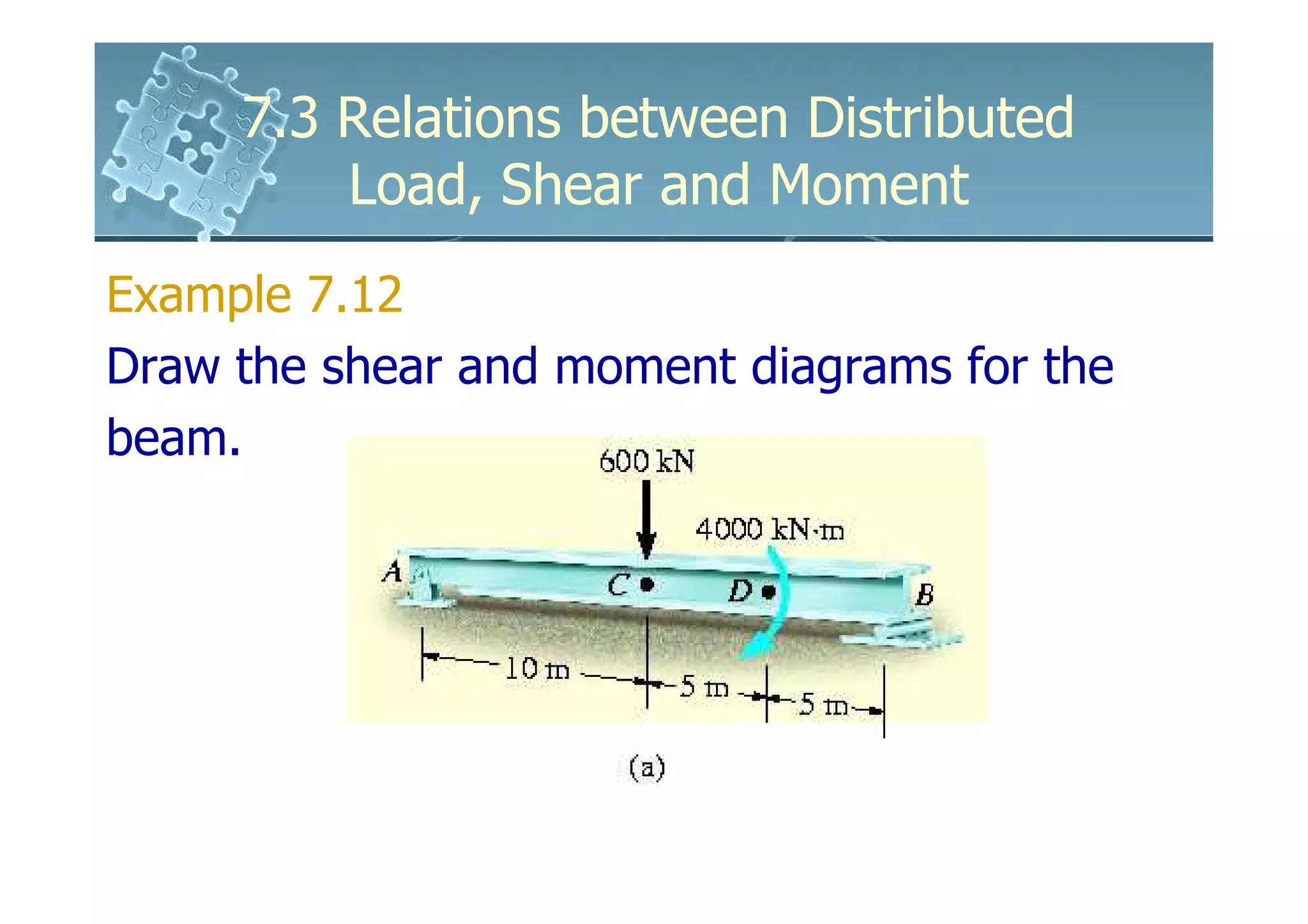
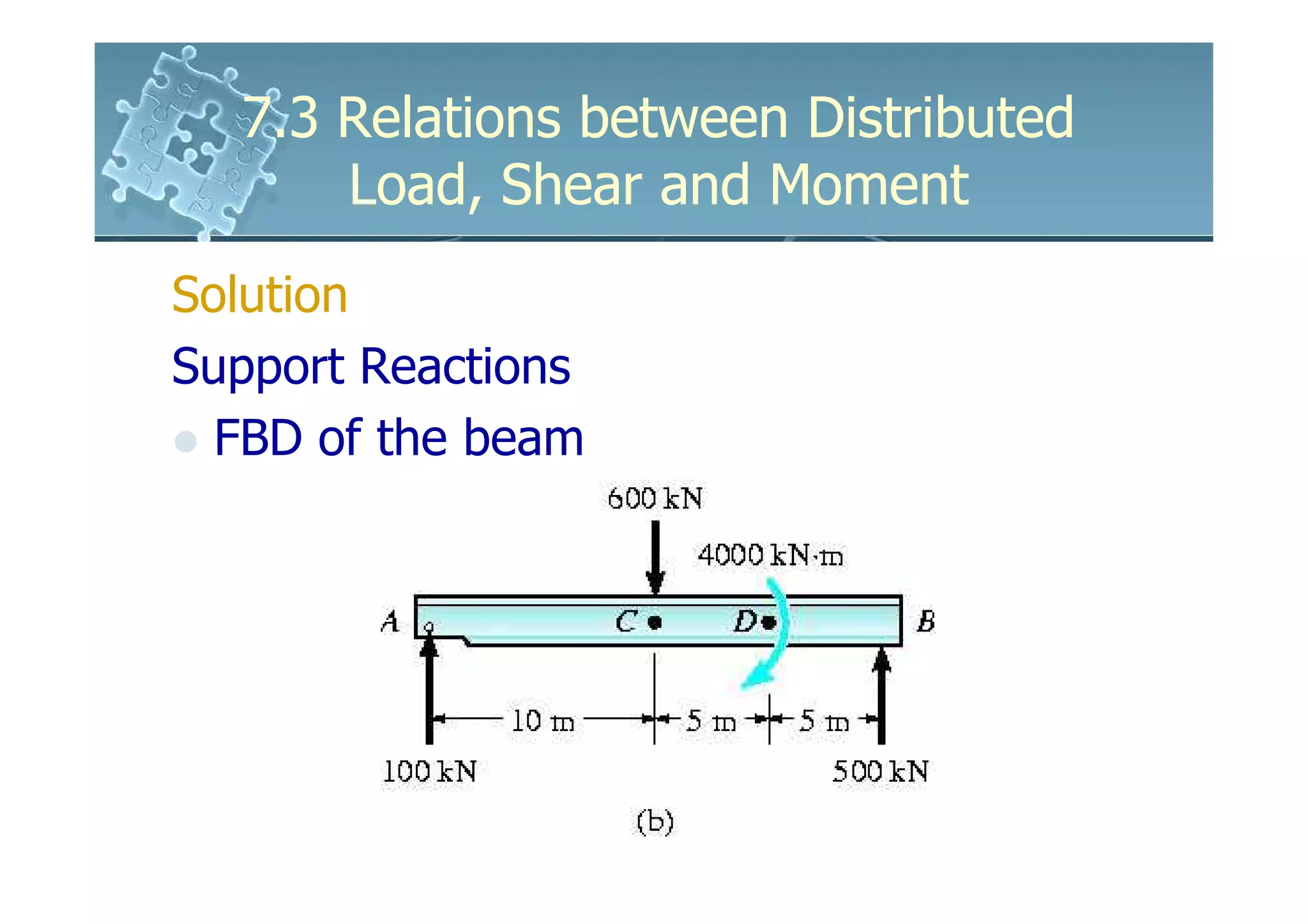
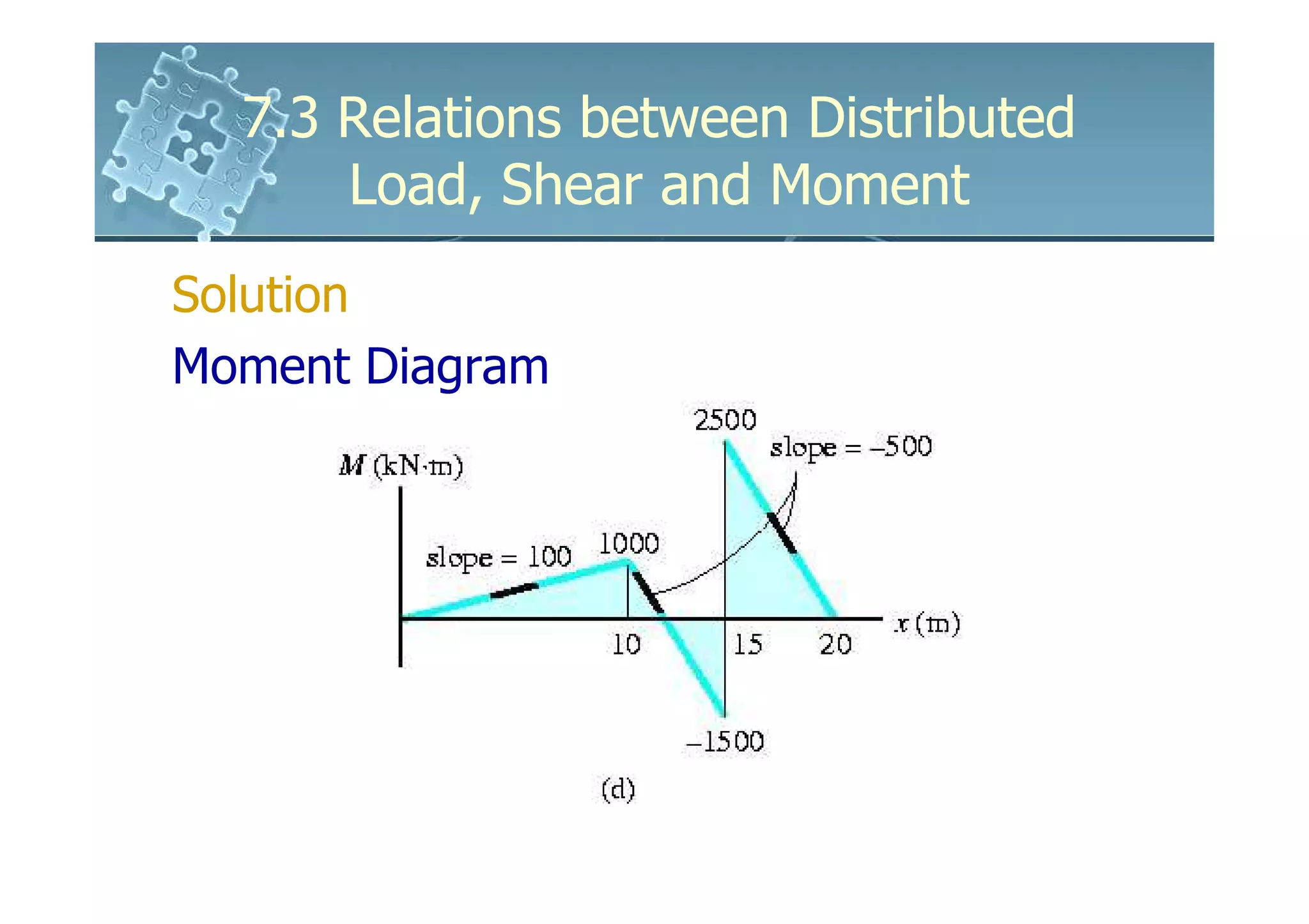
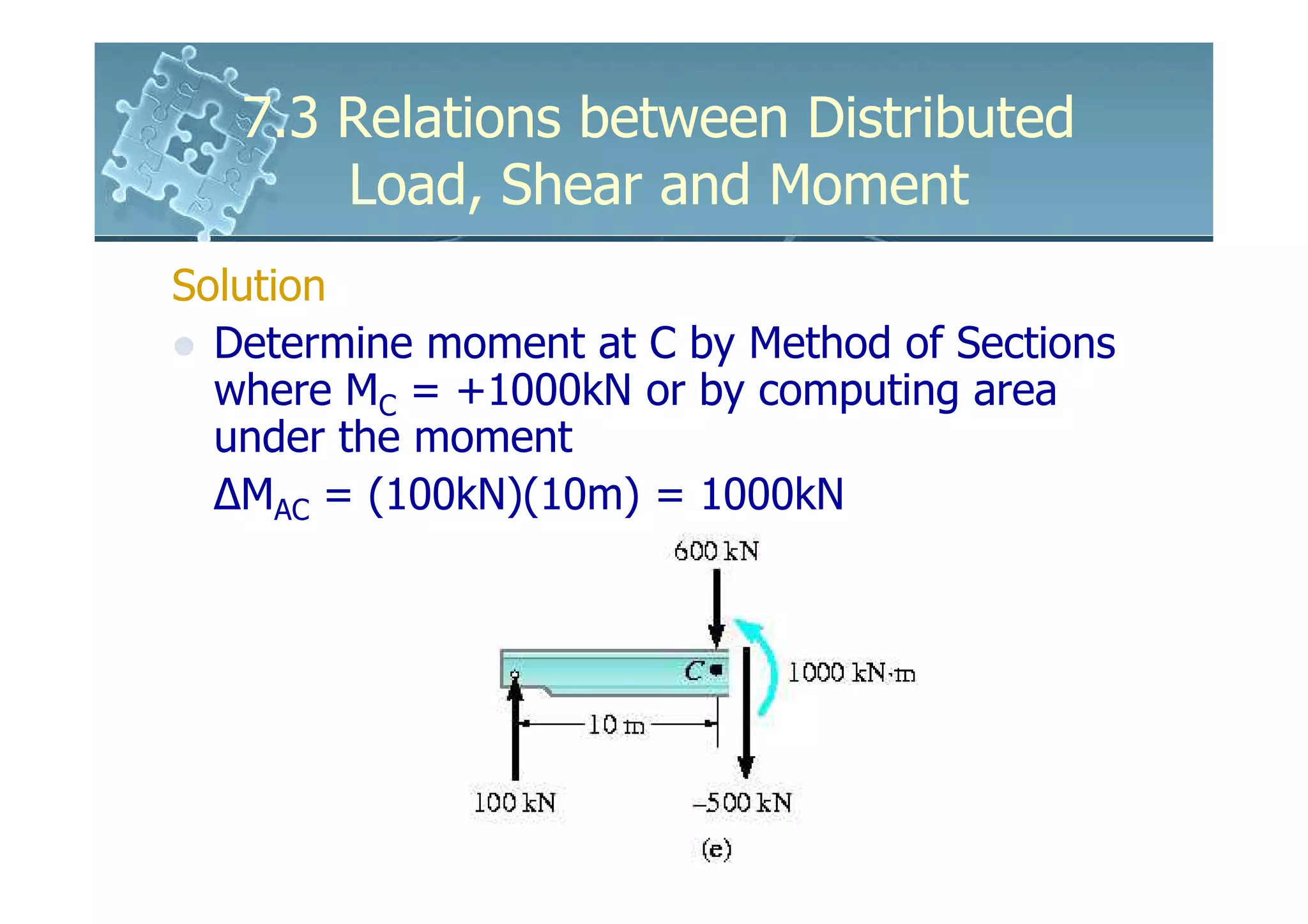
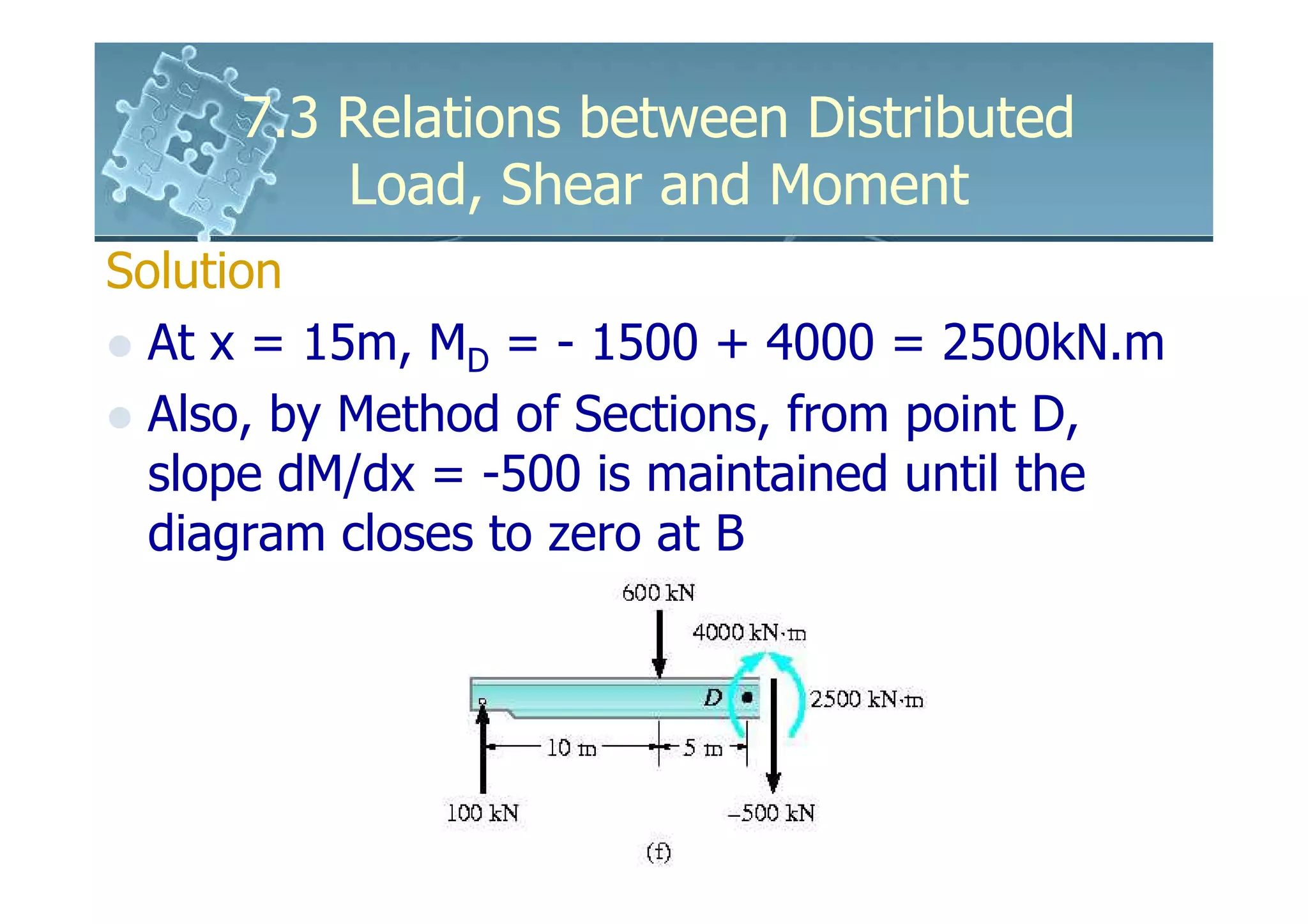
1) The document discusses the relationships between distributed loads, shear forces, and bending moments in beams.
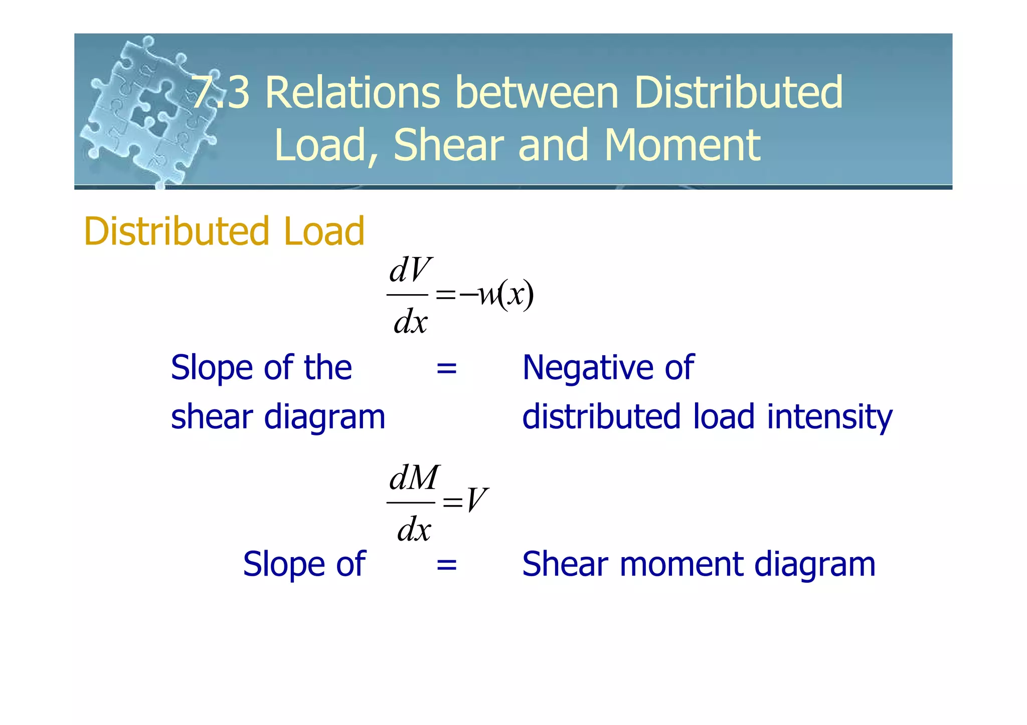
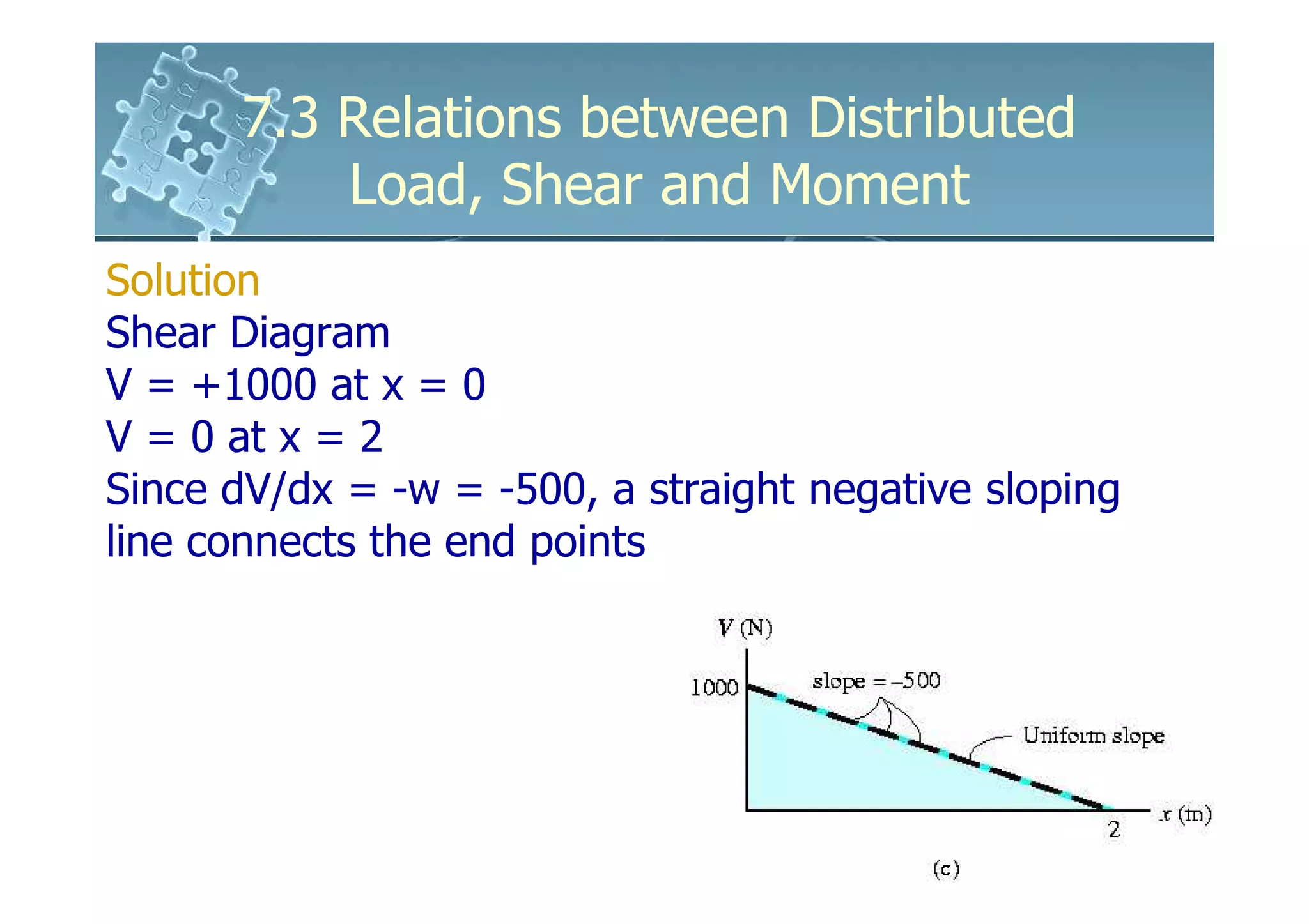
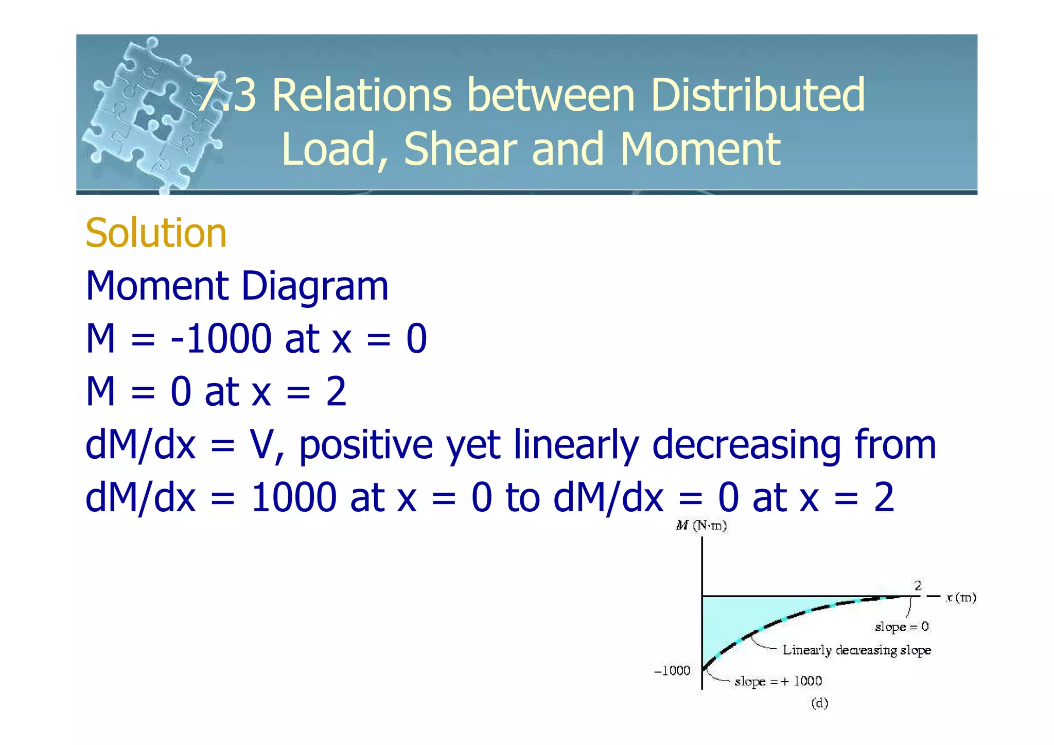
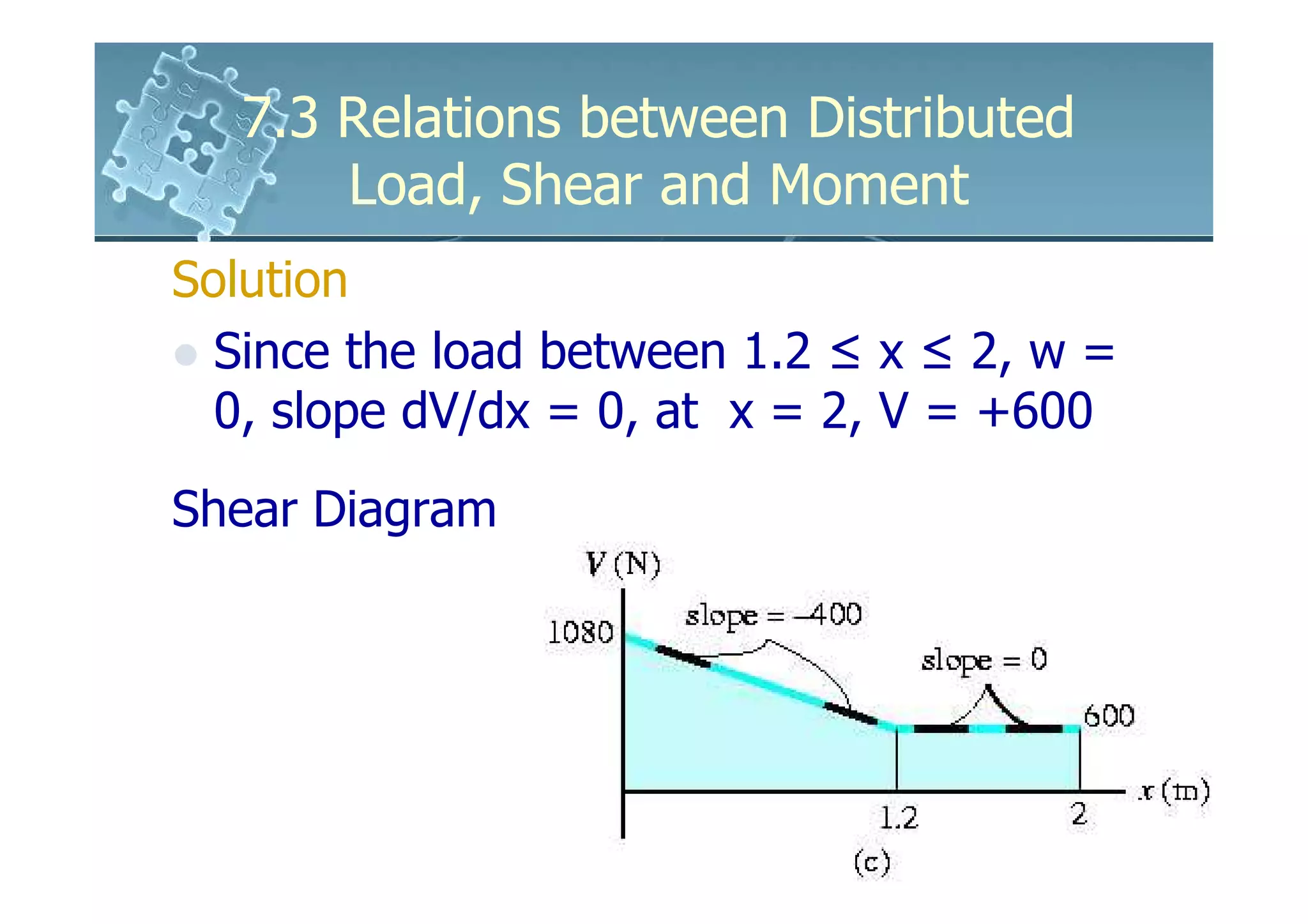
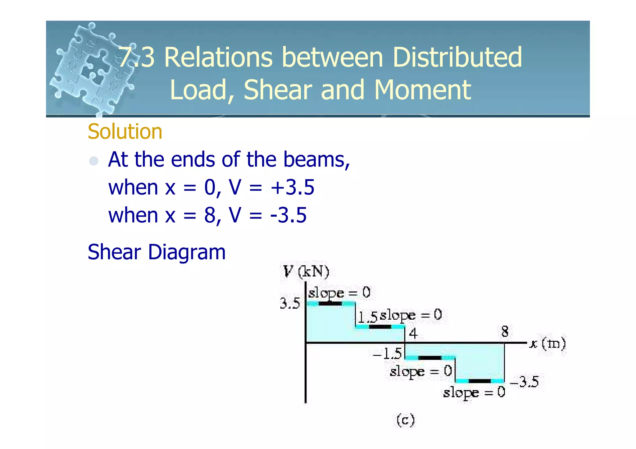
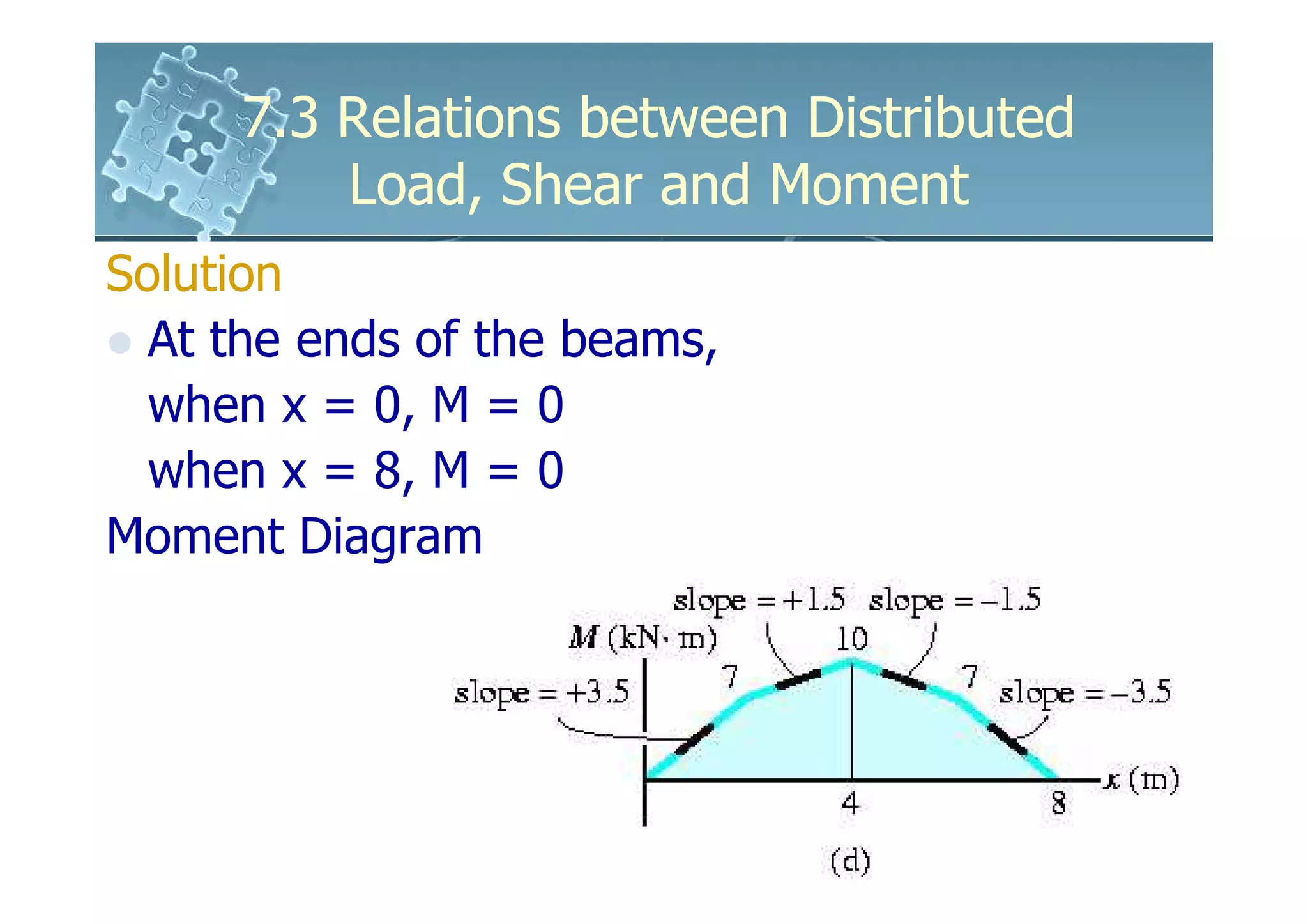
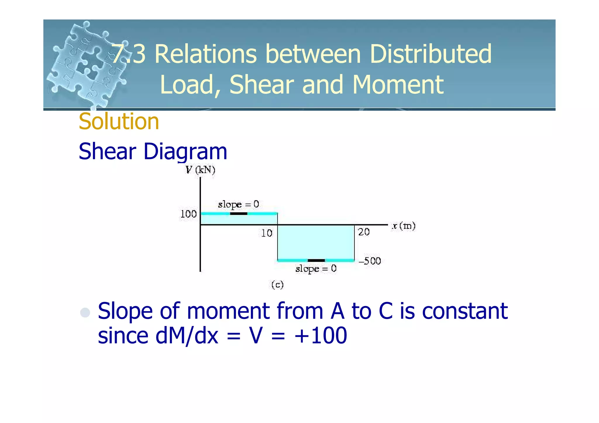
2) It shows that the slope of the shear diagram is equal to the distributed load intensity, and the slope of the moment diagram is equal to the shear force.
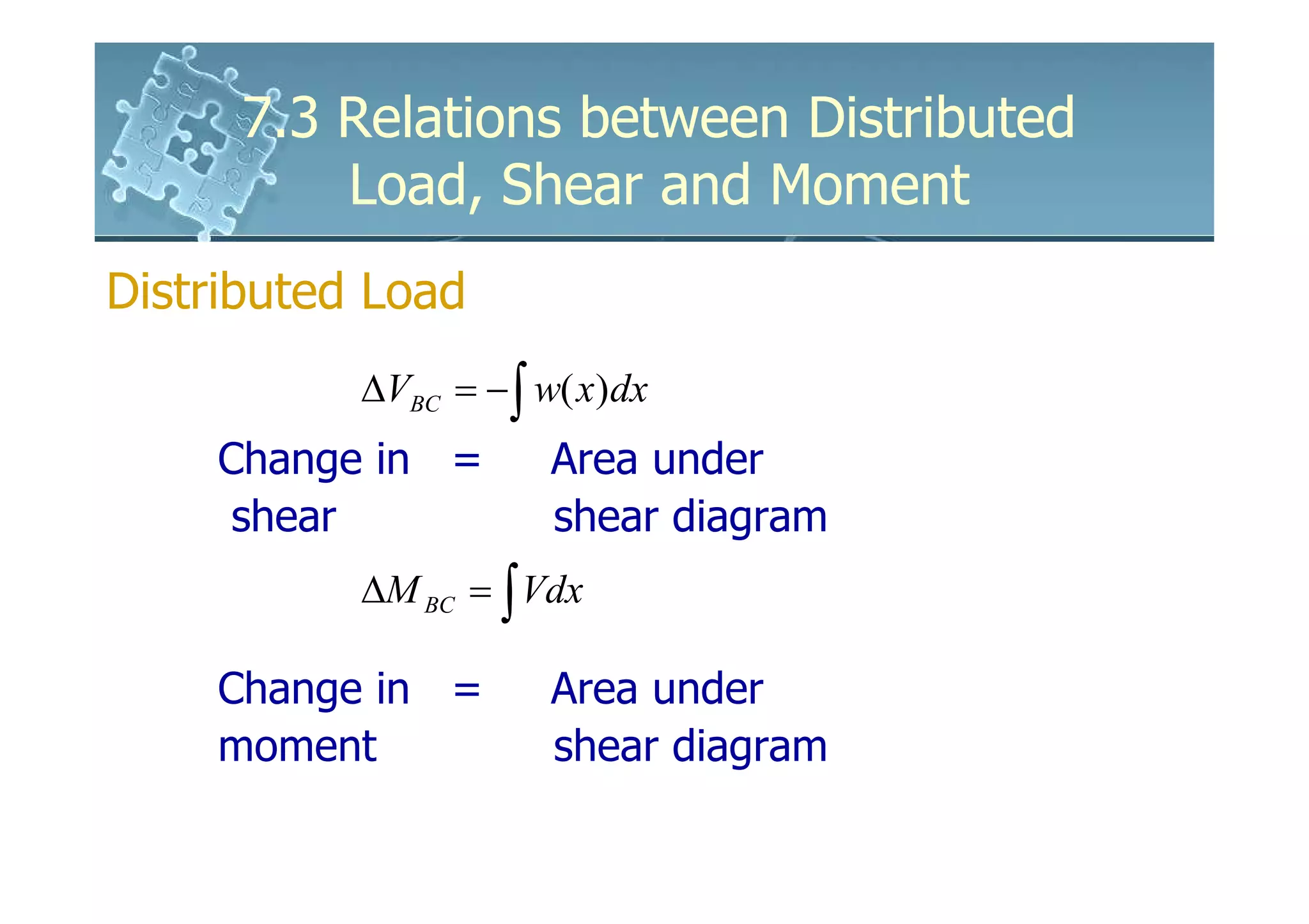
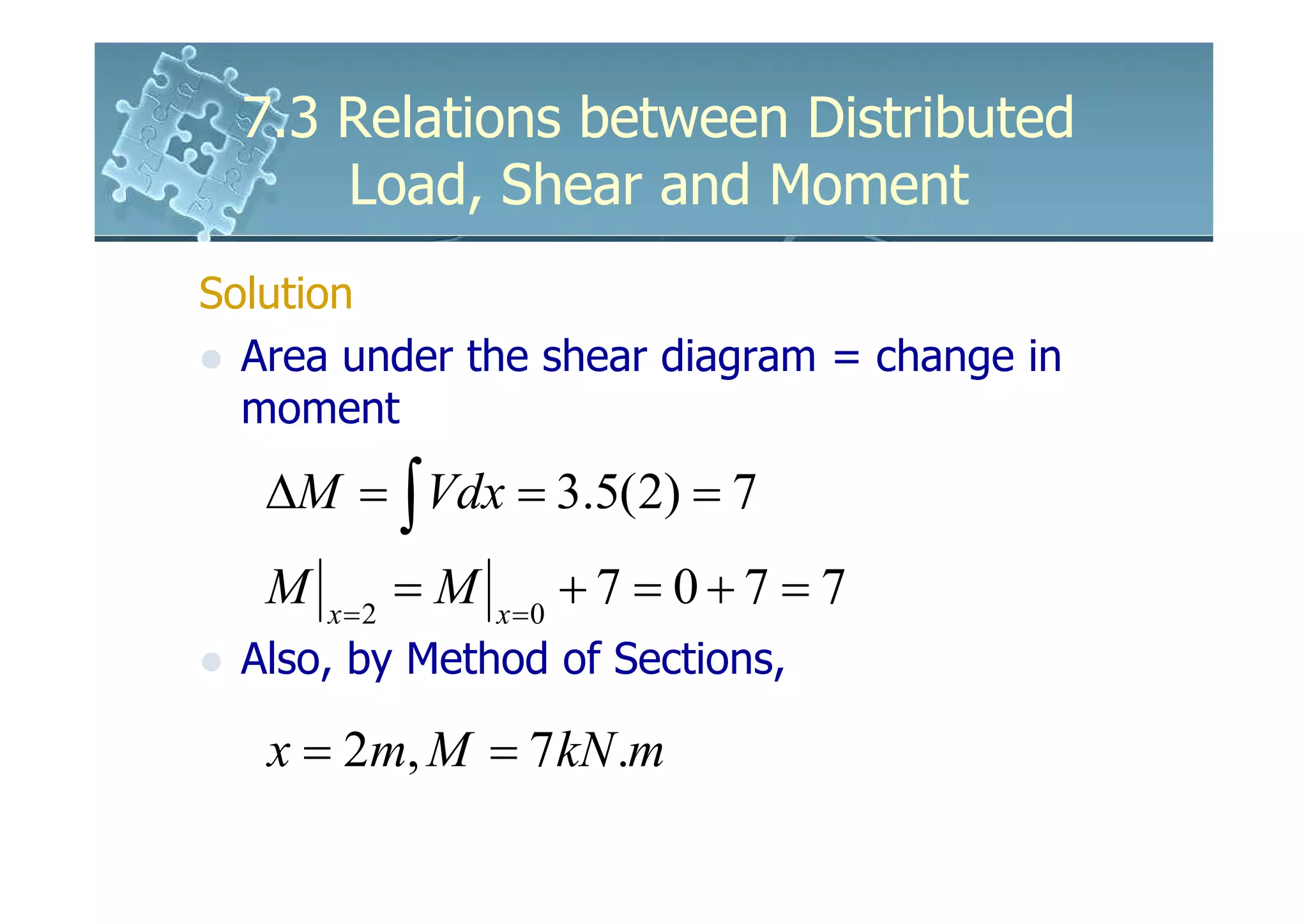
3) The change in shear force between two points is equal to the negative area under the distributed load diagram between those points. The change in bending moment is equal to the area under the shear diagram.
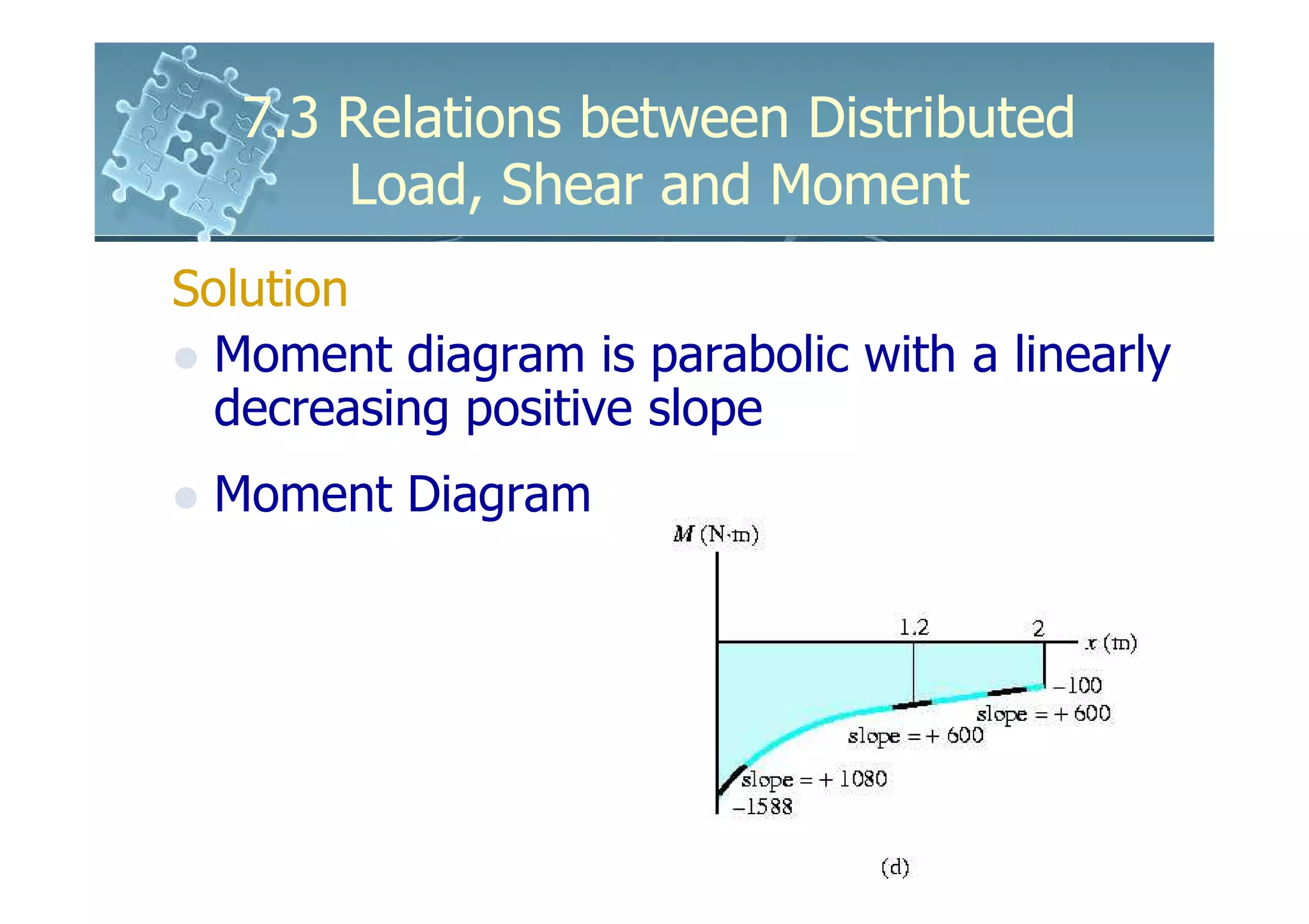
![7.3 Relations between Distributed
Load, Shear and Moment
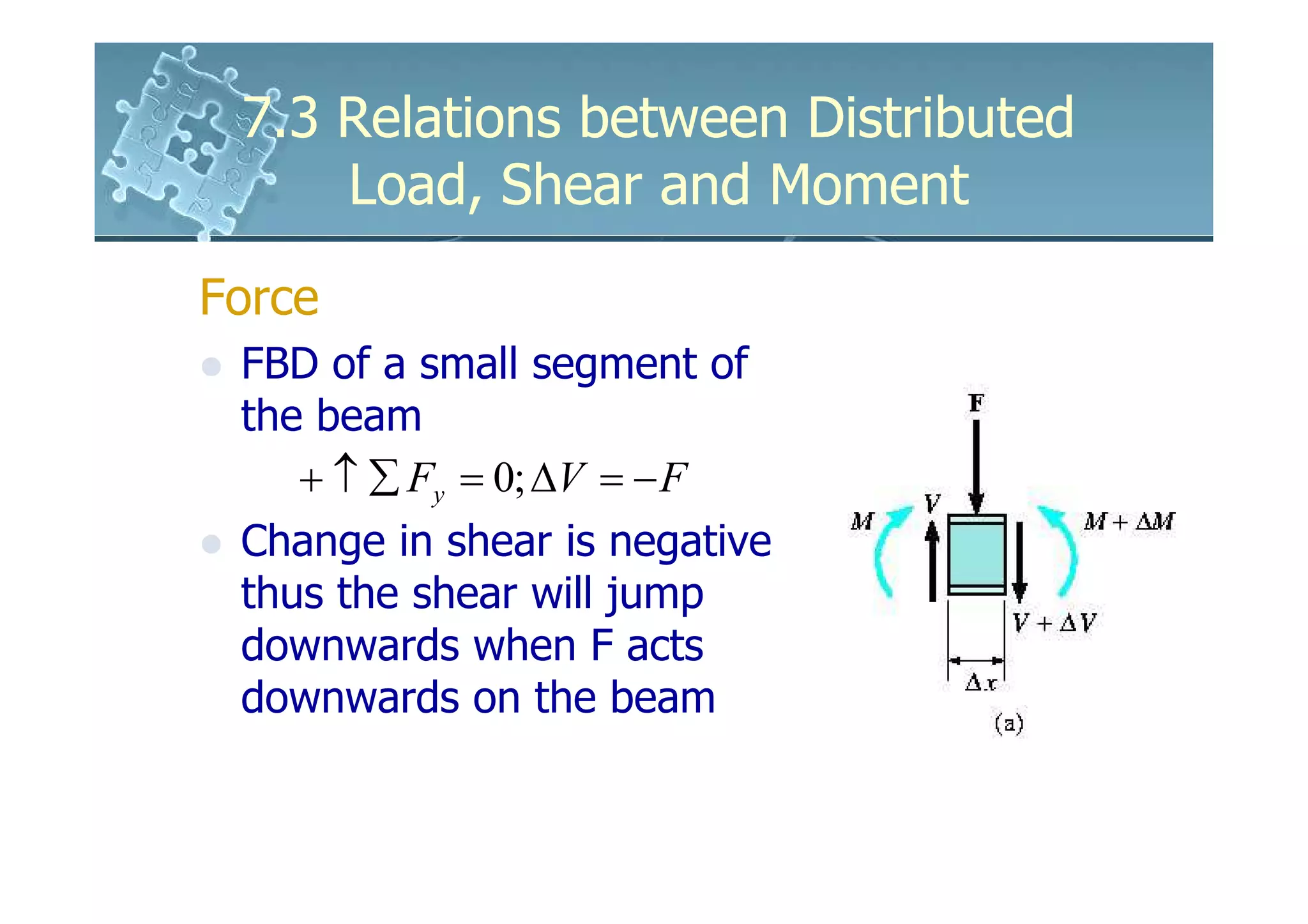
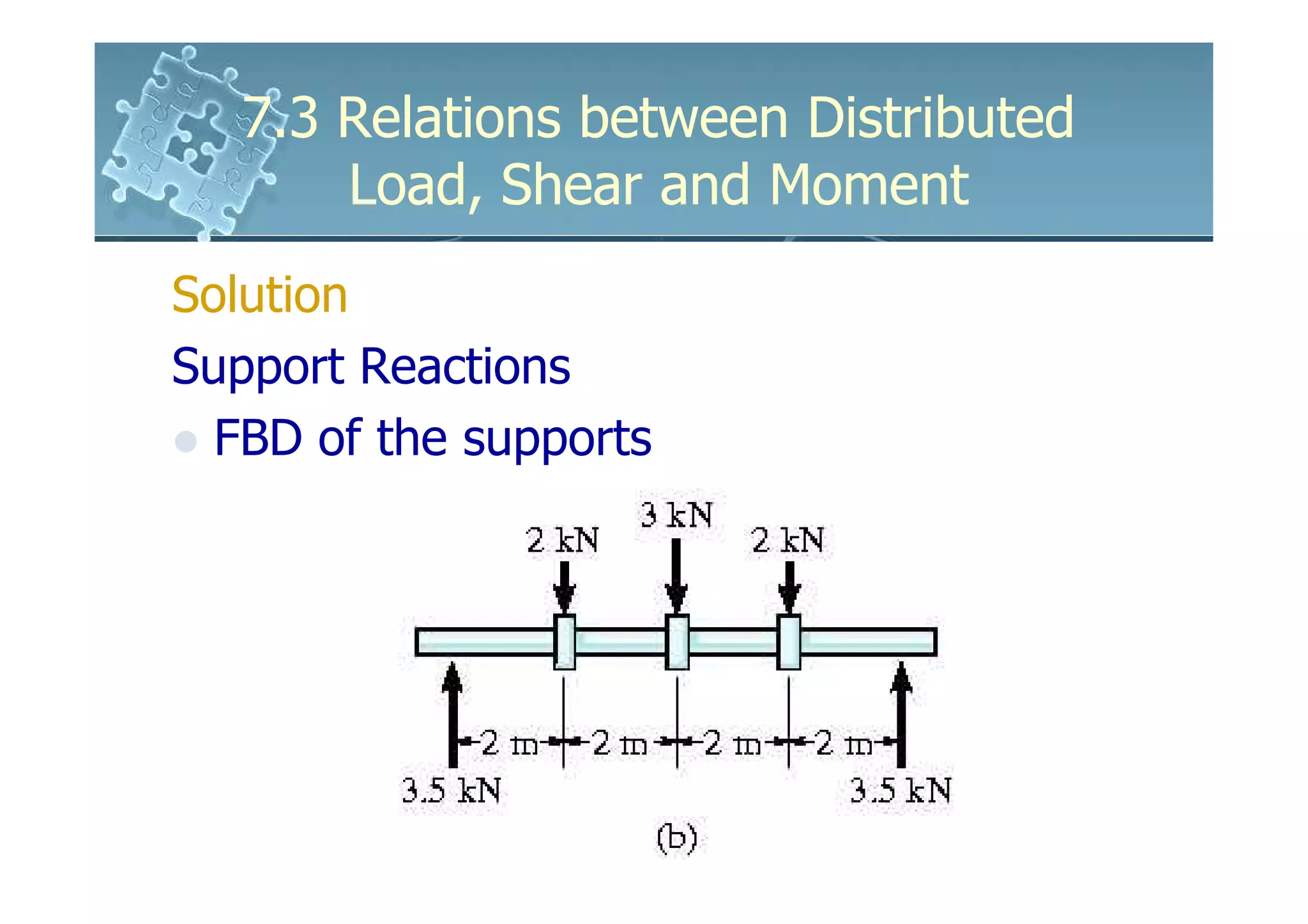
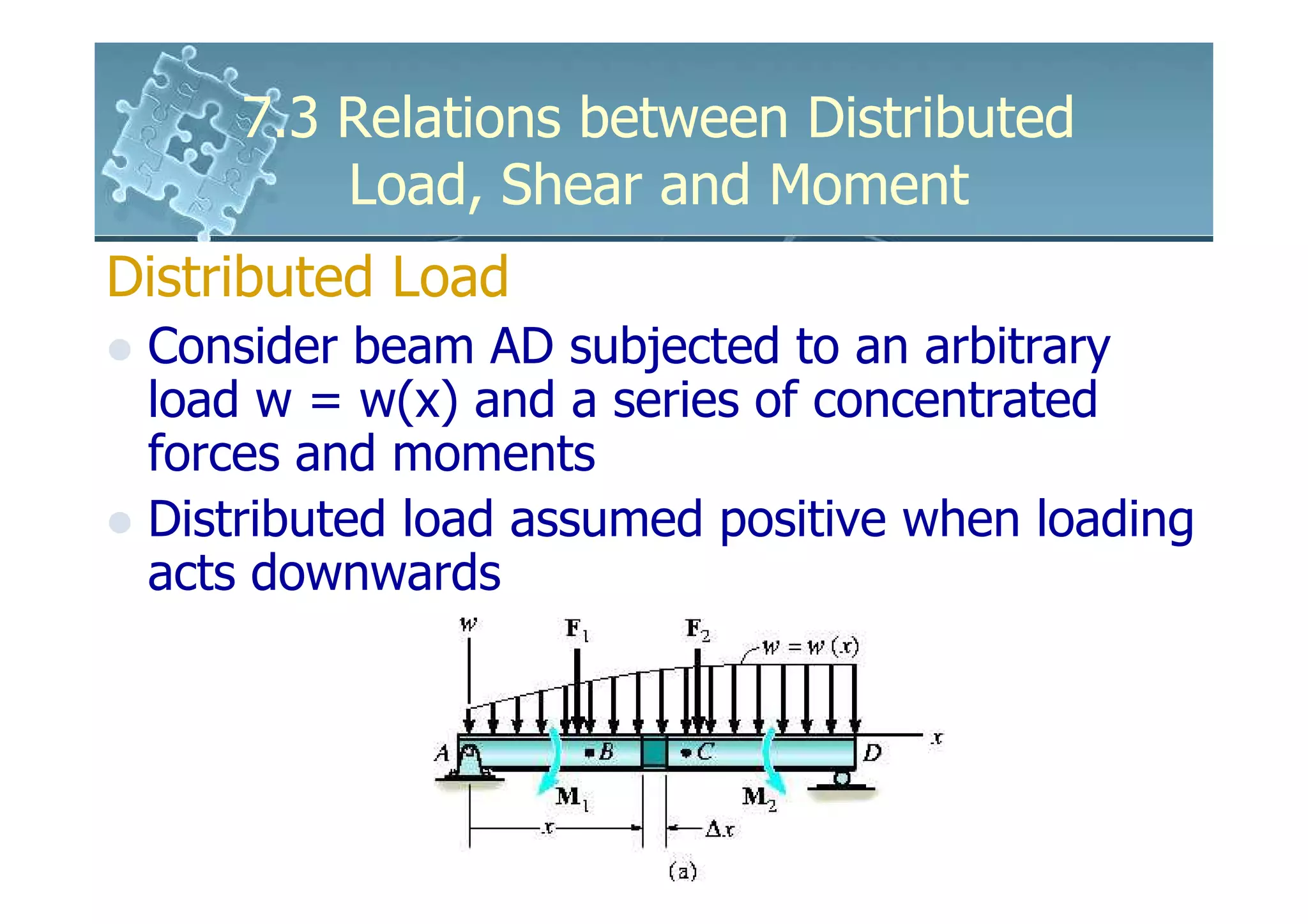
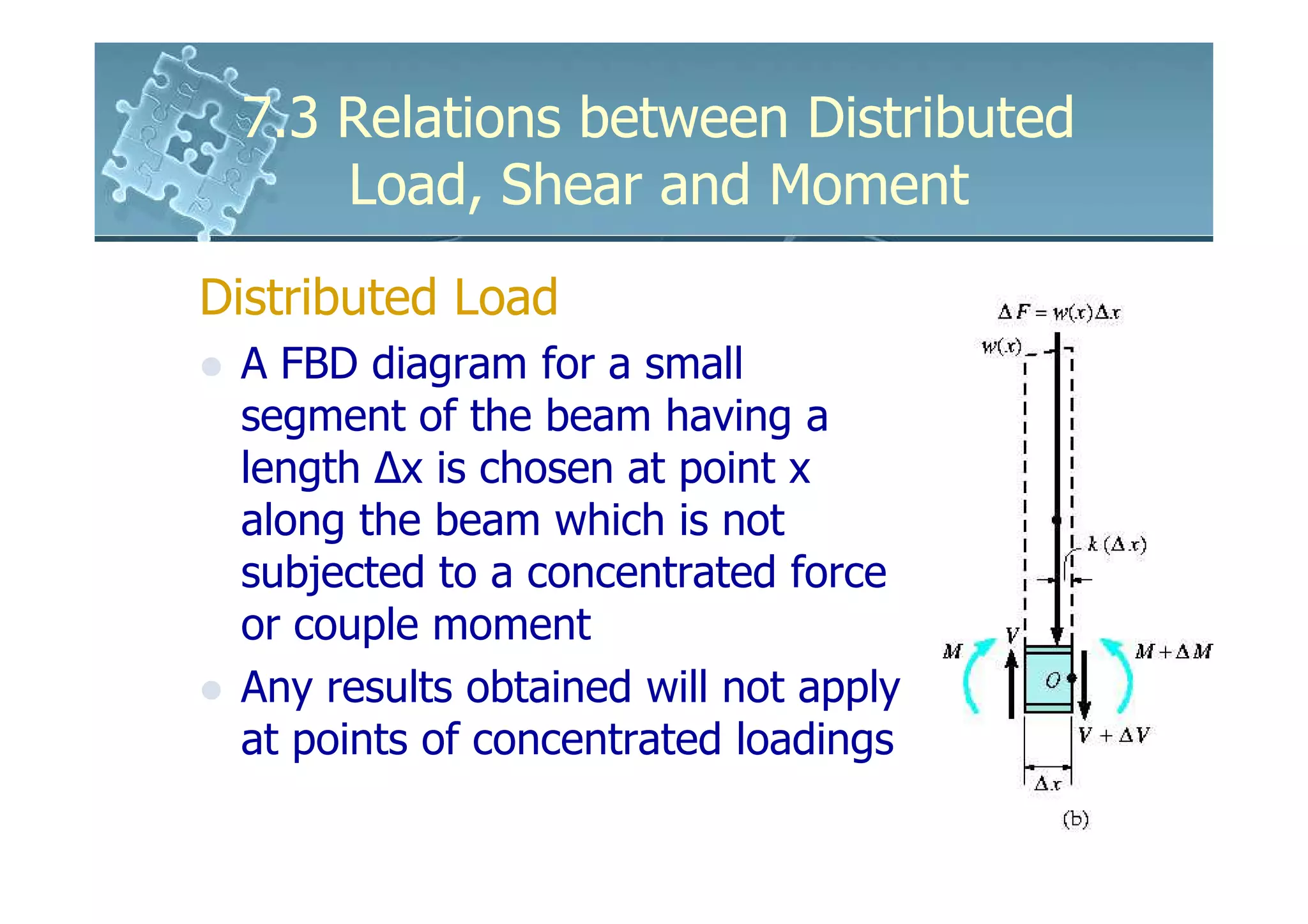
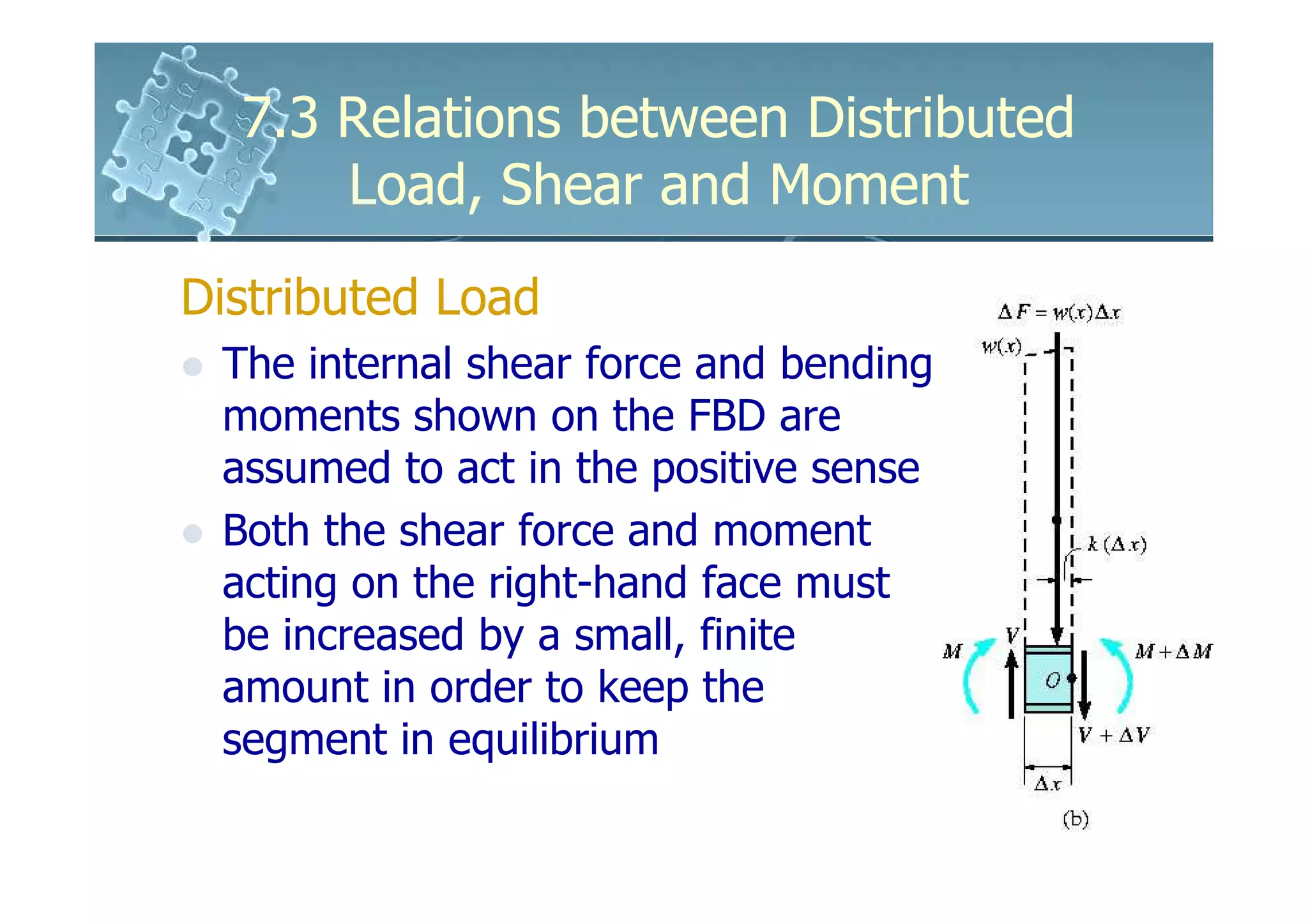
Distributed Load
The distributed loading has been replaced by a
resultant force ∆F = w(x) ∆x that acts at a
fractional distance k (∆x) from the right end,
where 0 < k <1
+ ↑ ∑ Fy = 0;V − w( x)∆x − (V + ∆V ) = 0
∆V = − w( x)∆x
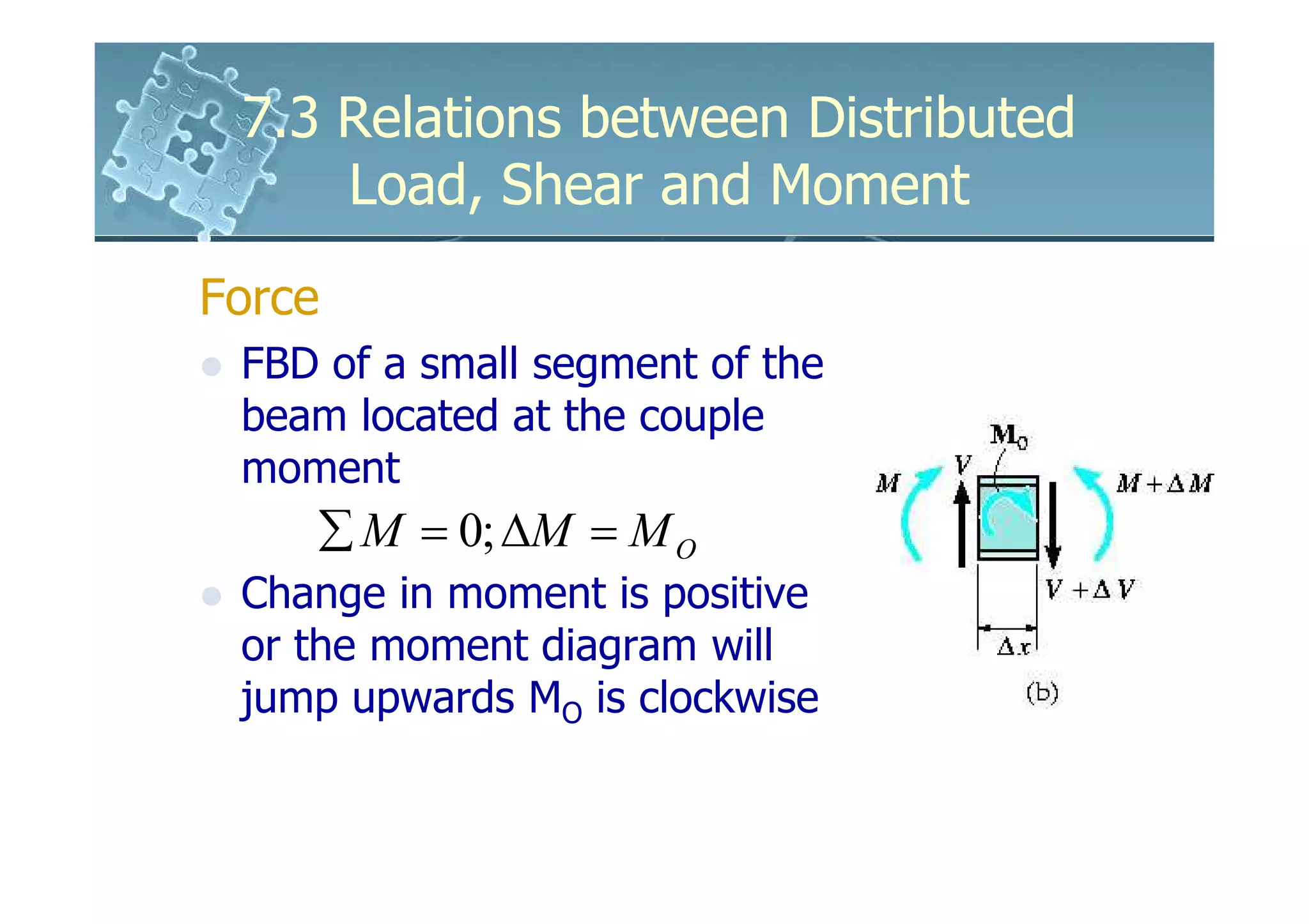
∑ M = 0;−V∆x − M + w( x)∆x[k (∆x )] + ( M + ∆M ) = 0
∆M = V∆x − w( x)k (∆x) 2](https://image.slidesharecdn.com/61611037-3relationsbetweendistributedloadshearandmoment-120122212826-phpapp01/75/6161103-7-3-relations-between-distributed-load-shear-and-moment-4-2048.jpg)