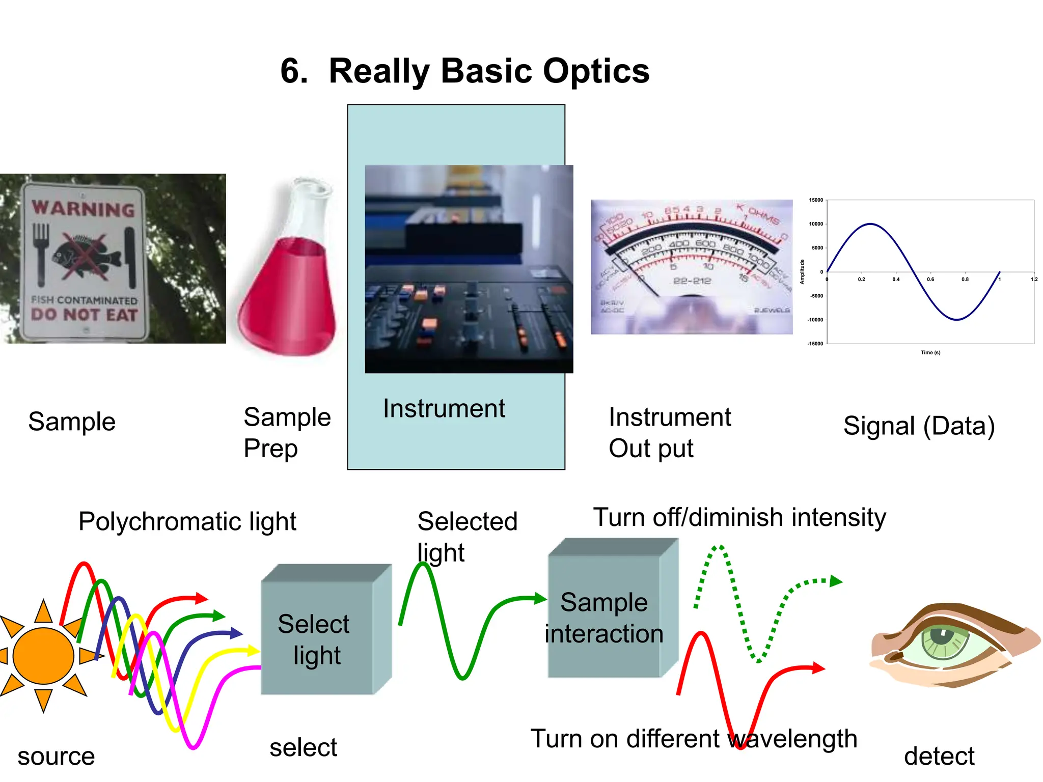
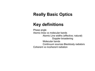
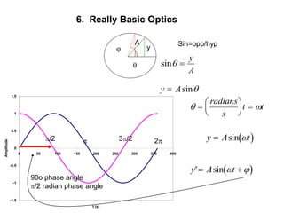
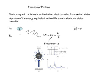
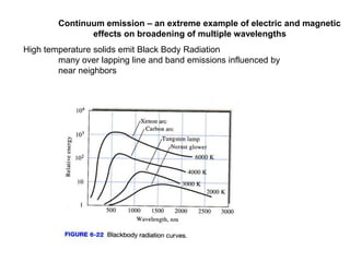
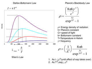
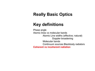
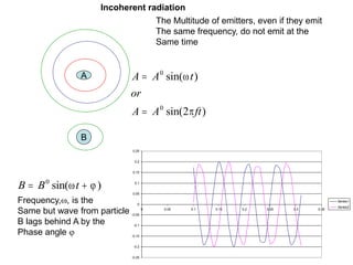
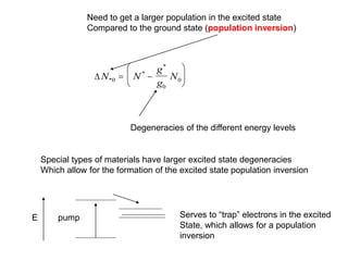
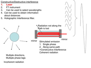
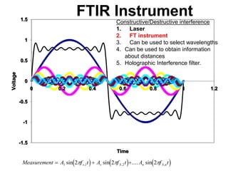
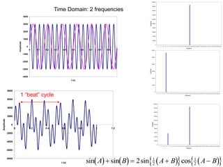
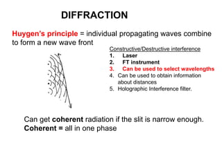
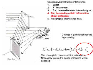
SlideShare a Scribd company logo
6. Really Basic Optics
-15000
-10000
-5000
0
5000
10000
15000
0 0.2 0.4 0.6 0.8 1 1.2
Time (s)
Amplitude
Sample Sample
Prep
Instrument Instrument
Out put
Signal (Data)
Select
light
Sample
interaction
source select
Turn off/diminish intensity
detect
Polychromatic light Selected
light
Turn on different wavelength
Really Basic Optics
Key definitions
Phase angle
Atomic lines vs molecular bands
Atomic Line widths (effective; natural)
Doppler broadening
Molecular bands
Continuum sources Blackbody radiators
Coherent vs incoherent radiation
6. Really Basic Optics
y

Sin=opp/hyp
sin 
y
A
y A
 sin
A

 






 
radians
s
t t
 
y A t
 sin 
 
y A t
' sin
 
 
-1.5
-1
-0.5
0
0.5
1
1.5
0 50 100 150 200 250 300 350 400
t (s)
Amplitude
90o phase angle
/2 radian phase angle
/2  3/2 2
Emission of Photons
Electromagnetic radiation is emitted when electrons relax from excited states.
A photon of the energy equivalent to the difference in electronic states
Is emitted
e
E h
hc
 


Ehi
Elo
Frequency 1/s
  c
Really Basic Optics
Key definitions
Phase angle
Atomic lines vs molecular bands
Atomic Line widths (effective; natural)
Doppler broadening
Molecular bands
Continuum sources Blackbody radiators
Coherent vs incoherent radiation
Theoretical width of an atomic spectral line
Line broadens due
1. Uncertainty
2. Doppler effect
3. Pressure
4. Electric and magnetic fields
 
 t  1
Lifetime of an excited state is typically 1x10⁻⁸ s
  

1
10
5 10
1
8
7
s
x
s
 
 
c 1
d
d
c



  
1 2
d
c
d





2







c c

 
2
2
Natural Line Widths
frequency
 


























5 10
1
3 10
10
5 10
7 2
8
9
10
2
x
s
x
m
s
nm
m
x
nm


Example: 253.7 nm
 
 





 


5 10
2537 322 10
10
2 5
x
nm
nm x nm
. .
Typical natural line widths are 10-5 nm



0

elocity
c
Line broadens due
1. Uncertainty
2. Doppler effect
3. Pressure
4. Electric and magnetic fields
Line broadens due
1. Uncertainty
2. Doppler effect
3. Pressure
4. Electric and magnetic fields
The lifetime of a spectral event is 1x10⁻⁸ s
When an excited state atom is hit with another high energy atom
energy is transferred which changes the energy of the
excited state and, hence, the energy of the photon emitted.
This results in linewidth broadening.
The broadening is Lorentzian in shape.
 
f
FWHM
FWHM
o
( )


  




















1 2
2
2
2
FWHM = full width half maximum
o is the peak “center” in frequency units
We use pressure broadening
On purpose to get a large
Line width in AA for some
Forms of background
correction
Line spectra – occur when radiating species are atomic particles which
Experience no near neighbor interactions
Overlapping line spectra lead to band emission
Line broadens due
1. Uncertainty
2. Doppler effect
3. Pressure
4. Electric and magnetic fields
Line events
Can lie on top
Of band events
Continuum emission – an extreme example of electric and magnetic
effects on broadening of multiple wavelengths
High temperature solids emit Black Body Radiation
many over lapping line and band emissions influenced by
near neighbors
0 500 1000 1500 2000 2500 3000 3500
nm
Intensity
I T
  4
Wien’s Law
 max 
b
T
Stefan-Boltzmann Law

 









8
1
3
3
h
c
h
kT
exp
= Energy density of radiation
h= Planck’s constant
C= speed of light
k= Boltzmann constant
T=Temperature in Kelvin
= frequency












1 8
1
3
h
hc
kT
exp
1. As  ↓(until effect of exp takes over)
2. As T,exp↓, 
Planck’s Blackbody Law
Really Basic Optics
Key definitions
Phase angle
Atomic lines vs molecular bands
Atomic Line widths (effective; natural)
Doppler broadening
Molecular bands
Continuum sources Blackbody radiators
Coherent vs incoherent radiation
A
B
The Multitude of emitters, even if they emit
The same frequency, do not emit at the
Same time
Incoherent radiation
-0.25
-0.2
-0.15
-0.1
-0.05
0
0.05
0.1
0.15
0.2
0.25
0 0.05 0.1 0.15 0.2 0.25 0.3 0.35
Series1
Series2
A A t
or
A A ft


0
0
2
sin( )
sin( )


B B t
 
0
sin( )
 
Frequency,, is the
Same but wave from particle
B lags behind A by the
Phase angle 
Begin
Using Constructive and Destructive
Interference patterns based on phase lag
By manipulating the path length can cause an originally coherent beam
(all in phase, same frequency) to come out of phase can accomplish
Many of the tasks we need to control light for our instruments
Constructive/Destructive interference
1. Laser
2. FT instrument
3. Can be used to obtain information
about distances
4. Interference filter.
5. Can be used to select wavelengths
END: Key Definitions
More Intense Radiation can be obtained by Coherent Radiation
Lasers
Beam exiting the cavity is in phase (Coherent) and therefore enhanced
In amplitude
Argument on the size of signals that follows is from Atkins, Phys. Chem. p. 459, 6th Ed
Photons can stimulate
Emission just as much
As they can stimulate
Absorption
(idea behind LASERs
Stimulated Emission)
*
o
Stimulated Emission
The rate of stimulated event is described by :
w B N
  *
 Is the energy density of radiation already present at the frequency of
the transition
B= empirical constant known as the Einstein coefficient for stimulated
absorption or emission
N* and No
are the populations of upper state and lower states
Where w =rate of stimulated emission or absorption
w B No
 
The more perturbing photons the greater the
Stimulated emission
Light Amplification by Stimulated Emission of Radiation
w B No
  w B N
  *

 









8
1
3
3
h
c
h
kT
exp
can be described by the Planck equation for black body radiation at some T

If the populations of * and o are the same the net absorption is zero as a photon is
Absorbed and one is emitted
In order to measure absorption it is required that the
Rate of stimulated absorption is greater than the
Rate of stimulated emission
w B N w B N
absorption o enussion
  
  *
N N
o  *
frequency
Need to get a larger population in the excited state
Compared to the ground state (population inversion)
N N
g
g
N
*0
*
*
 






0
0
Degeneracies of the different energy levels
Special types of materials have larger excited state degeneracies
Which allow for the formation of the excited state population inversion
Serves to “trap” electrons in the excited
State, which allows for a population
inversion
pump
E
Multiple directions,
Multiple phase lags
Stimulated emission
1. Single phase
2. Along same path
=Constructive Interference
Coherent radiation
Incoherent radiation
Radiation not along the
Path is lost
mirror
mirror
Constructive/Destructive interference
1. Laser
2. FT instrument
3. Can be used to select wavelengths
4. Can be used to obtain information
about distances
5. Holographic Interference filter.
-1.5
-1
-0.5
0
0.5
1
1.5
0 0.2 0.4 0.6 0.8 1 1.2
Time
Voltage
-1.5
-1
-0.5
0
0.5
1
1.5
0 0.2 0.4 0.6 0.8 1 1.2
Time
Voltage
-1.5
-1
-0.5
0
0.5
1
1.5
0 0.2 0.4 0.6 0.8 1 1.2
Time
Voltage
-1.5
-1
-0.5
0
0.5
1
1.5
0 0.2 0.4 0.6 0.8 1 1.2
Time
Voltage
-1.5
-1
-0.5
0
0.5
1
1.5
0 0.2 0.4 0.6 0.8 1 1.2
Time
Voltage
-1.5
-1
-0.5
0
0.5
1
1.5
0 0.2 0.4 0.6 0.8 1 1.2
Time
Voltage
-1.5
-1
-0.5
0
0.5
1
1.5
0 0.2 0.4 0.6 0.8 1 1.2
Time
Voltage FTIR Instrument
     
Measurement A f t A f t A f t
s s S n S n
  
1 1 2
2 2 2
sin sin .... sin
, , ,
  
Constructive/Destructive interference
1. Laser
2. FT instrument
3. Can be used to select wavelengths
4. Can be used to obtain information
about distances
5. Holographic Interference filter.
-4000
-3000
-2000
-1000
0
1000
2000
3000
4000
0 0.1 0.2 0.3 0.4 0.5 0.6 0.7 0.8 0.9 1
t (s)
Amplitude
Time Domain: 2 frequencies
0
20000
40000
60000
80000
100000
120000
140000
160000
180000
200000
1 2 3 4 5 6 7 8 9 10 11 12 13 14 15 16 17 18 19 20 21 22 23 24 25 26 27 28 29 30 31 32 33 34 35 36 37 38 39 40
frequency
amplitude
0
10000
20000
30000
40000
50000
60000
1 2 3 4 5 6 7 8 9 10 11 12 13 14 15 16 17 18 19 20 21 22 23 24 25 26 27 28 29 30 31 32 33 34 35 36 37 38 39 40
Frequency
Amplitude
-8000
-6000
-4000
-2000
0
2000
4000
6000
8000
0 0.2 0.4 0.6 0.8 1 1.2
t (s)
Amplitude
0
20000
40000
60000
80000
100000
120000
140000
160000
180000
200000
1 2 3 4 5 6 7 8 9 10 11 12 13 14 15 16 17 18 19 20 21 22 23 24 25 26 27 28 29 30 31 32 33 34 35 36 37 38 39 40
frequency
amplitude
1 “beat” cycle
     
   
 
sin sin sin cos
A B A B A B
   
2 1
2
1
2
Moving
mirror
IR source
Beam
splitter
Fixed mirror
B
C
A
detector
Constructive interference occurs when
AC BC n
 
1
2
 
-4000
-3000
-2000
-1000
0
1000
2000
3000
4000
Mirror distance
Light
Intensity
at
Detector
-2 -1 0 +1
 
dis ce f mirror velocity mirror
tan    
INTERFEROGRAMS


 
 
n
mirror
2 mirror mirror
velocity






 
n
mirror mirror
2
f
n
ector
mirror
det  
1 2



Remember that:



c
 f
cn
ector
mirror light
det
2 
Frequency of light
An interferometer detects a periodic wave with a
frequency of 1000 Hz when moving at a velocity of 1
mm/s. What is the frequency of light impinging on
the detector?
 f
cn
ector
mirror light
det
2 
No need to SELECT
Wavelength by using
Mirror, fiber optics,
Gratings, etc.
FOURIER TRANSFORMS
Advantages
1. Jaquinot or through-put
little photon loss; little loss of source intensity
2. Large number of wavelengths allows for ensemble averaging
(waveform averaging)
3. This leads to Fellget or multiplex advantage
multiple spectra in little time implies?
s
s
N
population samples
inite population
measurements

inf
S
N
x x
s
ignal
oise
sample blank
blank


 
S
N
N
s
x x
ignal
oise
measurements
inite population
sample blank
 
inf
S
N
N
ignal
oise
measurements

DIFFRACTION
Huygen’s principle = individual propagating waves combine
to form a new wave front
Can get coherent radiation if the slit is narrow enough.
Coherent = all in one phase
Constructive/Destructive interference
1. Laser
2. FT instrument
3. Can be used to select wavelengths
4. Can be used to obtain information
about distances
5. Holographic Interference filter.
June 19, 2008, Iowa Flood
Katrina Levee break
Fraunhaufer diffraction at a single slit
1 BD OD CD big assume
, , & , / /

2. / /,
if then BCF
  
9. sin sin
 
  
CBF
opposite
hypotenuse
CF
BC
DE
OD

7.  
EOD 
8.
( int )
CF must be n for in
phase constructive erference

10. sin
   






n CF BC
DE
OD
BC
 
4 90
. '
 
OF B o
3 180 90
.         
DEO EOD EOD
 
6 180 90
.         
CFB FBC BCF  
From which we conclude
11.  





 






n
DE
OD
BC
DE
OE
BC

12.  






n
d
L
W

C
B
F
F’
D
E
d
W L


O
5 90
. / /,
if then CFB o
 


The complete equation for a slit is
I I










0
2
sin
 
 

b
2
sin
0
0.2
0.4
0.6
0.8
1
1.2
-800 -600 -400 -200 0 200 400 600 800
Beta
Relative
Intensity
Width of the line depends upon
The slit width!!
Therefore resolution depends
On slit width
Also “see”
This spectra
“leak” of
Our hard won
intensity
B
D
E
d
W L

b=W/2
The base (I=0) occurs whenever
 
  
  
b
n
2
sin
0
0.2
0.4
0.6
0.8
1
1.2
-800 -600 -400 -200 0 200 400 600 800
Beta
Relative
Intensity
I I










0
2
sin sinβ =0
Which occurs when
line width n
b
W
W
   
2 2
2
2 2
2 2
   
sin sin sin
line width
W

2
sin
The smaller the
Slit width the
Smaller
The line width,
Which leads
To greater
Spectral
Resolution
Remember R is
Inversely proportional
To the width of
The Gaussian base
0
0.2
0.4
0.6
0.8
1
1.2
0 1 2 3 4 5 6
Image position
Output
of
detector
SLIT IMAGE
1 2 3
Image
1 2 3 4 5 Position number
Slit
When edge AB at Detector Sees
Position 1 0% power
Position 2 50% power
Position 3 100% power
Position 4 50% power
Position 5 0 % power
Detector output:
Triangle results when
Effective bandpass = image
To resolve two images that are ∆ apart requires
 
 
 2 eff
eff
Implies want a narrower slit
A
B
Essentially,
Narrow slit widths
Are generally better
 
 
 2 eff
GRATINGS
Gratings Groves/mm
UV/Vis 300/2000
IR 10/20
Points:
1. Master grating formed by diamond tip under ground
1. Or more recently formed from holographic processes
2. Copy gratings formed from resins
 
n CB BD
  
 
sin   
CAB
opp
hyp
CB
d
i q
  90
q
q
q CAB
   90
 
CAB i
sini
CB
d

 
sin   
DAB
opp
hyp
DB
d
r DBA
DBA BAD
DBA BAD
r BAD
  
    
   
 
90
90 180
90
sinr
DB
d

 
n CB BD
  
   
 
n d i d r
  
sin sin
   
 
n d i r
  
sin sin
+ -
EXAMPLE
Calculate  for a grating which has
i=45
2000 groves per mm
1) Get d
1
2000
500
mm
groves
nm
grove

2) Use grating equation to solve for     
 
n d i r
  
sin sin
   
 
n nm r
o
  
500 45
sin sin
Inputs that can be varied are in pink
d nlambda = d(sin+sinr)
grooves/mm 2000 500
i in degrees 45 0.785398 i in radians
r in degrees -40 -20 -10 0 10 20 40
radians -0.69813 -0.34907 -0.17453 0 0.174533 0.349066 0.698132
order n
1 32.15959 182.5433 266.7293 353.5534 440.3775 524.5635 674.9472
2 16.07979 91.27166 133.3647 176.7767 220.1887 262.2817 337.4736
3 10.71986 60.84777 88.90977 117.8511 146.7925 174.8545 224.9824
4 8.039896 45.63583 66.68233 88.38835 110.0944 131.1409 168.7368
5 6.431917 36.50866 53.34586 70.71068 88.0755 104.9127 134.9894
6 5.359931 30.42389 44.45488 58.92557 73.39625 87.42724 112.4912
Multiple wavelengths
Are observed
At a single angle
Of reflection!!
You get light of 674.9 nm
½; 1/3; 1/4; 1/5; etc.
Czerny-Turner
construction
440.3
220.1
146.8
88
73
All come
through
Physical Dimensions: 89.1 mm x 63.3 mm x 34.4 mm
Weight: 190 grams
Detector: Sony ILX511 linear silicon CCD array
Detector range: 200-1100 nm
Pixels: 2048 pixels
Pixel size: 14 μm x 200 μm
Pixel well depth: ~62,500 electrons
Sensitivity: 75 photons/count at 400 nm; 41 photons/count at 600 nm
Design: f/4, Symmetrical crossed Czerny-Turner
Focal length: 42 mm input; 68 mm output
Entrance aperture: 5, 10, 25, 50, 100 or 200 µm wide slits or fiber (no slit)
Grating options: 14 different gratings, UV through Shortwave NIR
Detector collection lens option: Yes, L2
OFLV filter options: OFLV-200-850; OFLV-350-1000
Other bench filter options: Longpass OF-1 filters
Collimating and focusing mirrors: Standard or SAG+
UV enhanced window: Yes, UV2
Fiber optic connector: SMA 905 to 0.22 numerical aperture single-strand optical fiber
Spectroscopic Wavelength range: Grating dependent
Optical resolution: ~0.3-10.0 nm FWHM
Signal-to-noise ratio: 250:1 (at full signal)
A/D resolution: 12 bit
Dark noise: 3.2 RMS counts
Dynamic range: 2 x 10^8 (system); 1300:1 for a single acquisition
Integration time: 3 ms to 65 seconds
Stray light: <0.05% at 600 nm; <0.10% at 435 nm
Corrected linearity: >99.8%
Electronics Power consumption: 90 mA @ 5 VDC
Data transfer speed: Full scans to memory every 13 ms with USB 2.0 or 1.1 port, 300 ms with serial port
Czerny-Turner
construction
440.3
220.1
146.8
88
73
All come
through
Ocean Optics
For fluorescence lab
Monochromator we looked inside
440.3
220.1
146.8
88
73
All come
through
440.3
Only
Hit grating first
Time to get
Hit grating second time
220.1 nm
Another way to look at it is to say
We Lose some of the light
Not all of it ends up at the intended angle of reflection
d nlambda = d(sin+sinr)
grooves/mm 2000 500
i in degrees 45 0.785398 i in radians
order 1 2 3 4 5
Reflection Angle
wavelength
100 -30.47131 -17.88496 -6.148561 5.330074 17.03125
125 -27.20057 -11.95286 2.458355 17.03125 32.88081
150 -24.02322 -6.148561 11.12168 29.53092 52.45672
175 -20.92262 -0.407192 20.05324 43.85957 #NUM!
200 -17.88496 5.330074 29.53092 63.23909 #NUM!
225 -14.89846 11.12168 40.0079 #NUM! #NUM!
250 -11.95286 17.03125 52.45672 #NUM! #NUM!
275 -9.039003 23.13464 70.54325 #NUM! #NUM!
300 -6.148561 29.53092 #NUM! #NUM! #NUM!
325 -3.273759 36.36259 #NUM! #NUM! #NUM!
350 -0.407192 43.85957 #NUM! #NUM! #NUM!
375 2.458355 52.45672 #NUM! #NUM! #NUM!
400 5.330074 63.23909 #NUM! #NUM! #NUM!
425 8.215299 83.16511 #NUM! #NUM! #NUM!
450 11.12168 #NUM! #NUM! #NUM! #NUM!
475 14.05736 #NUM! #NUM! #NUM! #NUM!
500 17.03125 #NUM! #NUM! #NUM! #NUM!
Light of 100
Nm shows up
At -30.4
AND
-17.88
And
-6.1
And
5.3
Etc.
GRATING DISPERSION
D-1 = Reciprocal linear dispersion
D
d
dy
dis ce between
dis ce on screen
d r
nF

  
1  
tan
tan
cos
Where n= order
F = focal length
d= distance/groove
D
d
nF
r

 
1
0
POINT = linear dispersion
What is (are) the wavelength(s) transmitted at 45o
reflected AND incident light for a grating of 4000
groves/mm?
RESOLUTION
The larger R the greater the spread between the two wavelengths, normalized by
The wavelength region
R nF

Where n = order and N = total grooves exposed to light
 
R ave




 
 


1 2
2 1
2


1 2
ave
What is the resolution of a grating in the first order
of 4000 groves/mm if 1 cm of the grating is
illuminated?
Are 489 and 489.2 nm resolved?
R nF

 
R ave




 
 


1 2
2 1
2

Change in path length results
In phase lag
     
 
E x y E x y ft x y
o
0 0 0
2
, , cos ,
 
 
The photo plate contains all the information
Necessary to give the depth perception when
decoded
Constructive/Destructive interference
1. Laser
2. FT instrument
3. Can be used to select wavelengths
4. Can be used to obtain information
about distances
5. Holographic Interference filter.
Interference Filter
Holographic Notch Filter
Constructive/Destructive interference
1. Laser
2. FT instrument
3. Can be used to obtain information
about distances
4. Interference filter.
5. Can be used to select wavelengths
Can create a filter using
The holographic principle
To create a series of
Groves on the surface
Of the filter. The grooves
Are very nearly perfect
In spacing
End
Section on Using Constructive
and Destructive
Interference patterns based on
phase lags
Constructive/Destructive interference
1. Laser
2. FT instrument
3. Can be used to obtain information
about distances
4. Interference filter.
5. Can be used to select wavelengths
Begin Section
Interaction with Matter
In the examples above have assumed that there is no interaction with
Matter – all light that impinges on an object is re-radiated with it’s
Original intensity
Move electrons around (polarize)
Re-radiate
“virtual state”
Lasts ~10-14s
Move electrons around (polarize)
Re-radiate
This phenomena causes:
1. scattering
2. change in the velocity of light
3. absorption
First consider propagation of light in a vacuum
c 
1
0 0
 
c is the velocity of the electromagnetic wave in free space
 0 Is the permittivity of free space which describes the
Flux of the electric portion of the wave in vacuum and
Has the value
 0
12
2
2
88552 10



. x
C
N m
force N
kg m
s


capacitance
 0 Is the permeablity of free space and relates the current
In free space in response to a magnetic field and is defined as
It can be measured directly from capacitor measurements
 
0
7
2
2
4 10



x
N s
C
c 
1
0 0
 
c
x
C
N m
x
N s
C
















 
1
88552 10 4 10
12
2
2
7
2
2
. 
 
0
7
2
2
4 10



x
N s
C
 0
12
2
2
88552 10



. x
C
N m
c
x
s
m
x
s
m
 


1
111 10
1
333485 10
17
2
2
9
. .
c x
m
s
 2 9986 108
.
velocity 
1

c 
1
0 0
 


 


r
velocity
e
c
v
K
  
0 0 0
Dielectric constant
 
~ 0
Typically so
r
elocity
e
c
v
K
 
Maxwell’s relation
This works pretty well for gases (blue line)
0
0.2
0.4
0.6
0.8
1
1.2
1.4
1.6
1.8
1.51 4.63E+00 5.04 5.08 8.96E+00
sqrt dielectric
Index
of
refraction
0.9998
0.9999
1
1.0001
1.0002
1.0003
1.0004
1.0005
1.000034 1.000131 1.000294 1.00E+00
sqrt dielectric
Index
of
refraction
Says: refractive index is proportional to the dielectric
constant
Our image is of electrons perturbed by an electromagnetic field which causes
The change in permittivity and permeability – that is there is a “virtual”
Absorption event and re-radiation causing the change
It follows that the re-radiation event should be be related to the ability to
Polarize the electron cloud
10-14 s to polarize the electron cloud and re-release electromagnetic
Radiation at same frequency
Angle between incident and scattered
light
0
0.2
0.4
0.6
0.8
1
1.2
0 45 90 135 180 225 270 315 360
Angle of Scattered Light
Relative
Intensity
SCATTERING
Light in
 
I I
r
s o
 






8
1
4 2
4 2
2
 


cos
particle
 Polarizability of electrons
a) Number of electrons
b) Bond length
c) Volume of the molecule,
which depends upon
the radius, r
= vacuum 
Io = incident intensity
 
I I
vol molecule
s o









2
4

Most important parameter is the
relationship to wavelength
At sunset the shorter wavelength is
Scattered more efficiently, leaving the
Longer (red) light to be observed
Better sunsets in polluted regions
Long path allow more of the blue
light (short wavelength) to be
scattered
Blue is scattered
Red is observed
What is the relative intensity of scattered
light for 480 vs 240 nm?
What is the relative intensity of scattered
light as one goes from Cl2 to Br2? (Guess)
 
I I
vol molecule
s o









2
4

Our image is of electrons perturbed by an electromagnetic field which causes
The change in permittivity and permeability – and therefore, the speed of the
Propagating electromagnetic wave.
It follows that the index of refraction should be related to the ability to
Polarize the electron cloud
r
elocity
c
v
 Refractive index = relative speed of radiation
Refractive index is related to the relative permittivity
(dielectric constant) at that Frequency



2
2
1
1



P
M
m
Where  is the mass density of the sample, M is the molar
mass of the molecules and Pm is the molar polarization
P
N
kT
m
A
o
 






3 3
2


 Where  is the electric dipole moment operator
 is the mean polarizabiltiy





  

2
2
0
2
0
1
1 3 3 3


 





 
N
M kT
N
M
A A


 

2
2
0
1
1 3



N
M
A
Clausius-Mossotti equation
 0 Is the permittivity of free space which describes the
Flux of the electric portion of the wave in vacuum and
Has the value
Point – refractive index
Is related to polarizability
 
2
3
2 2
e R
E

Where e is the charge on an electron, R is the radius of
the molecule and ∆E is the mean energy to excite an
electron between the HOMO-LUMO


 

2
2
0
1
1 3



N
M
A




2
2
0
2 2
1
1 3
2
3















N
M
e R
E
A

The change in the velocity of the electromagnetic radiation is a function of
1.mass density (total number of possible interactions)
2. the charge on the electron
3. The radius (essentially how far away the electron is from the nucleus)
4. The Molar Mass (essentially how many electrons there are)
5. The difference in energy between HOMO and LUMO
An alternative expression for a single atom is

    
2
2
0
2 2
1
 
 

Ne
m
f
i
o e
j
j j j
j
A damping force term that account for
Absorbance (related to delta E in prior
Expression)
Natural
Frequency of
The oscillating electrons
In the single atom j
Frequency of incoming electromagnetic
wave
Transition probability that
Interaction will occur
Molecules per
Unit volume
Each with
J oscillators
If you include the interactions between atoms and ignore absorbance you get




2
2
0
2 2
1
1 3
2
3















N
M
e R
E
A


   
2
2
2
0
2 2
1
2 3





Ne
m
f
o e
j
j j
j




2
2
0
2 2
1
1 3
2
3















N
M
e R
E
A

 
0
2 2
j j

when The refractive index is constant
when  
j j
2
0
2
 The refractive index depends on omega
And the difference  
0
2 2
j j
 Gets smaller so the
Refractive index rises
 r e
c
v
K
 
REFRACTIVE INDEX VS 
Anomalous dispersion near absorption bands
which occur at natural harmonic frequency of
material
Normal dispersion is required for lensing materials
What is the wavelength of a beam of light that is
480 nm in a vacuum if it travels in a solid with a
refractive index of 2?
r
elocity
c
v

  
  


 
 
frequency
vacuum
frequency vacuum
frequency media elocity media
c
c
v


 ,

 
 


r
elocity
frequency vacuum
frequency media
vacuum
media
c
v
  
Filters can be constructed
By judicious combination of the
Principle of constructive and
Destructive interference and
Material of an appropriate refractive
index
t  1
2 '
t  '
t  3
2 '
t
n

2
'



 vacuum
'
t
n vacuum













2


2

t
n
vacuum

t
t
'
t
Wavelength
In media
What is (are) the wavelength(s) selected from
an interference filter which has a base width
of 1.694 m and a refractive index of 1.34?
2

t
n
vacuum

Holographic filters are better
INTERFERENCE WEDGES
AVAILABLE WEDGES
Vis 400-700 nm
Near IR 1000-2000 nm
IR 2.5 -14.5 m


1
1
2

t
n


2
2
2

t
n


3
3
2

t
n


4
4
2

t
n
The electromagnetic wave can be described in two components, xy, and
Xy - or as two polarizations of light.
Using constructive/destructive interference to select for polarized light
Refraction, Reflection, and Transmittance Defined
Relationship to polarization
The amplitude of the spherically oscillating electromagnetic
Wave can be described mathematically by two components
The perpendicular and parallel to a plane that described the advance of
The waveform. These two components reflect the polarization of the wave
When this incident, i, wave plane strikes a denser surface with polarizable electrons
at an angle, i, described by a perpendicular to
The plane
It can be reflected
Or transmitted
T
Air, n=1
Glass
n=1.5
The two polarization components are
reflected and transmitted with
Different amplitudes depending
Upon the angle of reflection, r,
And the angle of transmittence, t
Let’s start by examing
The Angle of transmittence
Snell’s Law
sin
sin




i
t
t
i

i
elocity
c
v

1
1
2
Less dense 1
Lower refractive index
Faster speed of light
More dense 1
Higher refractive index
Slower speed of light
sin
sin
sin
sin






1
2
  
i
t
i
t
t
i
velocity
velocity
What is the angle of refraction, 2, for a beam of
light that impinges on a surface at 45o, from air,
refractive index of 1, to a solid with a refractive
index of 2?
sin
sin




i
t
t
i

PRISM
Crown Glass
(nm) 
400nm 1.532
450 nm 1.528
550 nm 1.519
590 nm 1.517
620 nm 1.514
650 nm 1.513
1.51
1.515
1.52
1.525
1.53
1.535
0 100 200 300 400 500 600 700
wavelength nm
refractive
index
of
crown
glass
POINT, non-linear dispersive device
Reciprocal dispersion will vary with wavelength, since refractive index varies with
wavelength
Uneven spacing = nonlinear
T
Angle of transmittence
Is controlled by
The density of
Polarizable electrons
In the media as
Described by Snell’s Law
The intensity of light (including it’s component polarization) reflected as compared
to transmitted (refracted) can be described by the Fresnel Equations
 
T t
i i
i i t t
 
 











2
2
2 
   
cos
cos cos
 
T t
i i
i t t i
// //
cos
cos cos
 











2
2
2 
   
 
R r
i i t t
i i t t
 
 












2
2
   
   
cos cos
cos cos
 
R r
t i i t
i i t t
// //
cos cos
cos cos
 












2
2
   
   
The amount of light reflected depends upon the Refractive indices and
the angle of incidence.
We can get Rid of the angle of transmittence using Snell’s Law
sin
sin




i
t
t
i

Since the total amount of light needs to remain constant we also know that
R T
R T
// //
 
 
 
1
1
Therefore, given the two refractive
Indices and the angle of incidence can
Calculate everything
Consider and air/glass interface
Here the transmitted parallel light is
Zero! – this is how we can select
For polarized light!
This is referred to as the polarization
angle
i
0
0.1
0.2
0.3
0.4
0.5
0.6
0.7
0.8
0 10 20 30 40 50
Angle of incidence
Transmittance
Parallel
Perpendicular
Total Internal Reflection
T
Air, n=1
Glass
n=1.5
Here consider
Light propagating
In the DENSER
Medium and
Hitting a
Boundary with
The lighter
medium
0
0.2
0.4
0.6
0.8
1
1.2
0 20 40 60 80 100
Angle of incidence
Reflectance
and
Transmittence
Perpendicular
Parallel
Same calculation but made the indicident medium denser so that wave is
Propagating inside glass and is reflected at the air interface
Discontinuity at 42o signals
Something unusual is
happening
 
R r
T
i i t t
i i t t
 













2
2
   
   
cos cos
cos cos
Set R to 1 &  to 90
The equation can be solved for the critical angle of incidence
t
ic
sin
,
,



c
transmitted less dense
incident dense

For glass/air
 
sin
.
.
sin( . ) .
.
.



c
c
o
a rads
rads
 
 

1
15
0 666
0 666 0 7297
0 7297 180
418
All of the light is reflected
internally
0
0.1
0.2
0.3
0.4
0.5
0.6
0.7
0.8
0 10 20 30 40 50 60 70 80 90
Angle of Incidence
%
Transmittence
The angle at which the discontinuity occurs:
1. 0% Transmittance=100% Reflectance
2. Total Internal Reflectance
3. Angle = Critical Angle – depends on refractive index
37
42
51
1.69/1
1.5/1
1.3/1
ni/nt Critical Angles
1.697 36.27
1.5 41.8
1.3 50.28
 
NA c incident dense transmitted less dense
  
sin , ,
  
2 2
The critical angle here is defined differently because we have to LAUNCH the
beam
Numerical Aperture
T
i=0
Using Snell’s Law the angle of transmittance is
0 









t
i
t
sin
sin
sin




i
t
t
i

sin
 
1
0 0
 t
Shining light directly through our sample
 
R r
T
i i t t
i i t t
 













2
2
   
   
cos cos
cos cos
 
R r
t i i t
i i t t
// //
cos cos
cos cos
 












2
2
   
   
cos0 1

 
R r
T
i t
i t
 









2
2
 
 
 
R r
t i
i t
// //
 








2
2
 
 
cos0 1

same
R
t i
i t
// 








 
 
2
The amount of light reflected depends
Upon the refractive indices of the medium
R
I
I
reflected
initial
t i
i t
//  








 
 
2
I I I
transmitted initial reflected
 
I I
reflected initial
t i
i t









 
 
2
I I I
transmitted initial initial
t i
i t
 








 
 
2
For a typical Absorption Experiment,
How much light will we lose from the cuvette?
Or another way to put it is how much light will get transmitted?
I I
transmitted initial
t i
i t
 
















1
2
 
 
I I I
t o t
'' ''
. .
. .
'
. .
. .
 
















 
















1
15 133
15 133
1
15 133
15 133
2 2
I I
t o
 
















1
15 1
15 1
2
.
.
I I I
t o t
' '
. .
. .
. .
. .
 
















 
















1
133 15
133 15
1
133 15
133 15
2 2
Final exiting light
I I I
t o t
''' '''
.
.
.
.
''
 
















 
















1
15 1
15 1
1
15 1
15 1
2 2
Io It=I’o
It’ = I’’o
It’’ =
I’’’o
It’’’
Air
Glass, refractive index 1.5
Air, refractive index 1
Water,
refractive index
1.33
I I
t o
'
.
.
. .
. .
 

































1
15 1
15 1
1
133 15
133 15
2 2
I I
t o
''
.
.
. .
. .
 

































1
15 1
15 1
1
133 15
133 15
2 2 2
I I
t o
'''
.
.
. .
. .
 

































1
15 1
15 1
1
133 15
133 15
2 2 2 2
I I
glass air initial
/
.
.
.
.
2
2 2 2 2
1
05
2 5
1
017
2 83
 





























   
I I
glass air initial
/ . .
2
2 2
0 96 0 99

I I
glass air initial
/ .
2 0915

We lose nearly 10% of the light
I I
t o
'''
.
.
. .
. .
 

































1
15 1
15 1
1
133 15
133 15
2 2 2 2
Key Concepts
Interaction with Matter
Light Scattering
I I
vol
s o







2
4

Refractive Index
Is wavelength dependent
Used to separate light by prisms
r
elocity
c
v


   
2
2
2
0
2 2
1
2 3





Ne
m
f
o e
j
j j
j




2
2
0
2 2
1
1 3
2
3















N
M
e R
E
A

2

t
n

Refractive index based
Interference filters
Key Concepts
Interaction with Matter
Snell’s Law
sin
sin




i
t
t
i

Describes how light is bent based differing refractive indices
 
T t
i i
i i t t
 
 











2
2
2 
   
cos
cos cos
 
T t
i i
i t t i
// //
cos
cos cos
 











2
2
2 
   
 
R r
i i t t
i i t t
 
 












2
2
   
   
cos cos
cos cos
 
R r
t i i t
i i t t
// //
cos cos
cos cos
 












2
2
   
   
Fresnell’s Equations describe how polarized light is transmitted and/or reflected
at an interface
Used to create surfaces which select for polarized light
Key Concepts
Interaction with Matter
Fresnell’s Laws collapse to
sin
,
,



c
transmitted less dense
incident dense

Which describes when you will get total internal reflection (fiber optics)
R
I
I
reflected
initial
t i
i t
//  








 
 
2
And
Which describes how much light is reflected at an interface
PHOTONS AS PARTICLES
The photoelectric effect:
The experiment:
1. Current, I, flows when Ekinetic > Erepulsive
2. E repulsive is proportional to the applied voltage, V
3. Therefore the photocurrent, I, is proportional to the applied voltage
4. Define Vo as the voltage at which the photocurrent goes to zero = measure of
the maximum kinetic energy of the electrons
5. Vary the frequency of the photons, measure Vo, = Ekinetic,max
KE h
m  
 
Energy of
Ejected
electron
Frequency of impinging photon
(related to photon energy)
Work function=minimum energy binding an
Electron in the metal
KE h
m  
 
To convert photons to electrons that we can measure with an electrical circuit use
A metal foil with a low work function (binding energy of electrons)
DETECTORS
Ideal Properties
1. High sensitivity
2. Large S/N
3. Constant parameters with wavelength
S kP k
electrical signal radiant power d
 
Where k is some large constant
kd is the dark current
Classes of Detectors
Name comment
Photoemissive single photon events
Photoconductive “ (UV, Vis, near IR)
Heat average photon flux
Want low dark current
1. Capture all simultaneously
= multiplex advantage
2. Generally less sensitive
Rock to
Get different
wavelengths
Very sensitive detector
Sensitivity of photoemissive
Surface is variable
Ga/As is a good one
As it is more or less consistent
Over the full spectral range
Diode array detectors
-Great in getting
-A spectra all at once!
Background current
(Noise) comes from?
One major problem
-Not very sensitive
-So must be used
-With methods in
-Which there is a large
-signal
Photodiodes
Photomultiplier tube
The AA experiment
Charge-Coupled Device (CCD detectors)
1. Are miniature – therefore do not need to “slide” the image across
a single detector (can be used in arrays to get a
Fellget advantage)
2. Are nearly as sensitive as a photomultiplier tube
+V
3. Apply greater voltage
4. Move charge to “gate”
And Count,
5. move next “bin” of
charge and keep on counting
6. Difference is charge in
One “bin”
1. Set device to accumulate
charge for some period of
time. (increase sensitivity)
2. Charge accumulated near
electrode
Requires special cooling, Why?
The fluorescence
experiment
END
6. Really Basic Optics
Since polarizability of the electrons in the material also controls the dielectric
Constant you can find a form of the C-M equation with allows you to compute
The dielectric constant from the polarizability of electrons in any atom/bond
N
o
r
r




3
1
2



N = density of dipoles
= polarizability (microscopic (chemical) property)
r = relative dielectric constant
Frequency dependent
Just as the refractive index is
Typically reported
Point of this slide: polarizability of electrons in a molecule is related to the
Relative dielectric constant
-200
-100
0
100
200
300
400
500
600
700
800
900
65
-150
-135
-120
-105
-90
-75
-60
-45
-30
-15
0
15
30
45
60
75
90
105
120
135
150
165
180
Grating
2nd order
1st order
Angle of
reflection
i=45
-200
-100
0
100
200
300
400
500
600
700
800
900
65
-150
-135
-120
-105
-90
-75
-60
-45
-30
-15
0
15
30
45
60
75
90
105
120
135
150
165
180
2nd order
1st order
Angle of
reflection
i=45

More Related Content

Similar to 6. Really Basic Optics.ppt

Introduction of spectroscopy
Introduction of spectroscopyIntroduction of spectroscopy
Introduction of spectroscopy
Zainab&Sons
 
Fourier Transform Infrared Spectroscopy Ftir
Fourier Transform Infrared Spectroscopy FtirFourier Transform Infrared Spectroscopy Ftir
Fourier Transform Infrared Spectroscopy Ftir
Gamal Abdel Hamid
 
Ultraviolet and visible spectroscopy
Ultraviolet and visible  spectroscopyUltraviolet and visible  spectroscopy
Ultraviolet and visible spectroscopy
GeetaraniLoushigam
 
Ir spectroscopy by Bhavana P Khobragade
Ir spectroscopy by Bhavana P KhobragadeIr spectroscopy by Bhavana P Khobragade
Ir spectroscopy by Bhavana P Khobragade
BhavanaKhobragade
 
Ultraviolet spetroscopy by Dr. Monika Singh part-1 as per PCI syllabus
Ultraviolet spetroscopy by Dr. Monika Singh part-1 as per PCI syllabusUltraviolet spetroscopy by Dr. Monika Singh part-1 as per PCI syllabus
Ultraviolet spetroscopy by Dr. Monika Singh part-1 as per PCI syllabus
Monika Singh
 
Ir spectroscopy slide
Ir spectroscopy slideIr spectroscopy slide
Ir spectroscopy slide
ShuvodipMondal1
 
Ir spectroscopy slide
Ir spectroscopy slideIr spectroscopy slide
Ir spectroscopy slide
ShuvodipMondal1
 
Spectropotometer.08.20 - Copy.ppt
Spectropotometer.08.20 - Copy.pptSpectropotometer.08.20 - Copy.ppt
Spectropotometer.08.20 - Copy.ppt
diptodas18
 
Spectroscopy - principle, procedure & application
Spectroscopy - principle, procedure & application Spectroscopy - principle, procedure & application
Spectroscopy - principle, procedure & application
naren
 
Fourier transform IR (FTIR) machine for textile application
Fourier transform IR (FTIR) machine for textile applicationFourier transform IR (FTIR) machine for textile application
Fourier transform IR (FTIR) machine for textile application
Bahirdar University
 
Waves and Light
Waves and Light Waves and Light
Waves and Light
Paul Comitz
 
PHYA4-LASERS.ppt, for first year B.E./BTech
PHYA4-LASERS.ppt, for first year B.E./BTechPHYA4-LASERS.ppt, for first year B.E./BTech
PHYA4-LASERS.ppt, for first year B.E./BTech
ishnlakhina
 
03-GenXrays-PPT.pdf
03-GenXrays-PPT.pdf03-GenXrays-PPT.pdf
03-GenXrays-PPT.pdf
HassanSoboh
 
2. Introduction to Spectroscopy 2022.pptx
2. Introduction to Spectroscopy 2022.pptx2. Introduction to Spectroscopy 2022.pptx
2. Introduction to Spectroscopy 2022.pptx
Williamkambi
 
Laser lecture01
Laser lecture01Laser lecture01
Laser lecture 01
Laser lecture 01Laser lecture 01
FTIT Spectroscopy- Dr. A. Amsavel
FTIT Spectroscopy- Dr. A. AmsavelFTIT Spectroscopy- Dr. A. Amsavel
FTIT Spectroscopy- Dr. A. Amsavel
Dr. Amsavel A
 
Absorbance and emission
Absorbance and emissionAbsorbance and emission
Absorbance and emission
Tuhin Maji
 
Absorption Spectroscopy
Absorption SpectroscopyAbsorption Spectroscopy
Absorption Spectroscopy
Jethro Masangkay
 
06. UV Spectroscopy of Organic Compounds.pdf
06. UV Spectroscopy of Organic Compounds.pdf06. UV Spectroscopy of Organic Compounds.pdf
06. UV Spectroscopy of Organic Compounds.pdf
sdmitragotri
 

Similar to 6. Really Basic Optics.ppt (20)

Introduction of spectroscopy
Introduction of spectroscopyIntroduction of spectroscopy
Introduction of spectroscopy
 
Fourier Transform Infrared Spectroscopy Ftir
Fourier Transform Infrared Spectroscopy FtirFourier Transform Infrared Spectroscopy Ftir
Fourier Transform Infrared Spectroscopy Ftir
 
Ultraviolet and visible spectroscopy
Ultraviolet and visible  spectroscopyUltraviolet and visible  spectroscopy
Ultraviolet and visible spectroscopy
 
Ir spectroscopy by Bhavana P Khobragade
Ir spectroscopy by Bhavana P KhobragadeIr spectroscopy by Bhavana P Khobragade
Ir spectroscopy by Bhavana P Khobragade
 
Ultraviolet spetroscopy by Dr. Monika Singh part-1 as per PCI syllabus
Ultraviolet spetroscopy by Dr. Monika Singh part-1 as per PCI syllabusUltraviolet spetroscopy by Dr. Monika Singh part-1 as per PCI syllabus
Ultraviolet spetroscopy by Dr. Monika Singh part-1 as per PCI syllabus
 
Ir spectroscopy slide
Ir spectroscopy slideIr spectroscopy slide
Ir spectroscopy slide
 
Ir spectroscopy slide
Ir spectroscopy slideIr spectroscopy slide
Ir spectroscopy slide
 
Spectropotometer.08.20 - Copy.ppt
Spectropotometer.08.20 - Copy.pptSpectropotometer.08.20 - Copy.ppt
Spectropotometer.08.20 - Copy.ppt
 
Spectroscopy - principle, procedure & application
Spectroscopy - principle, procedure & application Spectroscopy - principle, procedure & application
Spectroscopy - principle, procedure & application
 
Fourier transform IR (FTIR) machine for textile application
Fourier transform IR (FTIR) machine for textile applicationFourier transform IR (FTIR) machine for textile application
Fourier transform IR (FTIR) machine for textile application
 
Waves and Light
Waves and Light Waves and Light
Waves and Light
 
PHYA4-LASERS.ppt, for first year B.E./BTech
PHYA4-LASERS.ppt, for first year B.E./BTechPHYA4-LASERS.ppt, for first year B.E./BTech
PHYA4-LASERS.ppt, for first year B.E./BTech
 
03-GenXrays-PPT.pdf
03-GenXrays-PPT.pdf03-GenXrays-PPT.pdf
03-GenXrays-PPT.pdf
 
2. Introduction to Spectroscopy 2022.pptx
2. Introduction to Spectroscopy 2022.pptx2. Introduction to Spectroscopy 2022.pptx
2. Introduction to Spectroscopy 2022.pptx
 
Laser lecture01
Laser lecture01Laser lecture01
Laser lecture01
 
Laser lecture 01
Laser lecture 01Laser lecture 01
Laser lecture 01
 
FTIT Spectroscopy- Dr. A. Amsavel
FTIT Spectroscopy- Dr. A. AmsavelFTIT Spectroscopy- Dr. A. Amsavel
FTIT Spectroscopy- Dr. A. Amsavel
 
Absorbance and emission
Absorbance and emissionAbsorbance and emission
Absorbance and emission
 
Absorption Spectroscopy
Absorption SpectroscopyAbsorption Spectroscopy
Absorption Spectroscopy
 
06. UV Spectroscopy of Organic Compounds.pdf
06. UV Spectroscopy of Organic Compounds.pdf06. UV Spectroscopy of Organic Compounds.pdf
06. UV Spectroscopy of Organic Compounds.pdf
 

More from NarendraGandhi4

Magnificent Magnesium for requirement.pptx
Magnificent Magnesium for requirement.pptxMagnificent Magnesium for requirement.pptx
Magnificent Magnesium for requirement.pptx
NarendraGandhi4
 
magnetism is creatining a new world .ppt
magnetism is creatining a new world .pptmagnetism is creatining a new world .ppt
magnetism is creatining a new world .ppt
NarendraGandhi4
 
magnets are required for magnetic field .ppt
magnets are required  for magnetic field .pptmagnets are required  for magnetic field .ppt
magnets are required for magnetic field .ppt
NarendraGandhi4
 
18 a + b_lect modified.ppt
18 a + b_lect modified.ppt18 a + b_lect modified.ppt
18 a + b_lect modified.ppt
NarendraGandhi4
 
NEET PPT DAY 5 PHARYNX (1).pptx
NEET PPT DAY 5 PHARYNX (1).pptxNEET PPT DAY 5 PHARYNX (1).pptx
NEET PPT DAY 5 PHARYNX (1).pptx
NarendraGandhi4
 
1536997963_ch2 optical network.ppt
1536997963_ch2 optical network.ppt1536997963_ch2 optical network.ppt
1536997963_ch2 optical network.ppt
NarendraGandhi4
 
5th year.ppt
5th year.ppt5th year.ppt
5th year.ppt
NarendraGandhi4
 
Cholinergic drugs.ppt
Cholinergic drugs.pptCholinergic drugs.ppt
Cholinergic drugs.ppt
NarendraGandhi4
 

More from NarendraGandhi4 (8)

Magnificent Magnesium for requirement.pptx
Magnificent Magnesium for requirement.pptxMagnificent Magnesium for requirement.pptx
Magnificent Magnesium for requirement.pptx
 
magnetism is creatining a new world .ppt
magnetism is creatining a new world .pptmagnetism is creatining a new world .ppt
magnetism is creatining a new world .ppt
 
magnets are required for magnetic field .ppt
magnets are required  for magnetic field .pptmagnets are required  for magnetic field .ppt
magnets are required for magnetic field .ppt
 
18 a + b_lect modified.ppt
18 a + b_lect modified.ppt18 a + b_lect modified.ppt
18 a + b_lect modified.ppt
 
NEET PPT DAY 5 PHARYNX (1).pptx
NEET PPT DAY 5 PHARYNX (1).pptxNEET PPT DAY 5 PHARYNX (1).pptx
NEET PPT DAY 5 PHARYNX (1).pptx
 
1536997963_ch2 optical network.ppt
1536997963_ch2 optical network.ppt1536997963_ch2 optical network.ppt
1536997963_ch2 optical network.ppt
 
5th year.ppt
5th year.ppt5th year.ppt
5th year.ppt
 
Cholinergic drugs.ppt
Cholinergic drugs.pptCholinergic drugs.ppt
Cholinergic drugs.ppt
 

Recently uploaded

Fish and Chips - have they had their chips
Fish and Chips - have they had their chipsFish and Chips - have they had their chips
Fish and Chips - have they had their chips
GeoBlogs
 
Thesis Statement for students diagnonsed withADHD.ppt
Thesis Statement for students diagnonsed withADHD.pptThesis Statement for students diagnonsed withADHD.ppt
Thesis Statement for students diagnonsed withADHD.ppt
EverAndrsGuerraGuerr
 
Sectors of the Indian Economy - Class 10 Study Notes pdf
Sectors of the Indian Economy - Class 10 Study Notes pdfSectors of the Indian Economy - Class 10 Study Notes pdf
Sectors of the Indian Economy - Class 10 Study Notes pdf
Vivekanand Anglo Vedic Academy
 
Basic phrases for greeting and assisting costumers
Basic phrases for greeting and assisting costumersBasic phrases for greeting and assisting costumers
Basic phrases for greeting and assisting costumers
PedroFerreira53928
 
aaaaaaaaaaaaaaaaaaaaaaaaaaaaaaaaaaaaaaaaa
aaaaaaaaaaaaaaaaaaaaaaaaaaaaaaaaaaaaaaaaaaaaaaaaaaaaaaaaaaaaaaaaaaaaaaaaaaaaaaaaaa
aaaaaaaaaaaaaaaaaaaaaaaaaaaaaaaaaaaaaaaaa
siemaillard
 
Language Across the Curriculm LAC B.Ed.
Language Across the  Curriculm LAC B.Ed.Language Across the  Curriculm LAC B.Ed.
Language Across the Curriculm LAC B.Ed.
Atul Kumar Singh
 
Mule 4.6 & Java 17 Upgrade | MuleSoft Mysore Meetup #46
Mule 4.6 & Java 17 Upgrade | MuleSoft Mysore Meetup #46Mule 4.6 & Java 17 Upgrade | MuleSoft Mysore Meetup #46
Mule 4.6 & Java 17 Upgrade | MuleSoft Mysore Meetup #46
MysoreMuleSoftMeetup
 
TESDA TM1 REVIEWER FOR NATIONAL ASSESSMENT WRITTEN AND ORAL QUESTIONS WITH A...
TESDA TM1 REVIEWER  FOR NATIONAL ASSESSMENT WRITTEN AND ORAL QUESTIONS WITH A...TESDA TM1 REVIEWER  FOR NATIONAL ASSESSMENT WRITTEN AND ORAL QUESTIONS WITH A...
TESDA TM1 REVIEWER FOR NATIONAL ASSESSMENT WRITTEN AND ORAL QUESTIONS WITH A...
EugeneSaldivar
 
The Roman Empire A Historical Colossus.pdf
The Roman Empire A Historical Colossus.pdfThe Roman Empire A Historical Colossus.pdf
The Roman Empire A Historical Colossus.pdf
kaushalkr1407
 
2024.06.01 Introducing a competency framework for languag learning materials ...
2024.06.01 Introducing a competency framework for languag learning materials ...2024.06.01 Introducing a competency framework for languag learning materials ...
2024.06.01 Introducing a competency framework for languag learning materials ...
Sandy Millin
 
MARUTI SUZUKI- A Successful Joint Venture in India.pptx
MARUTI SUZUKI- A Successful Joint Venture in India.pptxMARUTI SUZUKI- A Successful Joint Venture in India.pptx
MARUTI SUZUKI- A Successful Joint Venture in India.pptx
bennyroshan06
 
Polish students' mobility in the Czech Republic
Polish students' mobility in the Czech RepublicPolish students' mobility in the Czech Republic
Polish students' mobility in the Czech Republic
Anna Sz.
 
Additional Benefits for Employee Website.pdf
Additional Benefits for Employee Website.pdfAdditional Benefits for Employee Website.pdf
Additional Benefits for Employee Website.pdf
joachimlavalley1
 
Instructions for Submissions thorugh G- Classroom.pptx
Instructions for Submissions thorugh G- Classroom.pptxInstructions for Submissions thorugh G- Classroom.pptx
Instructions for Submissions thorugh G- Classroom.pptx
Jheel Barad
 
The Challenger.pdf DNHS Official Publication
The Challenger.pdf DNHS Official PublicationThe Challenger.pdf DNHS Official Publication
The Challenger.pdf DNHS Official Publication
Delapenabediema
 
Phrasal Verbs.XXXXXXXXXXXXXXXXXXXXXXXXXX
Phrasal Verbs.XXXXXXXXXXXXXXXXXXXXXXXXXXPhrasal Verbs.XXXXXXXXXXXXXXXXXXXXXXXXXX
Phrasal Verbs.XXXXXXXXXXXXXXXXXXXXXXXXXX
MIRIAMSALINAS13
 
Chapter 3 - Islamic Banking Products and Services.pptx
Chapter 3 - Islamic Banking Products and Services.pptxChapter 3 - Islamic Banking Products and Services.pptx
Chapter 3 - Islamic Banking Products and Services.pptx
Mohd Adib Abd Muin, Senior Lecturer at Universiti Utara Malaysia
 
Unit 8 - Information and Communication Technology (Paper I).pdf
Unit 8 - Information and Communication Technology (Paper I).pdfUnit 8 - Information and Communication Technology (Paper I).pdf
Unit 8 - Information and Communication Technology (Paper I).pdf
Thiyagu K
 
The Art Pastor's Guide to Sabbath | Steve Thomason
The Art Pastor's Guide to Sabbath | Steve ThomasonThe Art Pastor's Guide to Sabbath | Steve Thomason
The Art Pastor's Guide to Sabbath | Steve Thomason
Steve Thomason
 
1.4 modern child centered education - mahatma gandhi-2.pptx
1.4 modern child centered education - mahatma gandhi-2.pptx1.4 modern child centered education - mahatma gandhi-2.pptx
1.4 modern child centered education - mahatma gandhi-2.pptx
JosvitaDsouza2
 

Recently uploaded (20)

Fish and Chips - have they had their chips
Fish and Chips - have they had their chipsFish and Chips - have they had their chips
Fish and Chips - have they had their chips
 
Thesis Statement for students diagnonsed withADHD.ppt
Thesis Statement for students diagnonsed withADHD.pptThesis Statement for students diagnonsed withADHD.ppt
Thesis Statement for students diagnonsed withADHD.ppt
 
Sectors of the Indian Economy - Class 10 Study Notes pdf
Sectors of the Indian Economy - Class 10 Study Notes pdfSectors of the Indian Economy - Class 10 Study Notes pdf
Sectors of the Indian Economy - Class 10 Study Notes pdf
 
Basic phrases for greeting and assisting costumers
Basic phrases for greeting and assisting costumersBasic phrases for greeting and assisting costumers
Basic phrases for greeting and assisting costumers
 
aaaaaaaaaaaaaaaaaaaaaaaaaaaaaaaaaaaaaaaaa
aaaaaaaaaaaaaaaaaaaaaaaaaaaaaaaaaaaaaaaaaaaaaaaaaaaaaaaaaaaaaaaaaaaaaaaaaaaaaaaaaa
aaaaaaaaaaaaaaaaaaaaaaaaaaaaaaaaaaaaaaaaa
 
Language Across the Curriculm LAC B.Ed.
Language Across the  Curriculm LAC B.Ed.Language Across the  Curriculm LAC B.Ed.
Language Across the Curriculm LAC B.Ed.
 
Mule 4.6 & Java 17 Upgrade | MuleSoft Mysore Meetup #46
Mule 4.6 & Java 17 Upgrade | MuleSoft Mysore Meetup #46Mule 4.6 & Java 17 Upgrade | MuleSoft Mysore Meetup #46
Mule 4.6 & Java 17 Upgrade | MuleSoft Mysore Meetup #46
 
TESDA TM1 REVIEWER FOR NATIONAL ASSESSMENT WRITTEN AND ORAL QUESTIONS WITH A...
TESDA TM1 REVIEWER  FOR NATIONAL ASSESSMENT WRITTEN AND ORAL QUESTIONS WITH A...TESDA TM1 REVIEWER  FOR NATIONAL ASSESSMENT WRITTEN AND ORAL QUESTIONS WITH A...
TESDA TM1 REVIEWER FOR NATIONAL ASSESSMENT WRITTEN AND ORAL QUESTIONS WITH A...
 
The Roman Empire A Historical Colossus.pdf
The Roman Empire A Historical Colossus.pdfThe Roman Empire A Historical Colossus.pdf
The Roman Empire A Historical Colossus.pdf
 
2024.06.01 Introducing a competency framework for languag learning materials ...
2024.06.01 Introducing a competency framework for languag learning materials ...2024.06.01 Introducing a competency framework for languag learning materials ...
2024.06.01 Introducing a competency framework for languag learning materials ...
 
MARUTI SUZUKI- A Successful Joint Venture in India.pptx
MARUTI SUZUKI- A Successful Joint Venture in India.pptxMARUTI SUZUKI- A Successful Joint Venture in India.pptx
MARUTI SUZUKI- A Successful Joint Venture in India.pptx
 
Polish students' mobility in the Czech Republic
Polish students' mobility in the Czech RepublicPolish students' mobility in the Czech Republic
Polish students' mobility in the Czech Republic
 
Additional Benefits for Employee Website.pdf
Additional Benefits for Employee Website.pdfAdditional Benefits for Employee Website.pdf
Additional Benefits for Employee Website.pdf
 
Instructions for Submissions thorugh G- Classroom.pptx
Instructions for Submissions thorugh G- Classroom.pptxInstructions for Submissions thorugh G- Classroom.pptx
Instructions for Submissions thorugh G- Classroom.pptx
 
The Challenger.pdf DNHS Official Publication
The Challenger.pdf DNHS Official PublicationThe Challenger.pdf DNHS Official Publication
The Challenger.pdf DNHS Official Publication
 
Phrasal Verbs.XXXXXXXXXXXXXXXXXXXXXXXXXX
Phrasal Verbs.XXXXXXXXXXXXXXXXXXXXXXXXXXPhrasal Verbs.XXXXXXXXXXXXXXXXXXXXXXXXXX
Phrasal Verbs.XXXXXXXXXXXXXXXXXXXXXXXXXX
 
Chapter 3 - Islamic Banking Products and Services.pptx
Chapter 3 - Islamic Banking Products and Services.pptxChapter 3 - Islamic Banking Products and Services.pptx
Chapter 3 - Islamic Banking Products and Services.pptx
 
Unit 8 - Information and Communication Technology (Paper I).pdf
Unit 8 - Information and Communication Technology (Paper I).pdfUnit 8 - Information and Communication Technology (Paper I).pdf
Unit 8 - Information and Communication Technology (Paper I).pdf
 
The Art Pastor's Guide to Sabbath | Steve Thomason
The Art Pastor's Guide to Sabbath | Steve ThomasonThe Art Pastor's Guide to Sabbath | Steve Thomason
The Art Pastor's Guide to Sabbath | Steve Thomason
 
1.4 modern child centered education - mahatma gandhi-2.pptx
1.4 modern child centered education - mahatma gandhi-2.pptx1.4 modern child centered education - mahatma gandhi-2.pptx
1.4 modern child centered education - mahatma gandhi-2.pptx
 

6. Really Basic Optics.ppt

  • 1. 6. Really Basic Optics -15000 -10000 -5000 0 5000 10000 15000 0 0.2 0.4 0.6 0.8 1 1.2 Time (s) Amplitude Sample Sample Prep Instrument Instrument Out put Signal (Data) Select light Sample interaction source select Turn off/diminish intensity detect Polychromatic light Selected light Turn on different wavelength
  • 2. Really Basic Optics Key definitions Phase angle Atomic lines vs molecular bands Atomic Line widths (effective; natural) Doppler broadening Molecular bands Continuum sources Blackbody radiators Coherent vs incoherent radiation
  • 3. 6. Really Basic Optics y  Sin=opp/hyp sin  y A y A  sin A            radians s t t   y A t  sin    y A t ' sin     -1.5 -1 -0.5 0 0.5 1 1.5 0 50 100 150 200 250 300 350 400 t (s) Amplitude 90o phase angle /2 radian phase angle /2  3/2 2
  • 4. Emission of Photons Electromagnetic radiation is emitted when electrons relax from excited states. A photon of the energy equivalent to the difference in electronic states Is emitted e E h hc     Ehi Elo Frequency 1/s   c
  • 5. Really Basic Optics Key definitions Phase angle Atomic lines vs molecular bands Atomic Line widths (effective; natural) Doppler broadening Molecular bands Continuum sources Blackbody radiators Coherent vs incoherent radiation
  • 6.
  • 7. Theoretical width of an atomic spectral line
  • 8. Line broadens due 1. Uncertainty 2. Doppler effect 3. Pressure 4. Electric and magnetic fields    t  1 Lifetime of an excited state is typically 1x10⁻⁸ s     1 10 5 10 1 8 7 s x s     c 1 d d c       1 2 d c d      2        c c    2 2 Natural Line Widths frequency
  • 9.                             5 10 1 3 10 10 5 10 7 2 8 9 10 2 x s x m s nm m x nm   Example: 253.7 nm              5 10 2537 322 10 10 2 5 x nm nm x nm . . Typical natural line widths are 10-5 nm
  • 10.    0  elocity c Line broadens due 1. Uncertainty 2. Doppler effect 3. Pressure 4. Electric and magnetic fields
  • 11. Line broadens due 1. Uncertainty 2. Doppler effect 3. Pressure 4. Electric and magnetic fields The lifetime of a spectral event is 1x10⁻⁸ s When an excited state atom is hit with another high energy atom energy is transferred which changes the energy of the excited state and, hence, the energy of the photon emitted. This results in linewidth broadening. The broadening is Lorentzian in shape.   f FWHM FWHM o ( )                          1 2 2 2 2 FWHM = full width half maximum o is the peak “center” in frequency units We use pressure broadening On purpose to get a large Line width in AA for some Forms of background correction
  • 12. Line spectra – occur when radiating species are atomic particles which Experience no near neighbor interactions Overlapping line spectra lead to band emission Line broadens due 1. Uncertainty 2. Doppler effect 3. Pressure 4. Electric and magnetic fields Line events Can lie on top Of band events
  • 13. Continuum emission – an extreme example of electric and magnetic effects on broadening of multiple wavelengths High temperature solids emit Black Body Radiation many over lapping line and band emissions influenced by near neighbors
  • 14. 0 500 1000 1500 2000 2500 3000 3500 nm Intensity I T   4 Wien’s Law  max  b T Stefan-Boltzmann Law             8 1 3 3 h c h kT exp = Energy density of radiation h= Planck’s constant C= speed of light k= Boltzmann constant T=Temperature in Kelvin = frequency             1 8 1 3 h hc kT exp 1. As  ↓(until effect of exp takes over) 2. As T,exp↓,  Planck’s Blackbody Law
  • 15. Really Basic Optics Key definitions Phase angle Atomic lines vs molecular bands Atomic Line widths (effective; natural) Doppler broadening Molecular bands Continuum sources Blackbody radiators Coherent vs incoherent radiation
  • 16. A B The Multitude of emitters, even if they emit The same frequency, do not emit at the Same time Incoherent radiation -0.25 -0.2 -0.15 -0.1 -0.05 0 0.05 0.1 0.15 0.2 0.25 0 0.05 0.1 0.15 0.2 0.25 0.3 0.35 Series1 Series2 A A t or A A ft   0 0 2 sin( ) sin( )   B B t   0 sin( )   Frequency,, is the Same but wave from particle B lags behind A by the Phase angle 
  • 17. Begin Using Constructive and Destructive Interference patterns based on phase lag By manipulating the path length can cause an originally coherent beam (all in phase, same frequency) to come out of phase can accomplish Many of the tasks we need to control light for our instruments Constructive/Destructive interference 1. Laser 2. FT instrument 3. Can be used to obtain information about distances 4. Interference filter. 5. Can be used to select wavelengths END: Key Definitions
  • 18. More Intense Radiation can be obtained by Coherent Radiation Lasers Beam exiting the cavity is in phase (Coherent) and therefore enhanced In amplitude
  • 19. Argument on the size of signals that follows is from Atkins, Phys. Chem. p. 459, 6th Ed Photons can stimulate Emission just as much As they can stimulate Absorption (idea behind LASERs Stimulated Emission) * o Stimulated Emission The rate of stimulated event is described by : w B N   *  Is the energy density of radiation already present at the frequency of the transition B= empirical constant known as the Einstein coefficient for stimulated absorption or emission N* and No are the populations of upper state and lower states Where w =rate of stimulated emission or absorption w B No   The more perturbing photons the greater the Stimulated emission Light Amplification by Stimulated Emission of Radiation w B No   w B N   *
  • 20.             8 1 3 3 h c h kT exp can be described by the Planck equation for black body radiation at some T  If the populations of * and o are the same the net absorption is zero as a photon is Absorbed and one is emitted In order to measure absorption it is required that the Rate of stimulated absorption is greater than the Rate of stimulated emission w B N w B N absorption o enussion      * N N o  * frequency
  • 21. Need to get a larger population in the excited state Compared to the ground state (population inversion) N N g g N *0 * *         0 0 Degeneracies of the different energy levels Special types of materials have larger excited state degeneracies Which allow for the formation of the excited state population inversion Serves to “trap” electrons in the excited State, which allows for a population inversion pump E
  • 22. Multiple directions, Multiple phase lags Stimulated emission 1. Single phase 2. Along same path =Constructive Interference Coherent radiation Incoherent radiation Radiation not along the Path is lost mirror mirror Constructive/Destructive interference 1. Laser 2. FT instrument 3. Can be used to select wavelengths 4. Can be used to obtain information about distances 5. Holographic Interference filter.
  • 23. -1.5 -1 -0.5 0 0.5 1 1.5 0 0.2 0.4 0.6 0.8 1 1.2 Time Voltage -1.5 -1 -0.5 0 0.5 1 1.5 0 0.2 0.4 0.6 0.8 1 1.2 Time Voltage -1.5 -1 -0.5 0 0.5 1 1.5 0 0.2 0.4 0.6 0.8 1 1.2 Time Voltage -1.5 -1 -0.5 0 0.5 1 1.5 0 0.2 0.4 0.6 0.8 1 1.2 Time Voltage -1.5 -1 -0.5 0 0.5 1 1.5 0 0.2 0.4 0.6 0.8 1 1.2 Time Voltage -1.5 -1 -0.5 0 0.5 1 1.5 0 0.2 0.4 0.6 0.8 1 1.2 Time Voltage -1.5 -1 -0.5 0 0.5 1 1.5 0 0.2 0.4 0.6 0.8 1 1.2 Time Voltage FTIR Instrument       Measurement A f t A f t A f t s s S n S n    1 1 2 2 2 2 sin sin .... sin , , ,    Constructive/Destructive interference 1. Laser 2. FT instrument 3. Can be used to select wavelengths 4. Can be used to obtain information about distances 5. Holographic Interference filter.
  • 24. -4000 -3000 -2000 -1000 0 1000 2000 3000 4000 0 0.1 0.2 0.3 0.4 0.5 0.6 0.7 0.8 0.9 1 t (s) Amplitude Time Domain: 2 frequencies 0 20000 40000 60000 80000 100000 120000 140000 160000 180000 200000 1 2 3 4 5 6 7 8 9 10 11 12 13 14 15 16 17 18 19 20 21 22 23 24 25 26 27 28 29 30 31 32 33 34 35 36 37 38 39 40 frequency amplitude 0 10000 20000 30000 40000 50000 60000 1 2 3 4 5 6 7 8 9 10 11 12 13 14 15 16 17 18 19 20 21 22 23 24 25 26 27 28 29 30 31 32 33 34 35 36 37 38 39 40 Frequency Amplitude -8000 -6000 -4000 -2000 0 2000 4000 6000 8000 0 0.2 0.4 0.6 0.8 1 1.2 t (s) Amplitude 0 20000 40000 60000 80000 100000 120000 140000 160000 180000 200000 1 2 3 4 5 6 7 8 9 10 11 12 13 14 15 16 17 18 19 20 21 22 23 24 25 26 27 28 29 30 31 32 33 34 35 36 37 38 39 40 frequency amplitude 1 “beat” cycle             sin sin sin cos A B A B A B     2 1 2 1 2
  • 25. Moving mirror IR source Beam splitter Fixed mirror B C A detector Constructive interference occurs when AC BC n   1 2  
  • 26. -4000 -3000 -2000 -1000 0 1000 2000 3000 4000 Mirror distance Light Intensity at Detector -2 -1 0 +1   dis ce f mirror velocity mirror tan    
  • 27. INTERFEROGRAMS       n mirror 2 mirror mirror velocity         n mirror mirror 2 f n ector mirror det   1 2    Remember that:    c  f cn ector mirror light det 2  Frequency of light
  • 28. An interferometer detects a periodic wave with a frequency of 1000 Hz when moving at a velocity of 1 mm/s. What is the frequency of light impinging on the detector?  f cn ector mirror light det 2 
  • 29. No need to SELECT Wavelength by using Mirror, fiber optics, Gratings, etc.
  • 30. FOURIER TRANSFORMS Advantages 1. Jaquinot or through-put little photon loss; little loss of source intensity 2. Large number of wavelengths allows for ensemble averaging (waveform averaging) 3. This leads to Fellget or multiplex advantage multiple spectra in little time implies? s s N population samples inite population measurements  inf S N x x s ignal oise sample blank blank     S N N s x x ignal oise measurements inite population sample blank   inf S N N ignal oise measurements 
  • 31. DIFFRACTION Huygen’s principle = individual propagating waves combine to form a new wave front Can get coherent radiation if the slit is narrow enough. Coherent = all in one phase Constructive/Destructive interference 1. Laser 2. FT instrument 3. Can be used to select wavelengths 4. Can be used to obtain information about distances 5. Holographic Interference filter.
  • 32.
  • 33. June 19, 2008, Iowa Flood Katrina Levee break
  • 34. Fraunhaufer diffraction at a single slit
  • 35. 1 BD OD CD big assume , , & , / /  2. / /, if then BCF    9. sin sin      CBF opposite hypotenuse CF BC DE OD  7.   EOD  8. ( int ) CF must be n for in phase constructive erference  10. sin           n CF BC DE OD BC   4 90 . '   OF B o 3 180 90 .          DEO EOD EOD   6 180 90 .          CFB FBC BCF   From which we conclude 11.                n DE OD BC DE OE BC  12.         n d L W  C B F F’ D E d W L   O 5 90 . / /, if then CFB o    
  • 36. The complete equation for a slit is I I           0 2 sin      b 2 sin 0 0.2 0.4 0.6 0.8 1 1.2 -800 -600 -400 -200 0 200 400 600 800 Beta Relative Intensity Width of the line depends upon The slit width!! Therefore resolution depends On slit width Also “see” This spectra “leak” of Our hard won intensity B D E d W L  b=W/2
  • 37. The base (I=0) occurs whenever         b n 2 sin 0 0.2 0.4 0.6 0.8 1 1.2 -800 -600 -400 -200 0 200 400 600 800 Beta Relative Intensity I I           0 2 sin sinβ =0 Which occurs when line width n b W W     2 2 2 2 2 2 2     sin sin sin line width W  2 sin The smaller the Slit width the Smaller The line width, Which leads To greater Spectral Resolution Remember R is Inversely proportional To the width of The Gaussian base
  • 38. 0 0.2 0.4 0.6 0.8 1 1.2 0 1 2 3 4 5 6 Image position Output of detector SLIT IMAGE 1 2 3 Image 1 2 3 4 5 Position number Slit When edge AB at Detector Sees Position 1 0% power Position 2 50% power Position 3 100% power Position 4 50% power Position 5 0 % power Detector output: Triangle results when Effective bandpass = image To resolve two images that are ∆ apart requires      2 eff eff Implies want a narrower slit A B
  • 39. Essentially, Narrow slit widths Are generally better      2 eff
  • 40.
  • 41. GRATINGS Gratings Groves/mm UV/Vis 300/2000 IR 10/20 Points: 1. Master grating formed by diamond tip under ground 1. Or more recently formed from holographic processes 2. Copy gratings formed from resins
  • 42.   n CB BD      sin    CAB opp hyp CB d i q   90 q q q CAB    90   CAB i sini CB d    sin    DAB opp hyp DB d r DBA DBA BAD DBA BAD r BAD               90 90 180 90 sinr DB d    n CB BD          n d i d r    sin sin       n d i r    sin sin + -
  • 43. EXAMPLE Calculate  for a grating which has i=45 2000 groves per mm 1) Get d 1 2000 500 mm groves nm grove  2) Use grating equation to solve for        n d i r    sin sin       n nm r o    500 45 sin sin
  • 44. Inputs that can be varied are in pink d nlambda = d(sin+sinr) grooves/mm 2000 500 i in degrees 45 0.785398 i in radians r in degrees -40 -20 -10 0 10 20 40 radians -0.69813 -0.34907 -0.17453 0 0.174533 0.349066 0.698132 order n 1 32.15959 182.5433 266.7293 353.5534 440.3775 524.5635 674.9472 2 16.07979 91.27166 133.3647 176.7767 220.1887 262.2817 337.4736 3 10.71986 60.84777 88.90977 117.8511 146.7925 174.8545 224.9824 4 8.039896 45.63583 66.68233 88.38835 110.0944 131.1409 168.7368 5 6.431917 36.50866 53.34586 70.71068 88.0755 104.9127 134.9894 6 5.359931 30.42389 44.45488 58.92557 73.39625 87.42724 112.4912 Multiple wavelengths Are observed At a single angle Of reflection!! You get light of 674.9 nm ½; 1/3; 1/4; 1/5; etc. Czerny-Turner construction 440.3 220.1 146.8 88 73 All come through
  • 45. Physical Dimensions: 89.1 mm x 63.3 mm x 34.4 mm Weight: 190 grams Detector: Sony ILX511 linear silicon CCD array Detector range: 200-1100 nm Pixels: 2048 pixels Pixel size: 14 μm x 200 μm Pixel well depth: ~62,500 electrons Sensitivity: 75 photons/count at 400 nm; 41 photons/count at 600 nm Design: f/4, Symmetrical crossed Czerny-Turner Focal length: 42 mm input; 68 mm output Entrance aperture: 5, 10, 25, 50, 100 or 200 µm wide slits or fiber (no slit) Grating options: 14 different gratings, UV through Shortwave NIR Detector collection lens option: Yes, L2 OFLV filter options: OFLV-200-850; OFLV-350-1000 Other bench filter options: Longpass OF-1 filters Collimating and focusing mirrors: Standard or SAG+ UV enhanced window: Yes, UV2 Fiber optic connector: SMA 905 to 0.22 numerical aperture single-strand optical fiber Spectroscopic Wavelength range: Grating dependent Optical resolution: ~0.3-10.0 nm FWHM Signal-to-noise ratio: 250:1 (at full signal) A/D resolution: 12 bit Dark noise: 3.2 RMS counts Dynamic range: 2 x 10^8 (system); 1300:1 for a single acquisition Integration time: 3 ms to 65 seconds Stray light: <0.05% at 600 nm; <0.10% at 435 nm Corrected linearity: >99.8% Electronics Power consumption: 90 mA @ 5 VDC Data transfer speed: Full scans to memory every 13 ms with USB 2.0 or 1.1 port, 300 ms with serial port Czerny-Turner construction
  • 46. 440.3 220.1 146.8 88 73 All come through Ocean Optics For fluorescence lab Monochromator we looked inside 440.3 220.1 146.8 88 73 All come through 440.3 Only Hit grating first Time to get Hit grating second time 220.1 nm
  • 47. Another way to look at it is to say We Lose some of the light Not all of it ends up at the intended angle of reflection d nlambda = d(sin+sinr) grooves/mm 2000 500 i in degrees 45 0.785398 i in radians order 1 2 3 4 5 Reflection Angle wavelength 100 -30.47131 -17.88496 -6.148561 5.330074 17.03125 125 -27.20057 -11.95286 2.458355 17.03125 32.88081 150 -24.02322 -6.148561 11.12168 29.53092 52.45672 175 -20.92262 -0.407192 20.05324 43.85957 #NUM! 200 -17.88496 5.330074 29.53092 63.23909 #NUM! 225 -14.89846 11.12168 40.0079 #NUM! #NUM! 250 -11.95286 17.03125 52.45672 #NUM! #NUM! 275 -9.039003 23.13464 70.54325 #NUM! #NUM! 300 -6.148561 29.53092 #NUM! #NUM! #NUM! 325 -3.273759 36.36259 #NUM! #NUM! #NUM! 350 -0.407192 43.85957 #NUM! #NUM! #NUM! 375 2.458355 52.45672 #NUM! #NUM! #NUM! 400 5.330074 63.23909 #NUM! #NUM! #NUM! 425 8.215299 83.16511 #NUM! #NUM! #NUM! 450 11.12168 #NUM! #NUM! #NUM! #NUM! 475 14.05736 #NUM! #NUM! #NUM! #NUM! 500 17.03125 #NUM! #NUM! #NUM! #NUM! Light of 100 Nm shows up At -30.4 AND -17.88 And -6.1 And 5.3 Etc.
  • 48. GRATING DISPERSION D-1 = Reciprocal linear dispersion D d dy dis ce between dis ce on screen d r nF     1   tan tan cos Where n= order F = focal length d= distance/groove D d nF r    1 0 POINT = linear dispersion
  • 49. What is (are) the wavelength(s) transmitted at 45o reflected AND incident light for a grating of 4000 groves/mm?
  • 50. RESOLUTION The larger R the greater the spread between the two wavelengths, normalized by The wavelength region R nF  Where n = order and N = total grooves exposed to light   R ave           1 2 2 1 2   1 2 ave
  • 51. What is the resolution of a grating in the first order of 4000 groves/mm if 1 cm of the grating is illuminated? Are 489 and 489.2 nm resolved? R nF    R ave           1 2 2 1 2 
  • 52. Change in path length results In phase lag         E x y E x y ft x y o 0 0 0 2 , , cos ,     The photo plate contains all the information Necessary to give the depth perception when decoded Constructive/Destructive interference 1. Laser 2. FT instrument 3. Can be used to select wavelengths 4. Can be used to obtain information about distances 5. Holographic Interference filter.
  • 53. Interference Filter Holographic Notch Filter Constructive/Destructive interference 1. Laser 2. FT instrument 3. Can be used to obtain information about distances 4. Interference filter. 5. Can be used to select wavelengths Can create a filter using The holographic principle To create a series of Groves on the surface Of the filter. The grooves Are very nearly perfect In spacing
  • 54. End Section on Using Constructive and Destructive Interference patterns based on phase lags Constructive/Destructive interference 1. Laser 2. FT instrument 3. Can be used to obtain information about distances 4. Interference filter. 5. Can be used to select wavelengths
  • 55. Begin Section Interaction with Matter In the examples above have assumed that there is no interaction with Matter – all light that impinges on an object is re-radiated with it’s Original intensity
  • 56.
  • 57. Move electrons around (polarize) Re-radiate “virtual state” Lasts ~10-14s
  • 58. Move electrons around (polarize) Re-radiate This phenomena causes: 1. scattering 2. change in the velocity of light 3. absorption
  • 59. First consider propagation of light in a vacuum c  1 0 0   c is the velocity of the electromagnetic wave in free space  0 Is the permittivity of free space which describes the Flux of the electric portion of the wave in vacuum and Has the value  0 12 2 2 88552 10    . x C N m force N kg m s   capacitance  0 Is the permeablity of free space and relates the current In free space in response to a magnetic field and is defined as It can be measured directly from capacitor measurements   0 7 2 2 4 10    x N s C
  • 60. c  1 0 0   c x C N m x N s C                   1 88552 10 4 10 12 2 2 7 2 2 .    0 7 2 2 4 10    x N s C  0 12 2 2 88552 10    . x C N m c x s m x s m     1 111 10 1 333485 10 17 2 2 9 . . c x m s  2 9986 108 .
  • 61. velocity  1  c  1 0 0         r velocity e c v K    0 0 0 Dielectric constant   ~ 0 Typically so r elocity e c v K   Maxwell’s relation This works pretty well for gases (blue line) 0 0.2 0.4 0.6 0.8 1 1.2 1.4 1.6 1.8 1.51 4.63E+00 5.04 5.08 8.96E+00 sqrt dielectric Index of refraction 0.9998 0.9999 1 1.0001 1.0002 1.0003 1.0004 1.0005 1.000034 1.000131 1.000294 1.00E+00 sqrt dielectric Index of refraction Says: refractive index is proportional to the dielectric constant
  • 62. Our image is of electrons perturbed by an electromagnetic field which causes The change in permittivity and permeability – that is there is a “virtual” Absorption event and re-radiation causing the change It follows that the re-radiation event should be be related to the ability to Polarize the electron cloud 10-14 s to polarize the electron cloud and re-release electromagnetic Radiation at same frequency
  • 63. Angle between incident and scattered light 0 0.2 0.4 0.6 0.8 1 1.2 0 45 90 135 180 225 270 315 360 Angle of Scattered Light Relative Intensity SCATTERING Light in   I I r s o         8 1 4 2 4 2 2     cos particle  Polarizability of electrons a) Number of electrons b) Bond length c) Volume of the molecule, which depends upon the radius, r = vacuum  Io = incident intensity   I I vol molecule s o          2 4  Most important parameter is the relationship to wavelength
  • 64. At sunset the shorter wavelength is Scattered more efficiently, leaving the Longer (red) light to be observed Better sunsets in polluted regions Long path allow more of the blue light (short wavelength) to be scattered Blue is scattered Red is observed
  • 65. What is the relative intensity of scattered light for 480 vs 240 nm? What is the relative intensity of scattered light as one goes from Cl2 to Br2? (Guess)   I I vol molecule s o          2 4 
  • 66. Our image is of electrons perturbed by an electromagnetic field which causes The change in permittivity and permeability – and therefore, the speed of the Propagating electromagnetic wave. It follows that the index of refraction should be related to the ability to Polarize the electron cloud
  • 67. r elocity c v  Refractive index = relative speed of radiation Refractive index is related to the relative permittivity (dielectric constant) at that Frequency    2 2 1 1    P M m Where  is the mass density of the sample, M is the molar mass of the molecules and Pm is the molar polarization P N kT m A o         3 3 2    Where  is the electric dipole moment operator  is the mean polarizabiltiy          2 2 0 2 0 1 1 3 3 3            N M kT N M A A      2 2 0 1 1 3    N M A Clausius-Mossotti equation  0 Is the permittivity of free space which describes the Flux of the electric portion of the wave in vacuum and Has the value Point – refractive index Is related to polarizability
  • 68.   2 3 2 2 e R E  Where e is the charge on an electron, R is the radius of the molecule and ∆E is the mean energy to excite an electron between the HOMO-LUMO      2 2 0 1 1 3    N M A     2 2 0 2 2 1 1 3 2 3                N M e R E A  The change in the velocity of the electromagnetic radiation is a function of 1.mass density (total number of possible interactions) 2. the charge on the electron 3. The radius (essentially how far away the electron is from the nucleus) 4. The Molar Mass (essentially how many electrons there are) 5. The difference in energy between HOMO and LUMO
  • 69. An alternative expression for a single atom is       2 2 0 2 2 1      Ne m f i o e j j j j j A damping force term that account for Absorbance (related to delta E in prior Expression) Natural Frequency of The oscillating electrons In the single atom j Frequency of incoming electromagnetic wave Transition probability that Interaction will occur Molecules per Unit volume Each with J oscillators If you include the interactions between atoms and ignore absorbance you get     2 2 0 2 2 1 1 3 2 3                N M e R E A 
  • 70.      2 2 2 0 2 2 1 2 3      Ne m f o e j j j j     2 2 0 2 2 1 1 3 2 3                N M e R E A    0 2 2 j j  when The refractive index is constant when   j j 2 0 2  The refractive index depends on omega And the difference   0 2 2 j j  Gets smaller so the Refractive index rises  r e c v K  
  • 71. REFRACTIVE INDEX VS  Anomalous dispersion near absorption bands which occur at natural harmonic frequency of material Normal dispersion is required for lensing materials
  • 72.
  • 73. What is the wavelength of a beam of light that is 480 nm in a vacuum if it travels in a solid with a refractive index of 2? r elocity c v              frequency vacuum frequency vacuum frequency media elocity media c c v    ,        r elocity frequency vacuum frequency media vacuum media c v   
  • 74. Filters can be constructed By judicious combination of the Principle of constructive and Destructive interference and Material of an appropriate refractive index t  1 2 ' t  ' t  3 2 ' t n  2 '     vacuum ' t n vacuum              2   2  t n vacuum  t t ' t Wavelength In media
  • 75. What is (are) the wavelength(s) selected from an interference filter which has a base width of 1.694 m and a refractive index of 1.34? 2  t n vacuum 
  • 77. INTERFERENCE WEDGES AVAILABLE WEDGES Vis 400-700 nm Near IR 1000-2000 nm IR 2.5 -14.5 m   1 1 2  t n   2 2 2  t n   3 3 2  t n   4 4 2  t n
  • 78. The electromagnetic wave can be described in two components, xy, and Xy - or as two polarizations of light. Using constructive/destructive interference to select for polarized light
  • 79. Refraction, Reflection, and Transmittance Defined Relationship to polarization The amplitude of the spherically oscillating electromagnetic Wave can be described mathematically by two components The perpendicular and parallel to a plane that described the advance of The waveform. These two components reflect the polarization of the wave
  • 80. When this incident, i, wave plane strikes a denser surface with polarizable electrons at an angle, i, described by a perpendicular to The plane It can be reflected Or transmitted T Air, n=1 Glass n=1.5 The two polarization components are reflected and transmitted with Different amplitudes depending Upon the angle of reflection, r, And the angle of transmittence, t Let’s start by examing The Angle of transmittence
  • 81. Snell’s Law sin sin     i t t i  i elocity c v  1 1 2 Less dense 1 Lower refractive index Faster speed of light More dense 1 Higher refractive index Slower speed of light sin sin sin sin       1 2    i t i t t i velocity velocity
  • 82. What is the angle of refraction, 2, for a beam of light that impinges on a surface at 45o, from air, refractive index of 1, to a solid with a refractive index of 2? sin sin     i t t i 
  • 83. PRISM Crown Glass (nm)  400nm 1.532 450 nm 1.528 550 nm 1.519 590 nm 1.517 620 nm 1.514 650 nm 1.513 1.51 1.515 1.52 1.525 1.53 1.535 0 100 200 300 400 500 600 700 wavelength nm refractive index of crown glass POINT, non-linear dispersive device Reciprocal dispersion will vary with wavelength, since refractive index varies with wavelength Uneven spacing = nonlinear
  • 84.
  • 85. T Angle of transmittence Is controlled by The density of Polarizable electrons In the media as Described by Snell’s Law The intensity of light (including it’s component polarization) reflected as compared to transmitted (refracted) can be described by the Fresnel Equations
  • 86.   T t i i i i t t                2 2 2      cos cos cos   T t i i i t t i // // cos cos cos              2 2 2        R r i i t t i i t t                 2 2         cos cos cos cos   R r t i i t i i t t // // cos cos cos cos               2 2         The amount of light reflected depends upon the Refractive indices and the angle of incidence. We can get Rid of the angle of transmittence using Snell’s Law sin sin     i t t i  Since the total amount of light needs to remain constant we also know that R T R T // //       1 1 Therefore, given the two refractive Indices and the angle of incidence can Calculate everything
  • 87. Consider and air/glass interface Here the transmitted parallel light is Zero! – this is how we can select For polarized light! This is referred to as the polarization angle i 0 0.1 0.2 0.3 0.4 0.5 0.6 0.7 0.8 0 10 20 30 40 50 Angle of incidence Transmittance Parallel Perpendicular
  • 88.
  • 89. Total Internal Reflection T Air, n=1 Glass n=1.5 Here consider Light propagating In the DENSER Medium and Hitting a Boundary with The lighter medium
  • 90. 0 0.2 0.4 0.6 0.8 1 1.2 0 20 40 60 80 100 Angle of incidence Reflectance and Transmittence Perpendicular Parallel Same calculation but made the indicident medium denser so that wave is Propagating inside glass and is reflected at the air interface Discontinuity at 42o signals Something unusual is happening
  • 91.   R r T i i t t i i t t                2 2         cos cos cos cos Set R to 1 &  to 90 The equation can be solved for the critical angle of incidence t ic sin , ,    c transmitted less dense incident dense  For glass/air   sin . . sin( . ) . . .    c c o a rads rads      1 15 0 666 0 666 0 7297 0 7297 180 418 All of the light is reflected internally
  • 92. 0 0.1 0.2 0.3 0.4 0.5 0.6 0.7 0.8 0 10 20 30 40 50 60 70 80 90 Angle of Incidence % Transmittence The angle at which the discontinuity occurs: 1. 0% Transmittance=100% Reflectance 2. Total Internal Reflectance 3. Angle = Critical Angle – depends on refractive index 37 42 51 1.69/1 1.5/1 1.3/1 ni/nt Critical Angles 1.697 36.27 1.5 41.8 1.3 50.28
  • 93.
  • 94.   NA c incident dense transmitted less dense    sin , ,    2 2 The critical angle here is defined differently because we have to LAUNCH the beam Numerical Aperture
  • 95. T i=0 Using Snell’s Law the angle of transmittance is 0           t i t sin sin sin     i t t i  sin   1 0 0  t Shining light directly through our sample   R r T i i t t i i t t                2 2         cos cos cos cos   R r t i i t i i t t // // cos cos cos cos               2 2         cos0 1 
  • 96.   R r T i t i t            2 2       R r t i i t // //           2 2     cos0 1  same R t i i t //              2 The amount of light reflected depends Upon the refractive indices of the medium
  • 97. R I I reflected initial t i i t //               2 I I I transmitted initial reflected   I I reflected initial t i i t              2 I I I transmitted initial initial t i i t               2 For a typical Absorption Experiment, How much light will we lose from the cuvette? Or another way to put it is how much light will get transmitted? I I transmitted initial t i i t                   1 2    
  • 98. I I I t o t '' '' . . . . ' . . . .                                     1 15 133 15 133 1 15 133 15 133 2 2 I I t o                   1 15 1 15 1 2 . . I I I t o t ' ' . . . . . . . .                                     1 133 15 133 15 1 133 15 133 15 2 2 Final exiting light I I I t o t ''' ''' . . . . ''                                     1 15 1 15 1 1 15 1 15 1 2 2 Io It=I’o It’ = I’’o It’’ = I’’’o It’’’ Air Glass, refractive index 1.5 Air, refractive index 1 Water, refractive index 1.33 I I t o ' . . . . . .                                    1 15 1 15 1 1 133 15 133 15 2 2 I I t o '' . . . . . .                                    1 15 1 15 1 1 133 15 133 15 2 2 2 I I t o ''' . . . . . .                                    1 15 1 15 1 1 133 15 133 15 2 2 2 2
  • 99. I I glass air initial / . . . . 2 2 2 2 2 1 05 2 5 1 017 2 83                                    I I glass air initial / . . 2 2 2 0 96 0 99  I I glass air initial / . 2 0915  We lose nearly 10% of the light I I t o ''' . . . . . .                                    1 15 1 15 1 1 133 15 133 15 2 2 2 2
  • 100. Key Concepts Interaction with Matter Light Scattering I I vol s o        2 4  Refractive Index Is wavelength dependent Used to separate light by prisms r elocity c v       2 2 2 0 2 2 1 2 3      Ne m f o e j j j j     2 2 0 2 2 1 1 3 2 3                N M e R E A  2  t n  Refractive index based Interference filters
  • 101. Key Concepts Interaction with Matter Snell’s Law sin sin     i t t i  Describes how light is bent based differing refractive indices   T t i i i i t t                2 2 2      cos cos cos   T t i i i t t i // // cos cos cos              2 2 2        R r i i t t i i t t                 2 2         cos cos cos cos   R r t i i t i i t t // // cos cos cos cos               2 2         Fresnell’s Equations describe how polarized light is transmitted and/or reflected at an interface Used to create surfaces which select for polarized light
  • 102. Key Concepts Interaction with Matter Fresnell’s Laws collapse to sin , ,    c transmitted less dense incident dense  Which describes when you will get total internal reflection (fiber optics) R I I reflected initial t i i t //               2 And Which describes how much light is reflected at an interface
  • 103. PHOTONS AS PARTICLES The photoelectric effect: The experiment: 1. Current, I, flows when Ekinetic > Erepulsive 2. E repulsive is proportional to the applied voltage, V 3. Therefore the photocurrent, I, is proportional to the applied voltage 4. Define Vo as the voltage at which the photocurrent goes to zero = measure of the maximum kinetic energy of the electrons 5. Vary the frequency of the photons, measure Vo, = Ekinetic,max KE h m     Energy of Ejected electron Frequency of impinging photon (related to photon energy) Work function=minimum energy binding an Electron in the metal
  • 104. KE h m     To convert photons to electrons that we can measure with an electrical circuit use A metal foil with a low work function (binding energy of electrons)
  • 105.
  • 106.
  • 107. DETECTORS Ideal Properties 1. High sensitivity 2. Large S/N 3. Constant parameters with wavelength S kP k electrical signal radiant power d   Where k is some large constant kd is the dark current Classes of Detectors Name comment Photoemissive single photon events Photoconductive “ (UV, Vis, near IR) Heat average photon flux Want low dark current
  • 108. 1. Capture all simultaneously = multiplex advantage 2. Generally less sensitive Rock to Get different wavelengths Very sensitive detector
  • 109. Sensitivity of photoemissive Surface is variable Ga/As is a good one As it is more or less consistent Over the full spectral range
  • 110. Diode array detectors -Great in getting -A spectra all at once! Background current (Noise) comes from? One major problem -Not very sensitive -So must be used -With methods in -Which there is a large -signal
  • 112. Charge-Coupled Device (CCD detectors) 1. Are miniature – therefore do not need to “slide” the image across a single detector (can be used in arrays to get a Fellget advantage) 2. Are nearly as sensitive as a photomultiplier tube +V 3. Apply greater voltage 4. Move charge to “gate” And Count, 5. move next “bin” of charge and keep on counting 6. Difference is charge in One “bin” 1. Set device to accumulate charge for some period of time. (increase sensitivity) 2. Charge accumulated near electrode Requires special cooling, Why? The fluorescence experiment
  • 114. Since polarizability of the electrons in the material also controls the dielectric Constant you can find a form of the C-M equation with allows you to compute The dielectric constant from the polarizability of electrons in any atom/bond N o r r     3 1 2    N = density of dipoles = polarizability (microscopic (chemical) property) r = relative dielectric constant Frequency dependent Just as the refractive index is Typically reported Point of this slide: polarizability of electrons in a molecule is related to the Relative dielectric constant