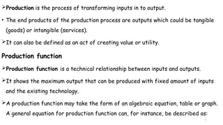
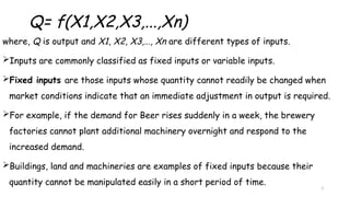
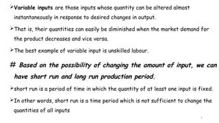
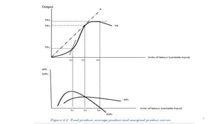
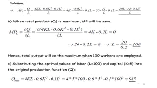
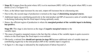
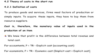
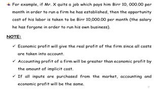
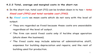
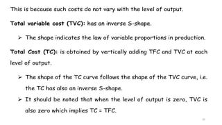
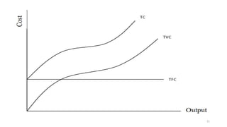
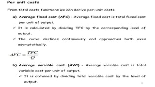
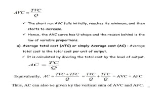
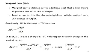
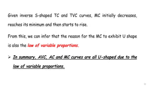
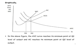
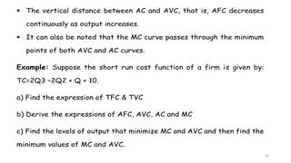
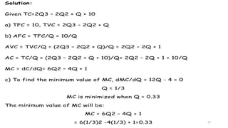
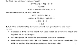
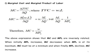
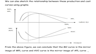
1
Chapter Four
The Theory of Production and Cost
2
Production is the process of transforming inputs in to output.
• The end products of the production process are outputs which could be tangible
(goods) or intangible (services).
It can also be defined as an act of creating value or utility.
Production function
Production function is a technical relationship between inputs and outputs.
It shows the maximum output that can be produced with fixed amount of inputs
and the existing technology.
A production function may take the form of an algebraic equation, table or graph.
A general equation for production function can, for instance, be described as:
3
Q= f(X1,X2,X3,...,Xn)
where, Q is output and X1, X2, X3,…, Xn are different types of inputs.
Inputs are commonly classified as fixed inputs or variable inputs.
Fixed inputs are those inputs whose quantity cannot readily be changed when
market conditions indicate that an immediate adjustment in output is required.
For example, if the demand for Beer rises suddenly in a week, the brewery
factories cannot plant additional machinery overnight and respond to the
increased demand.
Buildings, land and machineries are examples of fixed inputs because their
quantity cannot be manipulated easily in a short period of time.
4
Variable inputs are those inputs whose quantity can be altered almost
instantaneously in response to desired changes in output.
That is, their quantities can easily be diminished when the market demand for
the product decreases and vice versa.
The best example of variable input is unskilled labour.
# Based on the possibility of changing the amount of input, we can
have short run and long run production period.
short run is a period of time in which the quantity of at least one input is fixed.
In other words, short run is a time period which is not sufficient to change the
quantities of all inputs
5
Long run is a period of time in which the quantity of all input is changeable.
• There is sufficient time to change the quantity of all inputs.
• In this section we discuss the short run production period.
Short run production period
• Consider a firm that uses two inputs:
capital (fixed input) and
labour (variable input)
• Since capital is fixed, the firm can increase output only by increasing the amount of
labour it uses. Hence, its production function can be given by:
Q = f (L)
6
• In production, the contribution of a variable input can be described in terms of
total, average and marginal product.
• Total product (TP): it is the total amount of output that can be produced by
efficiently utilizing specific combinations of the variable input and fixed input.
• The TP function in short run follows a certain trend: it initially increases at
increasing rate, increases at decreasing rate, reaches a maximum point and
eventually falls as the quantity of variable input rises.
• Marginal Product (MP): it is the change in output attributed to the addition of
one unit of the variable input to the production process, other inputs being
constant.
• It measures the slope of the total product curve at a given point.
7
• In the short run, the MP of the variable input first increases, reaches its
maximum and then decreases to the extent of being negative.
• That is, as we continue to combine more and more of the variable input with the
fixed input, the MP of the variable input increases initially and then declines.
• Average Product (AP): is the level of output that each unit of input produces, on
the average. Mathematically, it is the ratio of total output to the number of the
variable input.
• AP of labour first increases, reaches its maximum value and eventually declines.
• The AP curve can be measured by the slope of rays originating from the origin to a
point on the TP curve. Consider the following table:
8
9
10
• The relationship between MPL and APL can be stated as follows.
 When APL is increasing, MPL> APL.
 When APL is at its maximum, MPL= APL.
 When APL is decreasing, MPL< APL.
• Example: Suppose the short-run production function of cut-flower firm is:
Q= 4KL -0.6K2 -0.1L2 where Q is quantity of cut-flower produced, L is
labour input and K is fixed capital input (K=5).
a) Determine the average product of labour (APL) function.
b) At what level of labour does the total output of cut-flower reach the maximum?
c) What will be the maximum achievable amount of cut-flower production?
11
b) When total product (Q) is maximum, MP will be zero.
Hence, total output will be the maximum when 100 workers are employed.
c) Substituting the optimal values of labor (L=100) and capital (K=5) into
the original production function (Q):
.
12
The law of variable proportions
It states that as successive units of a variable input (labour) are added to a fixed
input (capital or land), beyond some point, the marginal product that can be
attributed to each additional unit of the variable resource will decline.
This law assumes that technology is fixed and thus the techniques of production
do not change.
Moreover, all units of labour are assumed to be of equal quality.
The law starts to operate after the marginal product curve reaches its maximum
(this happens when the number of workers exceeds L1 in figure 4.1).
This law is also called the law of diminishing returns.
13
Three stages of production
• Stage I: it covers the range of variable input levels over which the average product (APL)
continues to increase.
• It goes from the origin to the point where the APL is maximum, which is the equality of
MPL and APL (up to L2 level of labour employment in figure 4.1).
• This stage is not an efficient region of production though the MP of variable input is
positive.
• The reason is that the variable input (the number of workers) is too small to
efficiently run the fixed input so that the fixed input is under-utilized (not efficiently
utilized).
14
• Stage II: It ranges from the point where APL is at its maximum (MPL=APL) to the point where MPL is zero
(from L2 to L3 in figure 4.1).
• Here, as the labour input increases by one unit, output still increases but at a decreasing rate.
• Due to this, the second stage of production is termed as the stage of diminishing marginal returns.
• Additional inputs are contributing positively to the total product and MP of successive units of variable input
is declining (indicating that the fixed input is being optimally used).
• Hence, the efficient region of production is where the marginal product of the variable input is declining
but positive.
Stage III: This stage is also known as the stage of negative marginal returns to the
variable input.
• The cause of negative marginal returns is the fact that the volume of the variable inputs is quite excessive
relative to the fixed input; the fixed input is over-utilized.
• Obviously, a rational firm should not operate in stage III because additional units of variable input are
contributing negatively to the total product (MP of the variable input is negative).
• In figure 4.1, this stage is indicated by the employment of labour beyond L3.
15
4.2 Theory of costs in the short run
4.2.1 Definition of costs
To produce goods and services, firms need factors of production or
simply inputs. To acquire these inputs, they have to buy them from
resource suppliers.
Cost is, therefore, the monetary value of inputs used in the
production of an item
We know that profit is the difference between total revenue and
total cost.
For accountants, P = TR – Explicit cost (accounting cost)
For economists, P = TR – Economic cost (Implicit cost + Explicit cost)
16
Accounting cost:
Is the monetary value of all purchased inputs used in production.
Are out of pocket expenses for the purchased inputs.
It considers only direct expenses such as wages/salaries, cost of raw
materials, depreciation allowances, interest on borrowed funds and
utility expenses (electricity, water, telephone, etc.).
Economic cost:
Economic cost of producing a commodity considers the monetary value
of all inputs (purchased and non-purchased).
The monetary value of non-purchased inputs is obtained by estimating
their opportunity costs in monetary terms.
The estimated monetary cost for non-purchased inputs is known as
implicit cost.
17
For example, if Mr. X quits a job which pays him Birr 10, 000.00 per
month in order to run a firm he has established, then the opportunity
cost of his labor is taken to be Birr 10,000.00 per month (the salary
he has forgone in order to run his own business).
NOTE:
 Economic profit will give the real profit of the firm since all costs
are taken into account.
 Accounting profit of a firm will be greater than economic profit by
the amount of implicit cost.
 If all inputs are purchased from the market, accounting and
economic profit will be the same.
18
4.2.2 Total, average and marginal costs in the short run
In the short run, total cost (TC) can be broken down in to two – total
fixed cost (TFC) and total variable cost (TVC).
By fixed costs we mean costs which do not vary with the level of
output.
 They are regarded as fixed because these costs are unavoidable
regardless of the level of output.
 The firm can avoid fixed costs only if he/she stops operation
(shuts down the business).
 The fixed costs may include salaries of administrative staff,
expenses for building depreciation and repairs, and the rent of
building used for production.
19
Variable costs, on the other hand, include all costs which directly
vary with the level of output.
 For example, if the firm produces zero output, the variable cost is
zero.
 These costs may include cost of raw materials, the cost of direct
labor and the running expenses of fuel, water, electricity, etc.
In general, the short run total cost is given by the sum of total fixed
cost and total variable cost.
That is, TC = TFC + TVC
Based on the definition of the short run cost functions, let‘s see what
their shapes look like.
Total fixed cost (TFC): is denoted by a straight line parallel to the
output axis.
20
This is because such costs do not vary with the level of output.
Total variable cost (TVC): has an inverse S-shape.
 The shape indicates the law of variable proportions in production.
Total Cost (TC): is obtained by vertically adding TFC and TVC at each
level of output.
 The shape of the TC curve follows the shape of the TVC curve, i.e.
the TC has also an inverse S-shape.
 It should be noted that when the level of output is zero, TVC is
also zero which implies TC = TFC.
21
22
Per unit costs
From total costs functions we can derive per-unit costs.
a) Average fixed cost (AFC) - Average fixed cost is total fixed cost
per unit of output.
 It is calculated by dividing TFC by the corresponding level of
output.
 The curve declines continuously and approaches both axes
asymptotically.
b) Average variable cost (AVC) - Average variable cost is total
variable cost per unit of output.
 It is obtained by dividing total variable cost by the level of
output.
23
 The short run AVC falls initially, reaches its minimum, and then
starts to increase.
 Hence, the AVC curve has U-shape and the reason behind is the
law of variable proportions.
a) Average total cost (ATC) or simply Average cost (AC) - Average
total cost is the total cost per unit of output.
 It is calculated by dividing the total cost by the level of output.
24
Marginal Cost (MC)
o Marginal cost is defined as the additional cost that a firm incurs
to produce one extra unit of output.
o In other words, it is the change in total cost which results from a
unit change in output.
Graphically, MC is the slope of TC function.
In fact, MC is also a change in TVC with respect to a unit change in the
level of output.
25
Given inverse S-shaped TC and TVC curves, MC initially decreases,
reaches its minimum and then starts to rise.
From this, we can infer that the reason for the MC to exhibit U shape
is also the law of variable proportions.
 In summary, AVC, AC and MC curves are all U-shaped due to the
law of variable proportions.
26
Average and marginal cost:
27
Graphically,
 In the above figure, the AVC curve reaches its minimum point at Q1
level of output and AC reaches its minimum point at Q2 level of
output.
28
 The vertical distance between AC and AVC, that is, AFC decreases
continuously as output increases.
 It can also be noted that the MC curve passes through the minimum
points of both AVC and AC curves.
Example: Suppose the short run cost function of a firm is given by:
TC=2Q3 –2Q2 + Q + 10.
a) Find the expression of TFC & TVC
b) Derive the expressions of AFC, AVC, AC and MC
c) Find the levels of output that minimize MC and AVC and then find the
minimum values of MC and AVC.
29
Solution:
Given TC=2Q3 – 2Q2 + Q + 10
a) TFC = 10, TVC = 2Q3 – 2Q2 + Q
b) AFC = TFC/Q = 10/Q
AVC = TVC/Q = (2Q3 – 2Q2 + Q)/Q = 2Q2 – 2Q + 1
AC = TC/Q = (2Q3 – 2Q2 + Q + 10)/Q= 2Q2 – 2Q + 1 + 10/Q
MC = dC/dQ= 6Q2 – 4Q + 1
c) To find the minimum value of MC, dMC/dQ = 12Q - 4 = 0
Q = 1/3
MC is minimized when Q = 0.33
The minimum value of MC will be:
MC = 6Q2 – 4Q + 1
= 6(1/3)2 -4(1/3) + 1=0.33
30
To find the minimum value of AVC
dAVC/dQ = 4Q - 2= 0
Q=0.5
AVC is minimized at Q =0.5
The minimum value of AVC will be:
AVC = 2Q2 – 2Q + 1
AVC = 2 (0.5) 2 - 2(0.5) +1
= 0.5 – 1 + 1
= 0.5
4.2.3 The relationship between short run production and cost
curves
 Suppose a firm in the short run uses labor as a variable input and
capital as a fixed input.
 Let the price of labor be given by w, which is constant.
 Given these conditions, we can derive the relation between MC and
MPL as well as the relation between AVC and APL.
31
i) Marginal Cost and Marginal Product of Labor
The above expression shows that MC and MPL are inversely related.
When initially MPL increases, MC decreases; when MPL is at its
maximum, MC must be at a minimum and when finally MPL declines, MC
increases.
32
ii) Average Variable Cost and Average Product of Labor
This expression also shows inverse relation between AVC and APL. When
APL increases, AVC decreases; when APL is at a maximum, AVC is at a
minimum and when finally APL declines, AVC increases.
33
We can also sketch the relationship between these production and cost
curves using graphs.
From the above figure, we can conclude that the MC curve is the mirror
image of MPL curve and AVC curve is the mirror image of APL curve

chapter four.pptx.ul kyujtrhesdxfghhhhhhhjkkk

  • 1.
    1 Chapter Four The Theoryof Production and Cost
  • 2.
    2 Production is theprocess of transforming inputs in to output. • The end products of the production process are outputs which could be tangible (goods) or intangible (services). It can also be defined as an act of creating value or utility. Production function Production function is a technical relationship between inputs and outputs. It shows the maximum output that can be produced with fixed amount of inputs and the existing technology. A production function may take the form of an algebraic equation, table or graph. A general equation for production function can, for instance, be described as:
  • 3.
    3 Q= f(X1,X2,X3,...,Xn) where, Qis output and X1, X2, X3,…, Xn are different types of inputs. Inputs are commonly classified as fixed inputs or variable inputs. Fixed inputs are those inputs whose quantity cannot readily be changed when market conditions indicate that an immediate adjustment in output is required. For example, if the demand for Beer rises suddenly in a week, the brewery factories cannot plant additional machinery overnight and respond to the increased demand. Buildings, land and machineries are examples of fixed inputs because their quantity cannot be manipulated easily in a short period of time.
  • 4.
    4 Variable inputs arethose inputs whose quantity can be altered almost instantaneously in response to desired changes in output. That is, their quantities can easily be diminished when the market demand for the product decreases and vice versa. The best example of variable input is unskilled labour. # Based on the possibility of changing the amount of input, we can have short run and long run production period. short run is a period of time in which the quantity of at least one input is fixed. In other words, short run is a time period which is not sufficient to change the quantities of all inputs
  • 5.
    5 Long run isa period of time in which the quantity of all input is changeable. • There is sufficient time to change the quantity of all inputs. • In this section we discuss the short run production period. Short run production period • Consider a firm that uses two inputs: capital (fixed input) and labour (variable input) • Since capital is fixed, the firm can increase output only by increasing the amount of labour it uses. Hence, its production function can be given by: Q = f (L)
  • 6.
    6 • In production,the contribution of a variable input can be described in terms of total, average and marginal product. • Total product (TP): it is the total amount of output that can be produced by efficiently utilizing specific combinations of the variable input and fixed input. • The TP function in short run follows a certain trend: it initially increases at increasing rate, increases at decreasing rate, reaches a maximum point and eventually falls as the quantity of variable input rises. • Marginal Product (MP): it is the change in output attributed to the addition of one unit of the variable input to the production process, other inputs being constant. • It measures the slope of the total product curve at a given point.
  • 7.
    7 • In theshort run, the MP of the variable input first increases, reaches its maximum and then decreases to the extent of being negative. • That is, as we continue to combine more and more of the variable input with the fixed input, the MP of the variable input increases initially and then declines. • Average Product (AP): is the level of output that each unit of input produces, on the average. Mathematically, it is the ratio of total output to the number of the variable input. • AP of labour first increases, reaches its maximum value and eventually declines. • The AP curve can be measured by the slope of rays originating from the origin to a point on the TP curve. Consider the following table:
  • 8.
  • 9.
  • 10.
    10 • The relationshipbetween MPL and APL can be stated as follows.  When APL is increasing, MPL> APL.  When APL is at its maximum, MPL= APL.  When APL is decreasing, MPL< APL. • Example: Suppose the short-run production function of cut-flower firm is: Q= 4KL -0.6K2 -0.1L2 where Q is quantity of cut-flower produced, L is labour input and K is fixed capital input (K=5). a) Determine the average product of labour (APL) function. b) At what level of labour does the total output of cut-flower reach the maximum? c) What will be the maximum achievable amount of cut-flower production?
  • 11.
    11 b) When totalproduct (Q) is maximum, MP will be zero. Hence, total output will be the maximum when 100 workers are employed. c) Substituting the optimal values of labor (L=100) and capital (K=5) into the original production function (Q): .
  • 12.
    12 The law ofvariable proportions It states that as successive units of a variable input (labour) are added to a fixed input (capital or land), beyond some point, the marginal product that can be attributed to each additional unit of the variable resource will decline. This law assumes that technology is fixed and thus the techniques of production do not change. Moreover, all units of labour are assumed to be of equal quality. The law starts to operate after the marginal product curve reaches its maximum (this happens when the number of workers exceeds L1 in figure 4.1). This law is also called the law of diminishing returns.
  • 13.
    13 Three stages ofproduction • Stage I: it covers the range of variable input levels over which the average product (APL) continues to increase. • It goes from the origin to the point where the APL is maximum, which is the equality of MPL and APL (up to L2 level of labour employment in figure 4.1). • This stage is not an efficient region of production though the MP of variable input is positive. • The reason is that the variable input (the number of workers) is too small to efficiently run the fixed input so that the fixed input is under-utilized (not efficiently utilized).
  • 14.
    14 • Stage II:It ranges from the point where APL is at its maximum (MPL=APL) to the point where MPL is zero (from L2 to L3 in figure 4.1). • Here, as the labour input increases by one unit, output still increases but at a decreasing rate. • Due to this, the second stage of production is termed as the stage of diminishing marginal returns. • Additional inputs are contributing positively to the total product and MP of successive units of variable input is declining (indicating that the fixed input is being optimally used). • Hence, the efficient region of production is where the marginal product of the variable input is declining but positive. Stage III: This stage is also known as the stage of negative marginal returns to the variable input. • The cause of negative marginal returns is the fact that the volume of the variable inputs is quite excessive relative to the fixed input; the fixed input is over-utilized. • Obviously, a rational firm should not operate in stage III because additional units of variable input are contributing negatively to the total product (MP of the variable input is negative). • In figure 4.1, this stage is indicated by the employment of labour beyond L3.
  • 15.
    15 4.2 Theory ofcosts in the short run 4.2.1 Definition of costs To produce goods and services, firms need factors of production or simply inputs. To acquire these inputs, they have to buy them from resource suppliers. Cost is, therefore, the monetary value of inputs used in the production of an item We know that profit is the difference between total revenue and total cost. For accountants, P = TR – Explicit cost (accounting cost) For economists, P = TR – Economic cost (Implicit cost + Explicit cost)
  • 16.
    16 Accounting cost: Is themonetary value of all purchased inputs used in production. Are out of pocket expenses for the purchased inputs. It considers only direct expenses such as wages/salaries, cost of raw materials, depreciation allowances, interest on borrowed funds and utility expenses (electricity, water, telephone, etc.). Economic cost: Economic cost of producing a commodity considers the monetary value of all inputs (purchased and non-purchased). The monetary value of non-purchased inputs is obtained by estimating their opportunity costs in monetary terms. The estimated monetary cost for non-purchased inputs is known as implicit cost.
  • 17.
    17 For example, ifMr. X quits a job which pays him Birr 10, 000.00 per month in order to run a firm he has established, then the opportunity cost of his labor is taken to be Birr 10,000.00 per month (the salary he has forgone in order to run his own business). NOTE:  Economic profit will give the real profit of the firm since all costs are taken into account.  Accounting profit of a firm will be greater than economic profit by the amount of implicit cost.  If all inputs are purchased from the market, accounting and economic profit will be the same.
  • 18.
    18 4.2.2 Total, averageand marginal costs in the short run In the short run, total cost (TC) can be broken down in to two – total fixed cost (TFC) and total variable cost (TVC). By fixed costs we mean costs which do not vary with the level of output.  They are regarded as fixed because these costs are unavoidable regardless of the level of output.  The firm can avoid fixed costs only if he/she stops operation (shuts down the business).  The fixed costs may include salaries of administrative staff, expenses for building depreciation and repairs, and the rent of building used for production.
  • 19.
    19 Variable costs, onthe other hand, include all costs which directly vary with the level of output.  For example, if the firm produces zero output, the variable cost is zero.  These costs may include cost of raw materials, the cost of direct labor and the running expenses of fuel, water, electricity, etc. In general, the short run total cost is given by the sum of total fixed cost and total variable cost. That is, TC = TFC + TVC Based on the definition of the short run cost functions, let‘s see what their shapes look like. Total fixed cost (TFC): is denoted by a straight line parallel to the output axis.
  • 20.
    20 This is becausesuch costs do not vary with the level of output. Total variable cost (TVC): has an inverse S-shape.  The shape indicates the law of variable proportions in production. Total Cost (TC): is obtained by vertically adding TFC and TVC at each level of output.  The shape of the TC curve follows the shape of the TVC curve, i.e. the TC has also an inverse S-shape.  It should be noted that when the level of output is zero, TVC is also zero which implies TC = TFC.
  • 21.
  • 22.
    22 Per unit costs Fromtotal costs functions we can derive per-unit costs. a) Average fixed cost (AFC) - Average fixed cost is total fixed cost per unit of output.  It is calculated by dividing TFC by the corresponding level of output.  The curve declines continuously and approaches both axes asymptotically. b) Average variable cost (AVC) - Average variable cost is total variable cost per unit of output.  It is obtained by dividing total variable cost by the level of output.
  • 23.
    23  The shortrun AVC falls initially, reaches its minimum, and then starts to increase.  Hence, the AVC curve has U-shape and the reason behind is the law of variable proportions. a) Average total cost (ATC) or simply Average cost (AC) - Average total cost is the total cost per unit of output.  It is calculated by dividing the total cost by the level of output.
  • 24.
    24 Marginal Cost (MC) oMarginal cost is defined as the additional cost that a firm incurs to produce one extra unit of output. o In other words, it is the change in total cost which results from a unit change in output. Graphically, MC is the slope of TC function. In fact, MC is also a change in TVC with respect to a unit change in the level of output.
  • 25.
    25 Given inverse S-shapedTC and TVC curves, MC initially decreases, reaches its minimum and then starts to rise. From this, we can infer that the reason for the MC to exhibit U shape is also the law of variable proportions.  In summary, AVC, AC and MC curves are all U-shaped due to the law of variable proportions.
  • 26.
  • 27.
    27 Graphically,  In theabove figure, the AVC curve reaches its minimum point at Q1 level of output and AC reaches its minimum point at Q2 level of output.
  • 28.
    28  The verticaldistance between AC and AVC, that is, AFC decreases continuously as output increases.  It can also be noted that the MC curve passes through the minimum points of both AVC and AC curves. Example: Suppose the short run cost function of a firm is given by: TC=2Q3 –2Q2 + Q + 10. a) Find the expression of TFC & TVC b) Derive the expressions of AFC, AVC, AC and MC c) Find the levels of output that minimize MC and AVC and then find the minimum values of MC and AVC.
  • 29.
    29 Solution: Given TC=2Q3 –2Q2 + Q + 10 a) TFC = 10, TVC = 2Q3 – 2Q2 + Q b) AFC = TFC/Q = 10/Q AVC = TVC/Q = (2Q3 – 2Q2 + Q)/Q = 2Q2 – 2Q + 1 AC = TC/Q = (2Q3 – 2Q2 + Q + 10)/Q= 2Q2 – 2Q + 1 + 10/Q MC = dC/dQ= 6Q2 – 4Q + 1 c) To find the minimum value of MC, dMC/dQ = 12Q - 4 = 0 Q = 1/3 MC is minimized when Q = 0.33 The minimum value of MC will be: MC = 6Q2 – 4Q + 1 = 6(1/3)2 -4(1/3) + 1=0.33
  • 30.
    30 To find theminimum value of AVC dAVC/dQ = 4Q - 2= 0 Q=0.5 AVC is minimized at Q =0.5 The minimum value of AVC will be: AVC = 2Q2 – 2Q + 1 AVC = 2 (0.5) 2 - 2(0.5) +1 = 0.5 – 1 + 1 = 0.5 4.2.3 The relationship between short run production and cost curves  Suppose a firm in the short run uses labor as a variable input and capital as a fixed input.  Let the price of labor be given by w, which is constant.  Given these conditions, we can derive the relation between MC and MPL as well as the relation between AVC and APL.
  • 31.
    31 i) Marginal Costand Marginal Product of Labor The above expression shows that MC and MPL are inversely related. When initially MPL increases, MC decreases; when MPL is at its maximum, MC must be at a minimum and when finally MPL declines, MC increases.
  • 32.
    32 ii) Average VariableCost and Average Product of Labor This expression also shows inverse relation between AVC and APL. When APL increases, AVC decreases; when APL is at a maximum, AVC is at a minimum and when finally APL declines, AVC increases.
  • 33.
    33 We can alsosketch the relationship between these production and cost curves using graphs. From the above figure, we can conclude that the MC curve is the mirror image of MPL curve and AVC curve is the mirror image of APL curve