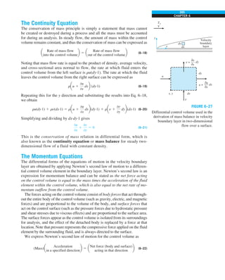
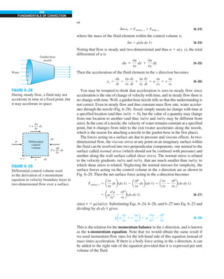
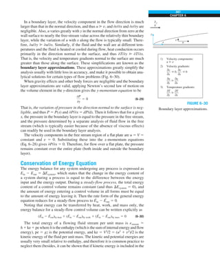
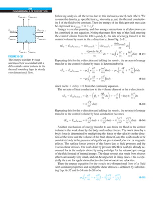
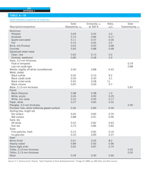
This document contains quotes related to ethics from notable figures such as Jacques Cousteau, Laura Schlessinger, Manly Hall, Albert Einstein, Martin Luther King Jr., Theodore Roosevelt, Said Nursi, and Ralph Walser Emerson. It also contains information about the textbook "Heat and Mass Transfer: Fundamentals & Applications" including the authors Yunus A. Çengel and Afshin J. Ghajar, as well as a brief description of the chapters included in the textbook.


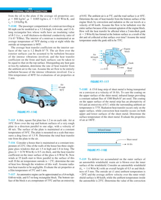
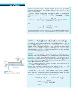
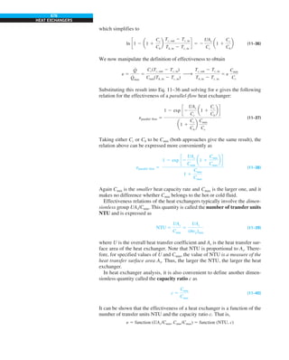
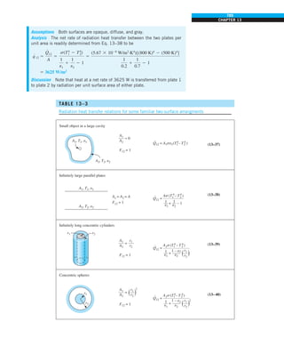
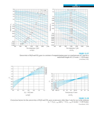
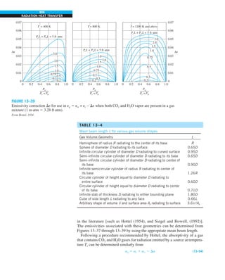
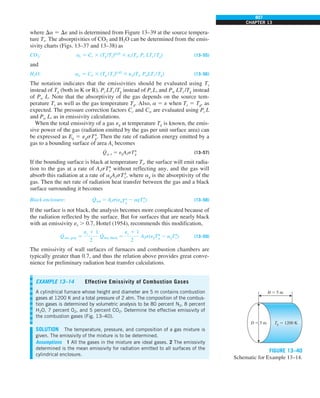
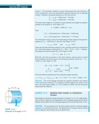
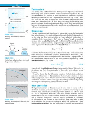
![25
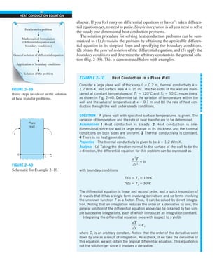
CHAPTER 1
1–7 ■
CONVECTION
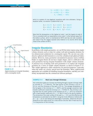
Convection is the mode of energy transfer between a solid surface and the
adjacent liquid or gas that is in motion, and it involves the combined effects
of conduction and fluid motion. The faster the fluid motion, the greater the
convection heat transfer. In the absence of any bulk fluid motion, heat trans-
fer between a solid surface and the adjacent fluid is by pure conduction. The
presence of bulk motion of the fluid enhances the heat transfer between the
solid surface and the fluid, but it also complicates the determination of heat
transfer rates.
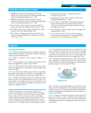
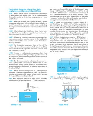
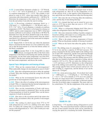
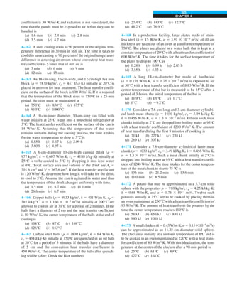
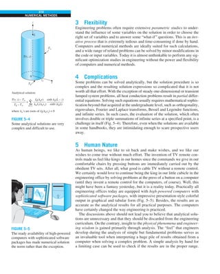
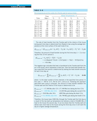
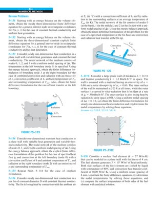
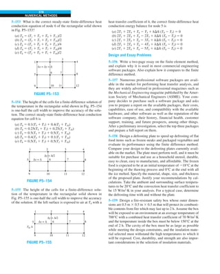
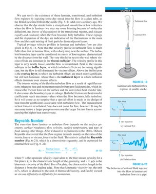
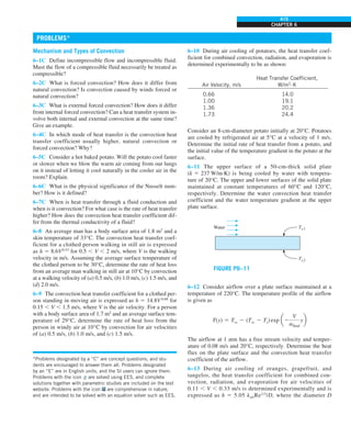
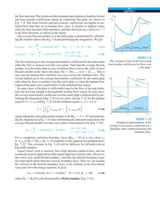
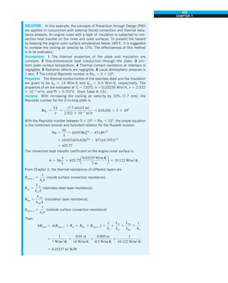
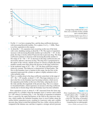
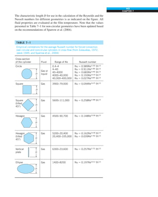
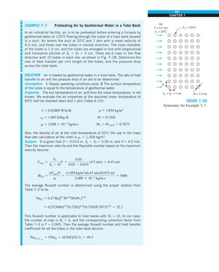
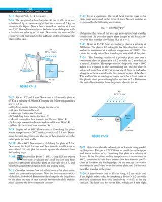
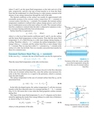
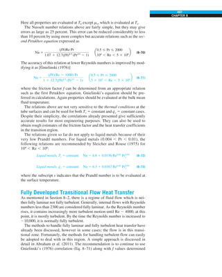
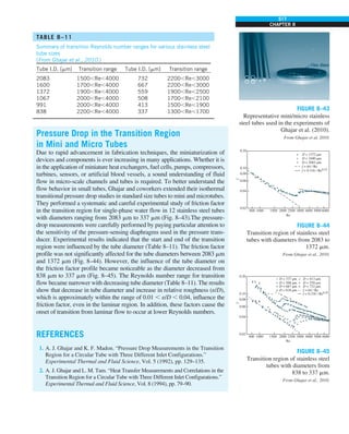
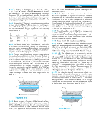
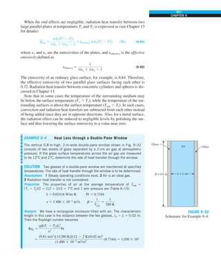
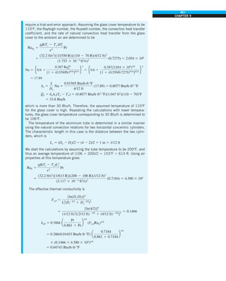
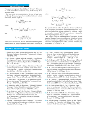
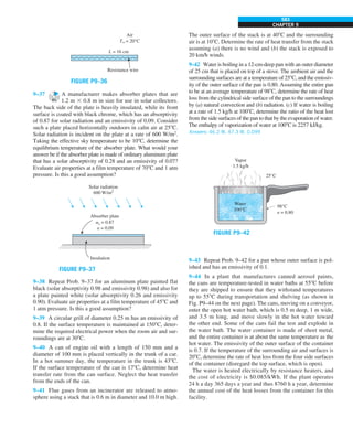
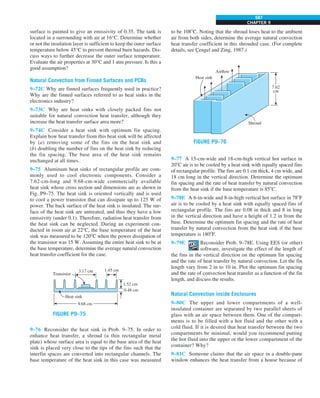
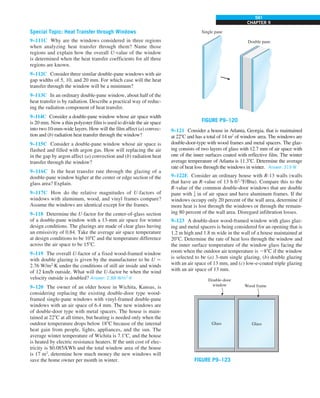
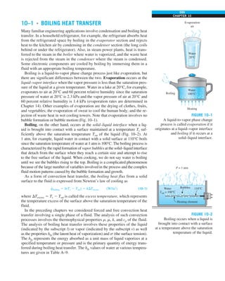
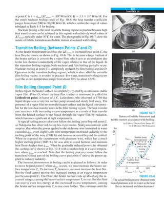
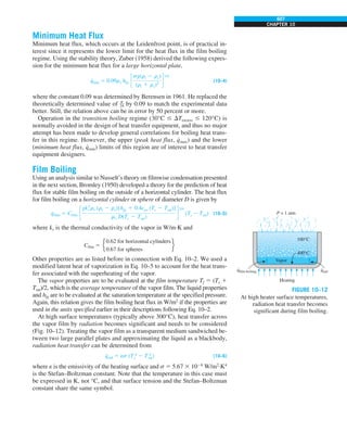
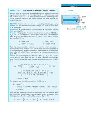
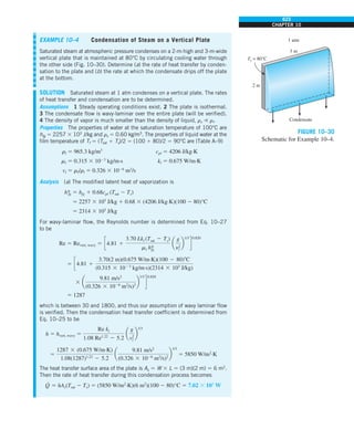
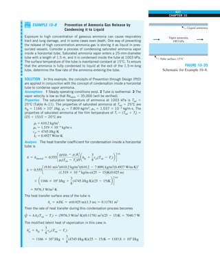
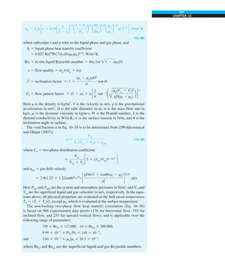
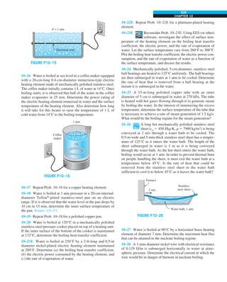
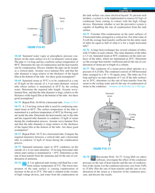
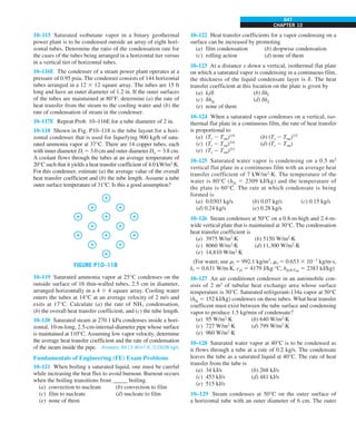
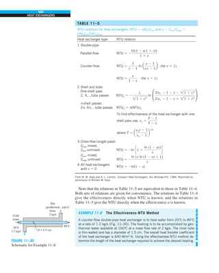
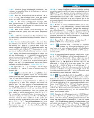
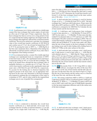
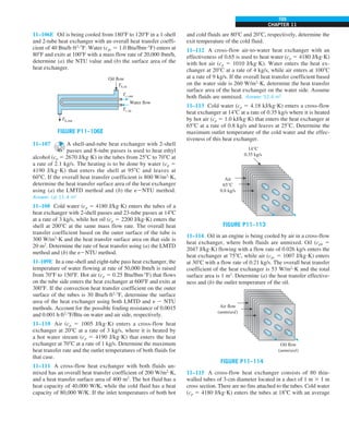
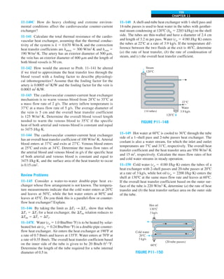
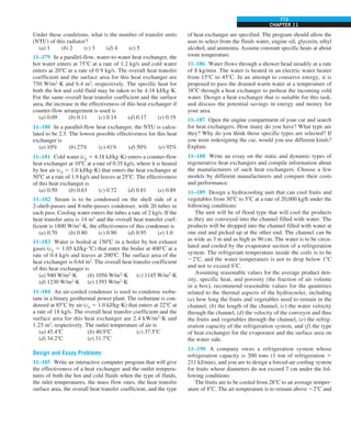
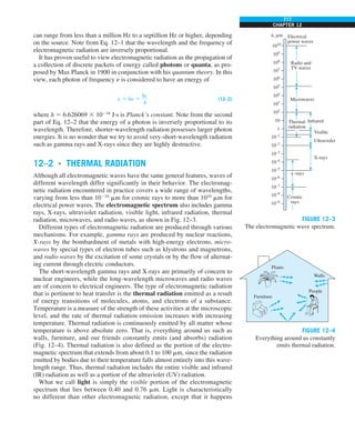
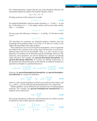
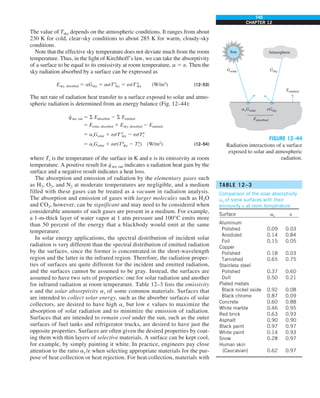
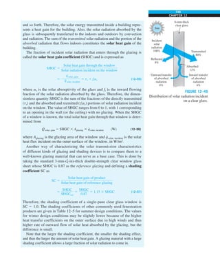
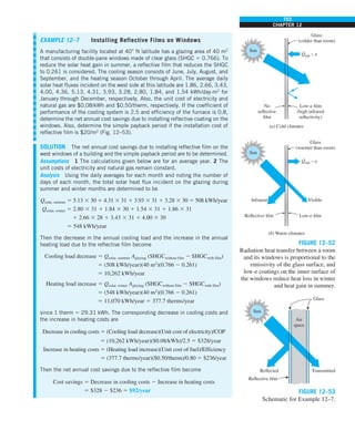
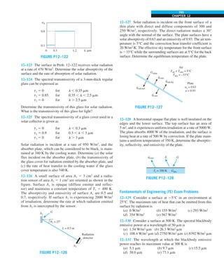
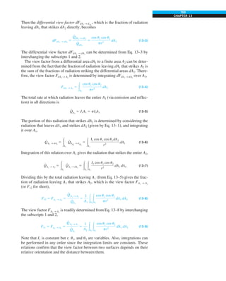
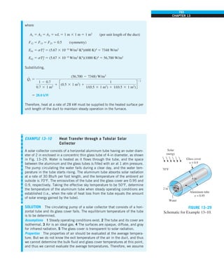
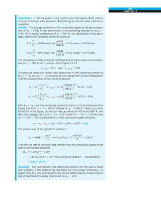
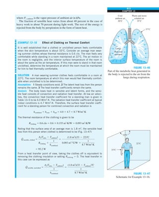
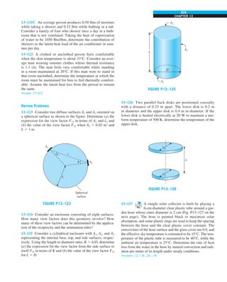
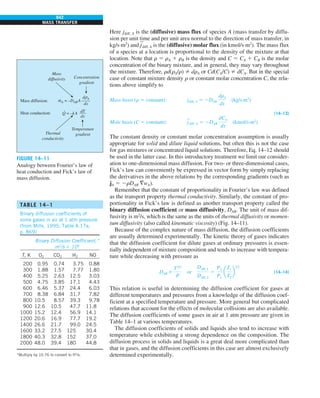
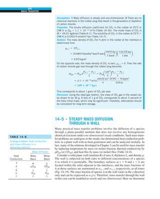
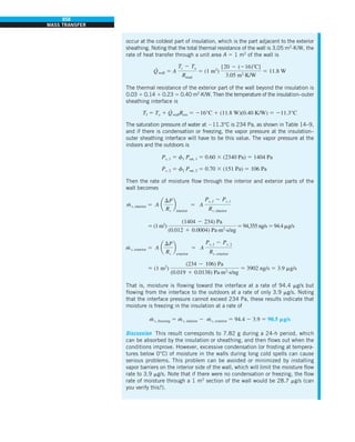
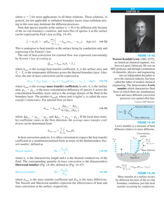
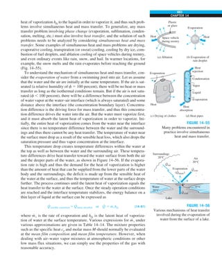
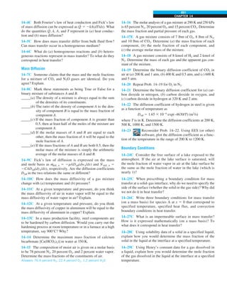
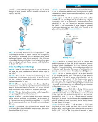
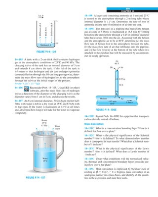
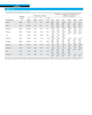
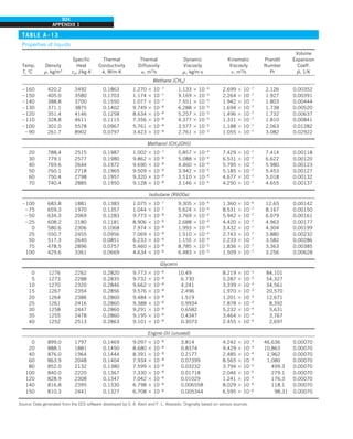
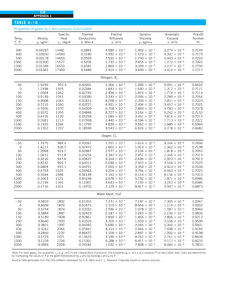
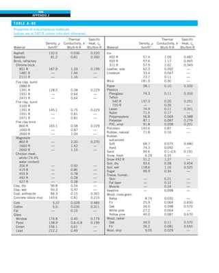
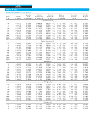
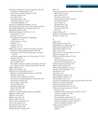
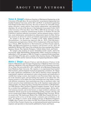
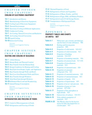
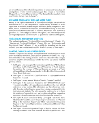
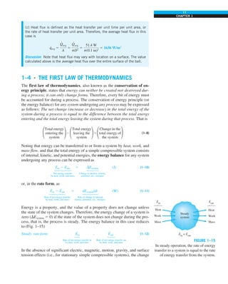
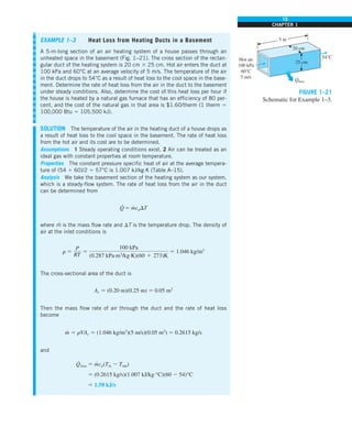
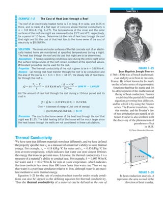
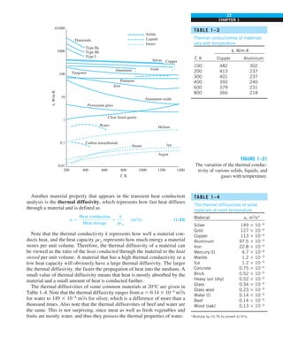
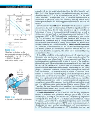
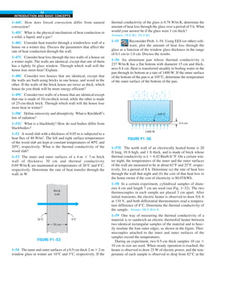
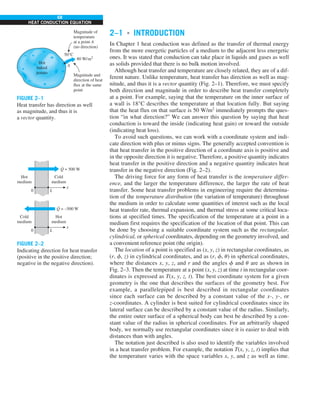
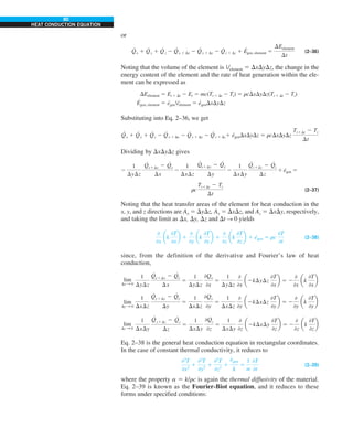
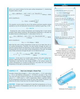
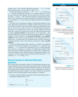
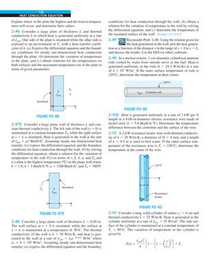
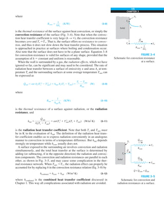
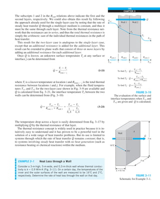
EXAMPLE 1–7 Conversion between SI and English Units
An engineer who is working on the heat transfer analysis of a brick building in
English units needs the thermal conductivity of brick. But the only value he
can find from his handbooks is 0.72 W/m·°C, which is in SI units. To make
matters worse, the engineer does not have a direct conversion factor between
the two unit systems for thermal conductivity. Can you help him out?
SOLUTION The situation this engineer is facing is not unique, and most engi-
neers often find themselves in a similar position. A person must be very care-
ful during unit conversion not to fall into some common pitfalls and to avoid
some costly mistakes. Although unit conversion is a simple process, it requires
utmost care and careful reasoning.
The conversion factors for W and m are straightforward and are given in con-
version tables to be
1 W 5 3.41214 Btu/h
1 m 5 3.2808 ft
But the conversion of °C into °F is not so simple, and it can be a source of
error if one is not careful. Perhaps the first thought that comes to mind is to
replace °C by (°F 2 32)/1.8 since T(°C) 5 [T(°F) 2 32]/1.8. But this will be
wrong since the °C in the unit W/m·°C represents per °C change in tempera-
ture. Noting that 1°C change in temperature corresponds to 1.8°F, the proper
conversion factor to be used is
1°C 5 1.8°F
Substituting, we get
1 W/m·°C 5
3.41214 Btu/h
(3.2808 ft)(1.88F)
5 0.5778 Btu/h·ft·°F
which is the desired conversion factor. Therefore, the thermal conductivity of
the brick in English units is
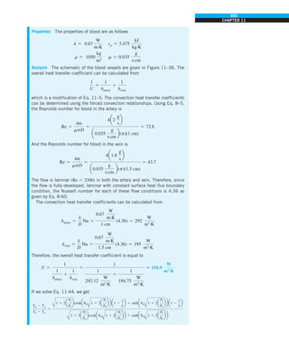
kbrick 5 0.72 W/m·°C
5 0.72 3 (0.5778 Btu/h·ft·°F)
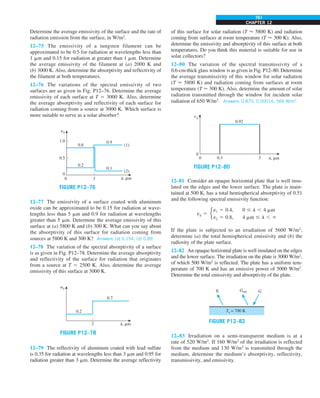
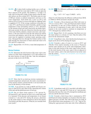
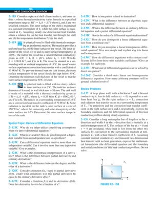
5 0.42 Btu/h·ft·°F
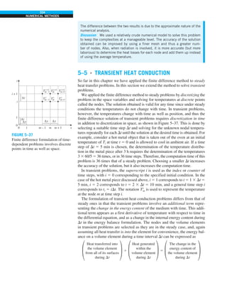
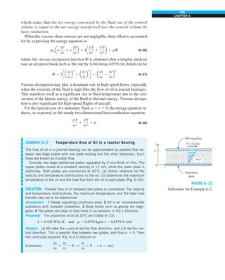
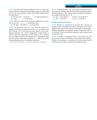
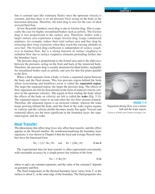
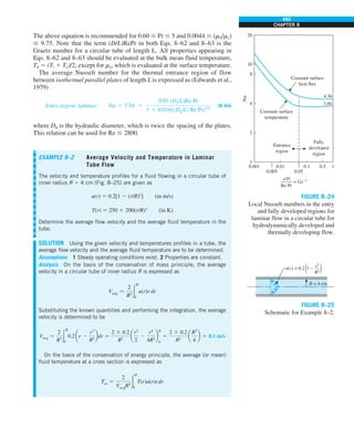
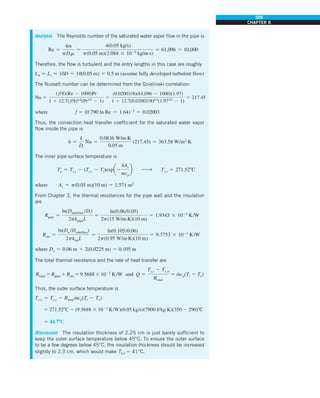
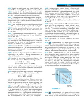
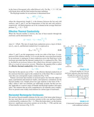
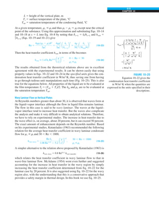
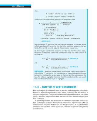
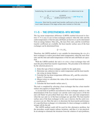
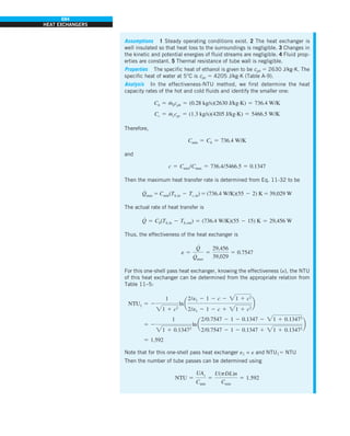
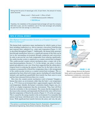
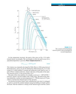
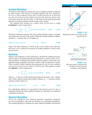
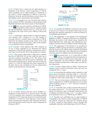
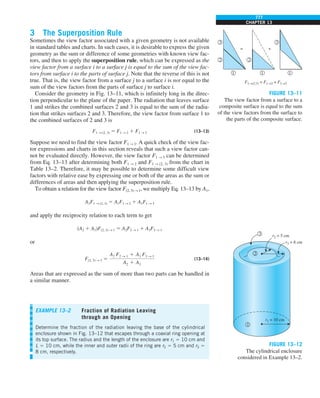
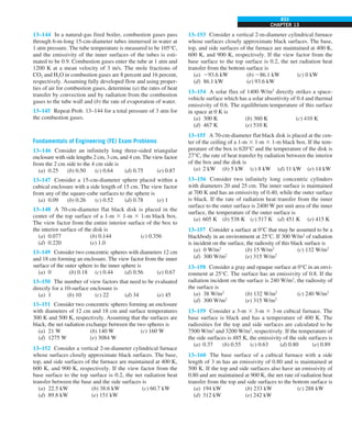
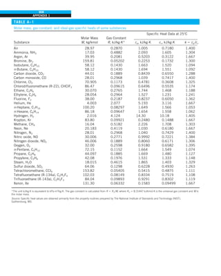
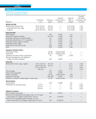
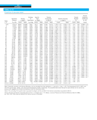
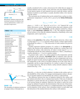
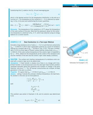
Discussion Note that the thermal conductivity value of a material in English
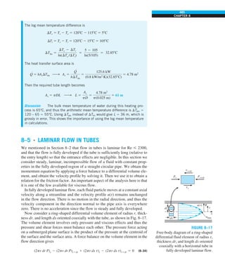
units is about half that in SI units (Fig. 1–33). Also note that we rounded
the result to two significant digits (the same number in the original value)
since expressing the result in more significant digits (such as 0.4160 instead
of 0.42) would falsely imply a more accurate value than the original one.
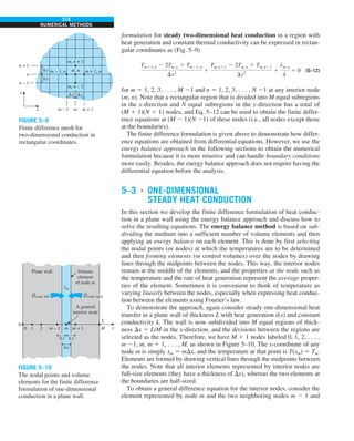
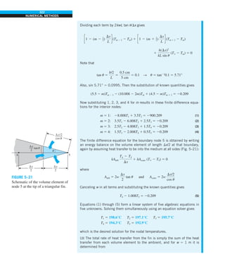
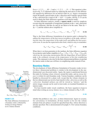
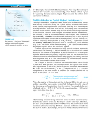
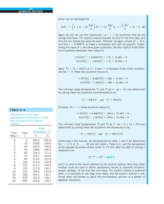
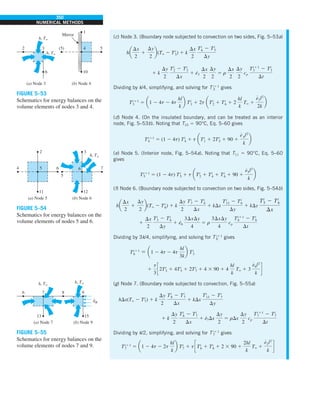
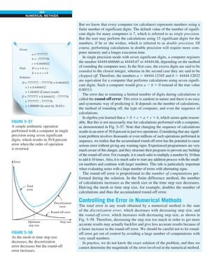
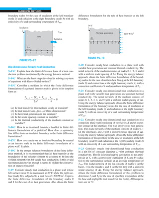
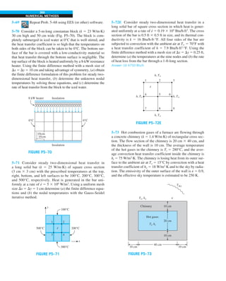
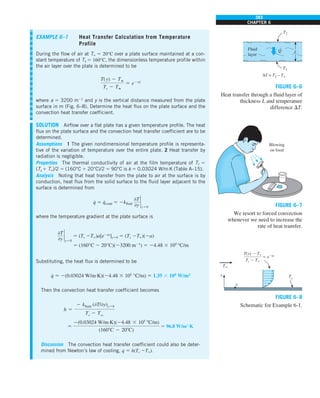
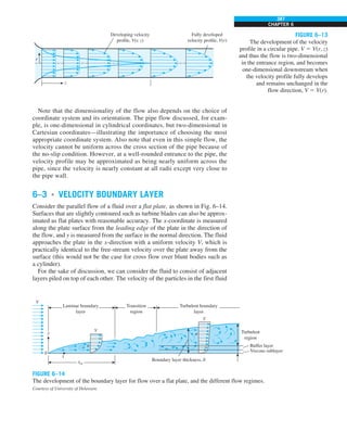
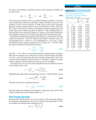
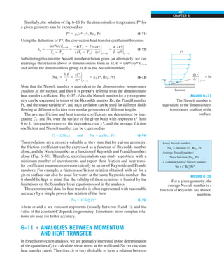
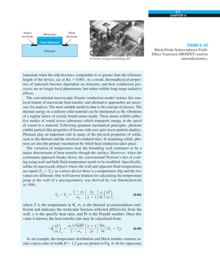
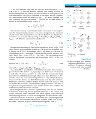
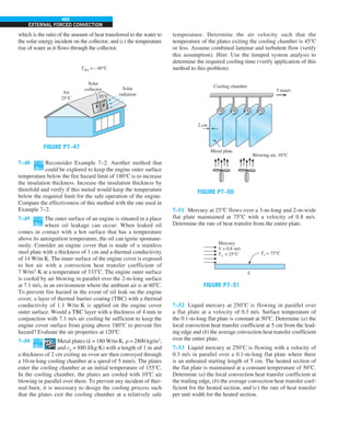
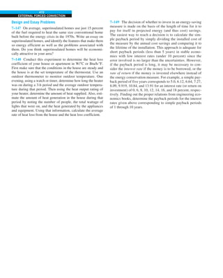
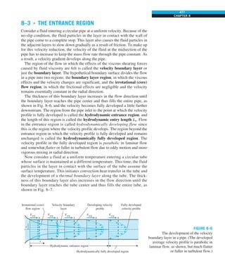
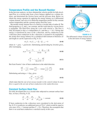
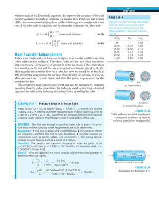
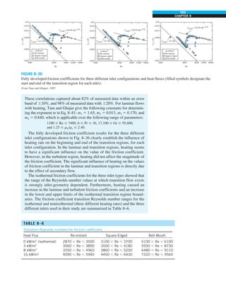
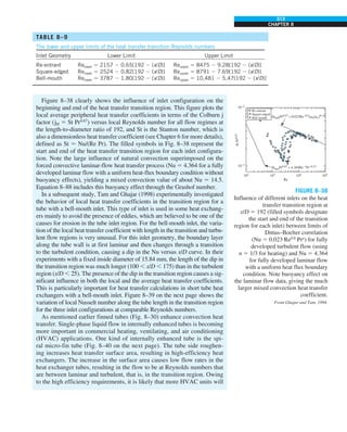
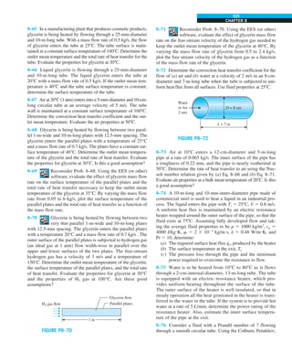
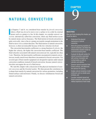
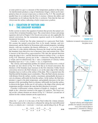
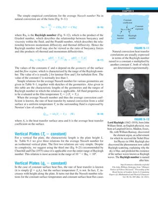
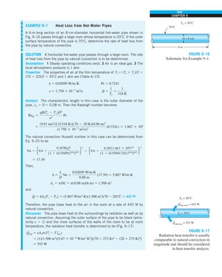
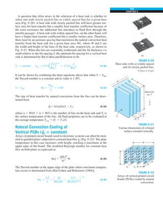
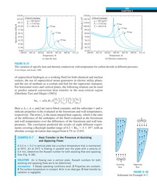
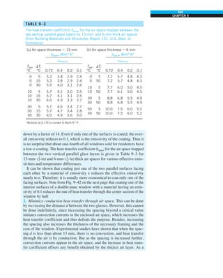
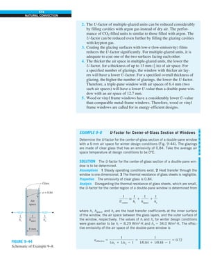
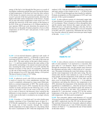
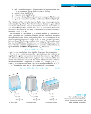
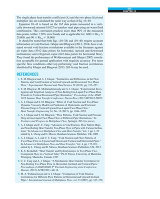
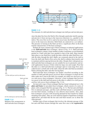
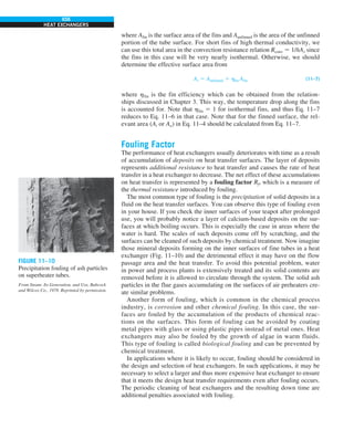
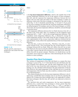
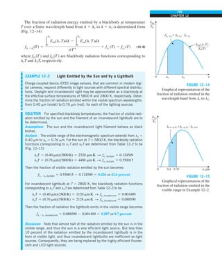
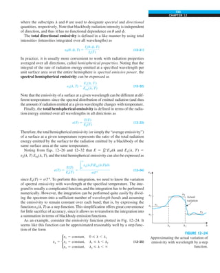
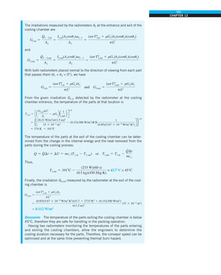
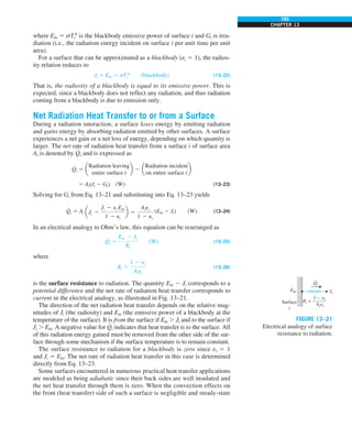
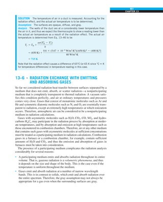
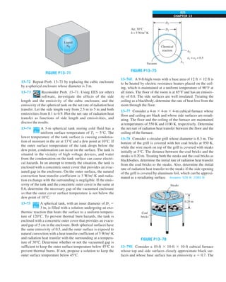
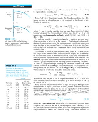
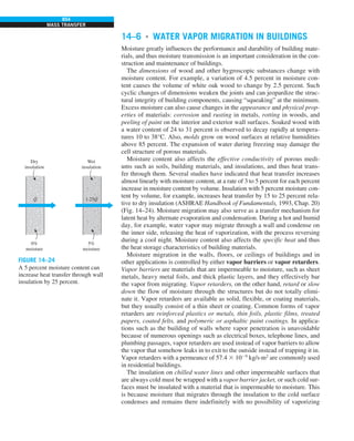
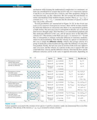
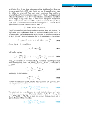
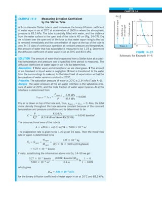
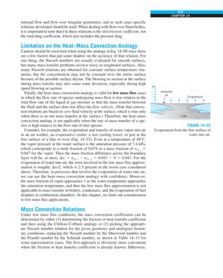
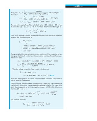
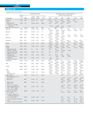
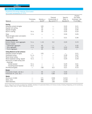
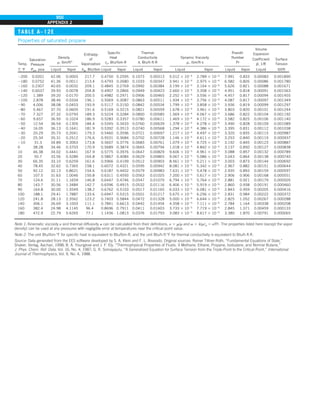
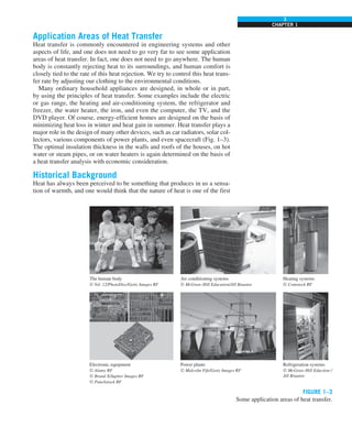
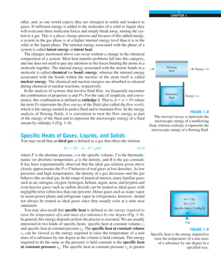
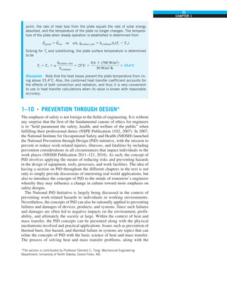
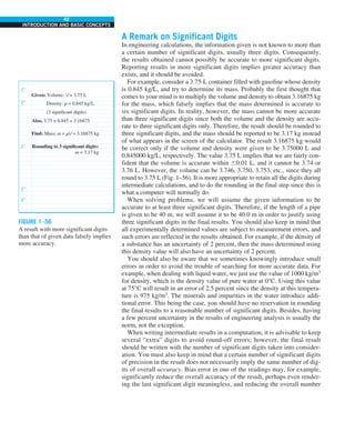
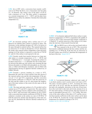
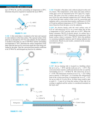
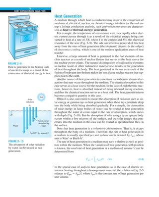
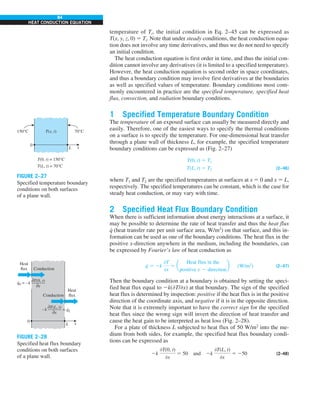
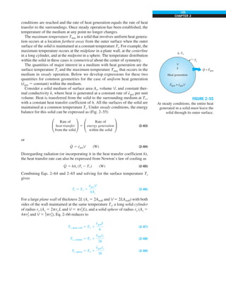
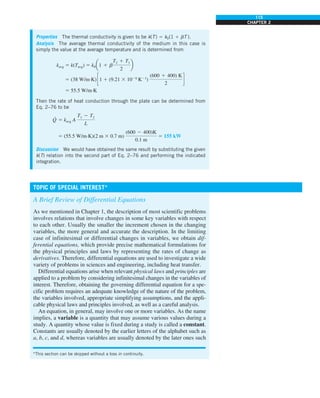
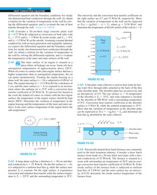
FIGURE 1–33
The thermal conductivity value in
English units is obtained by multiplying
the value in SI units by 0.5778.
= 0.42 Btu/h·ft·°F
k = 0.72 W/m·°C](https://image.slidesharecdn.com/25489135-230110133727-3d40a16a/85/25489135-pdf-48-320.jpg)
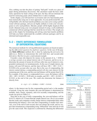
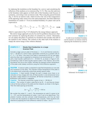
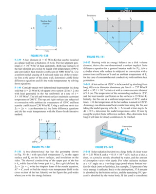
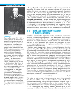
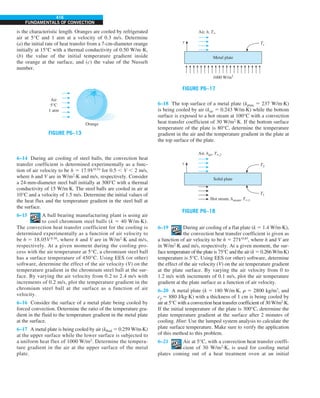
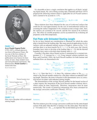
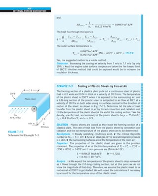
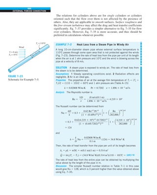
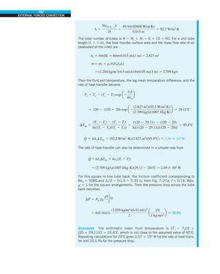
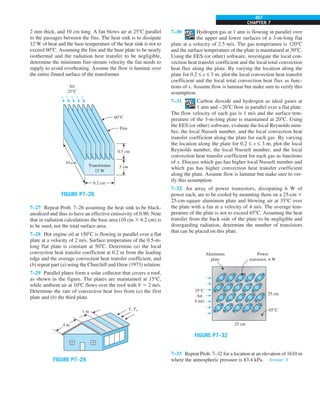
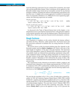
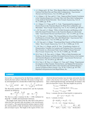
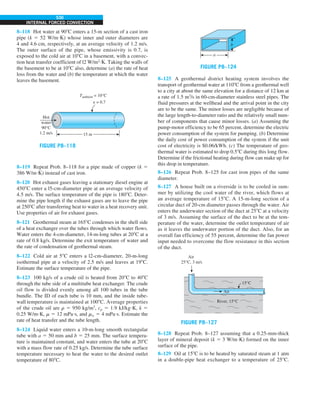
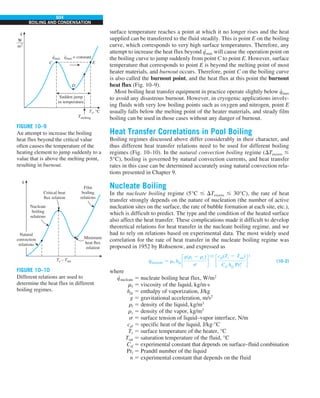
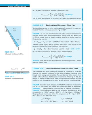
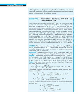
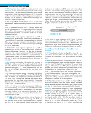
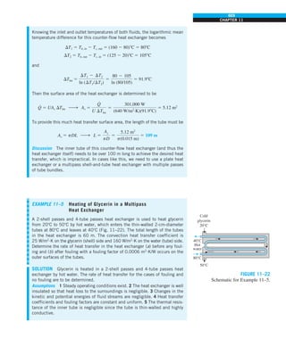
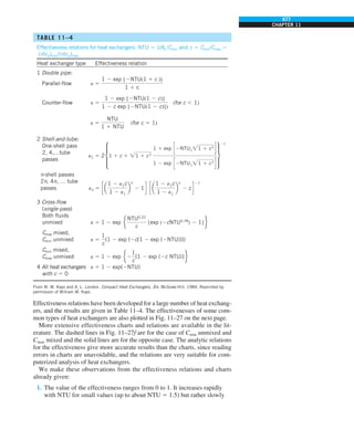
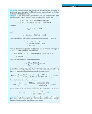
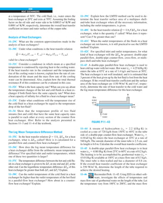
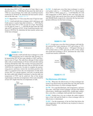
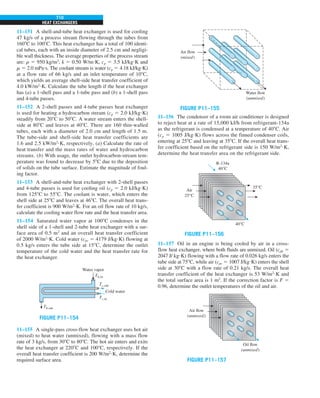
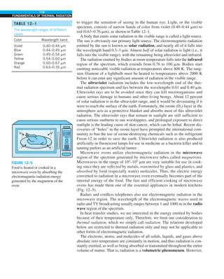
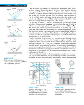
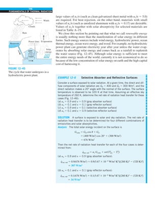
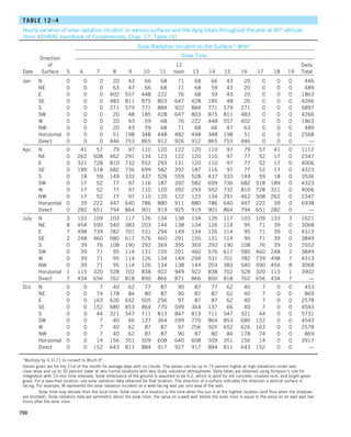
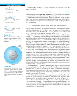
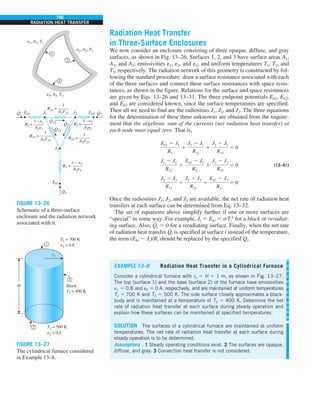
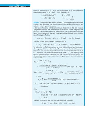
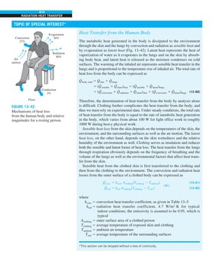
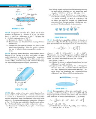
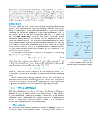
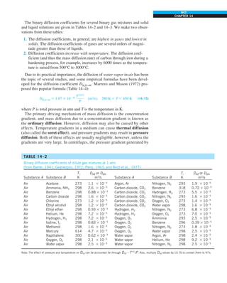
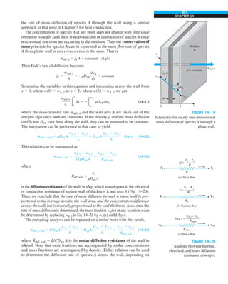
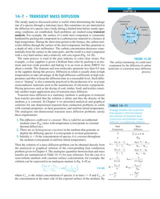
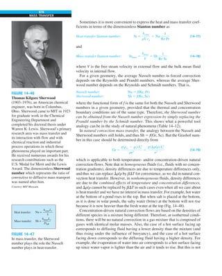
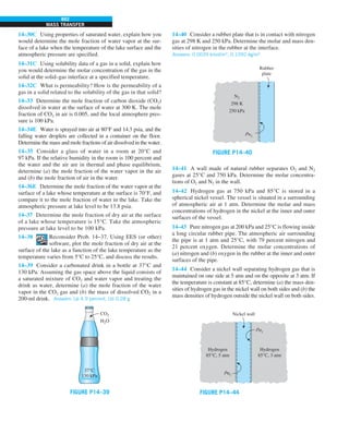
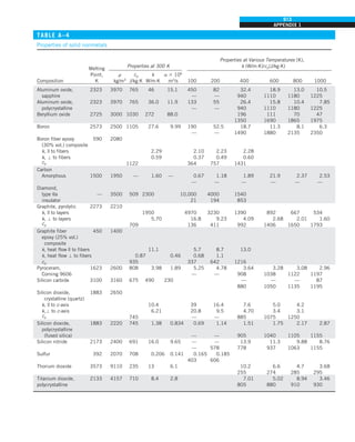
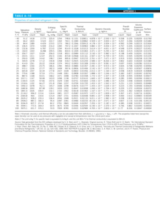
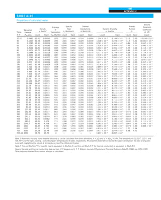
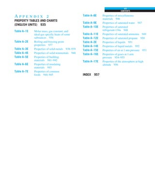
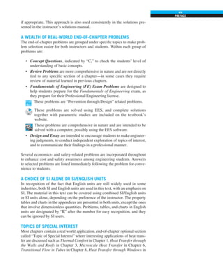
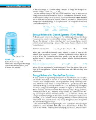
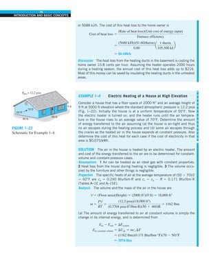
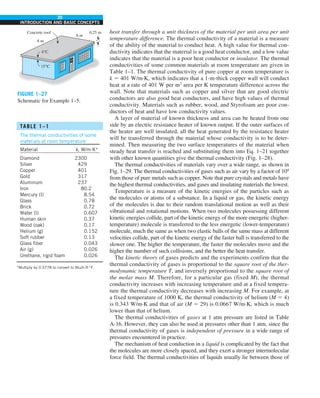
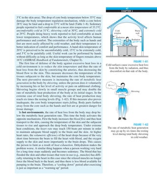
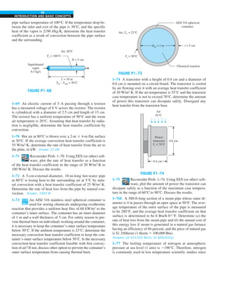
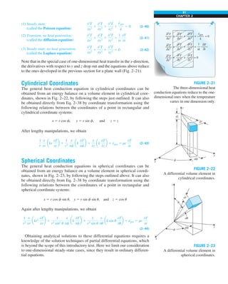
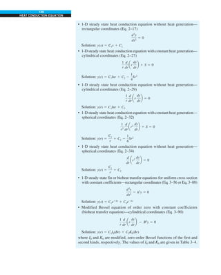
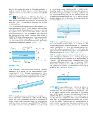
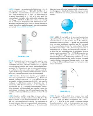
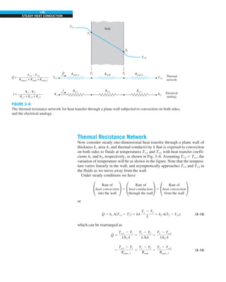
![30
INTRODUCTION AND BASIC CONCEPTS
1–9 ■
SIMULTANEOUS HEAT TRANSFER
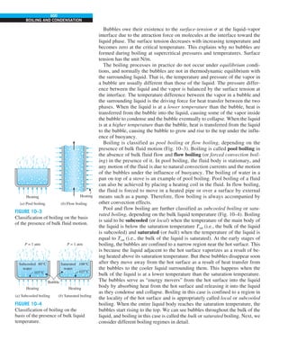
MECHANISMS
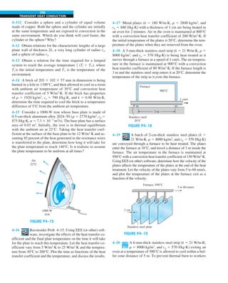
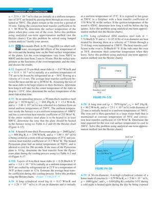
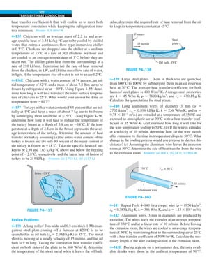
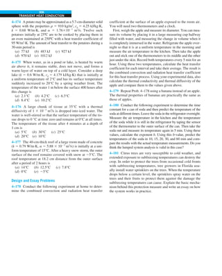
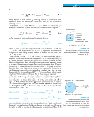
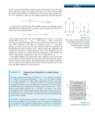
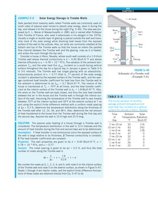
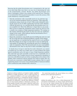
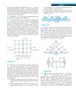
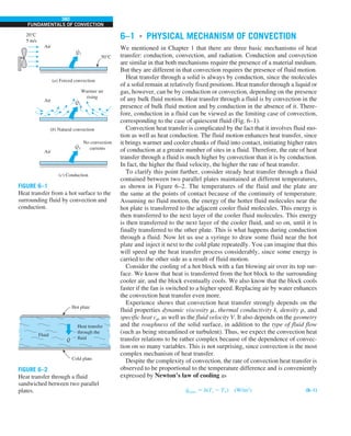
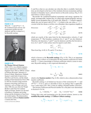
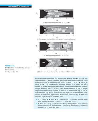
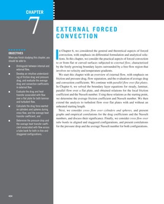
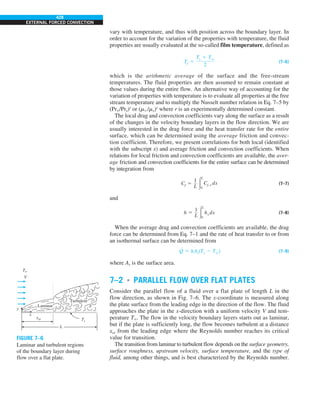
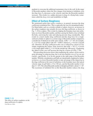
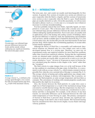
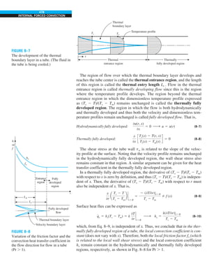
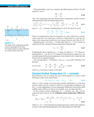
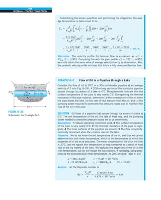
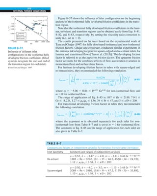
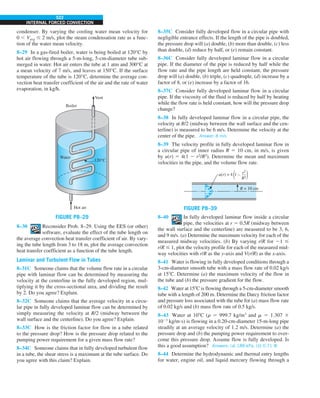
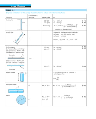
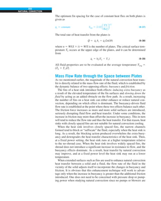
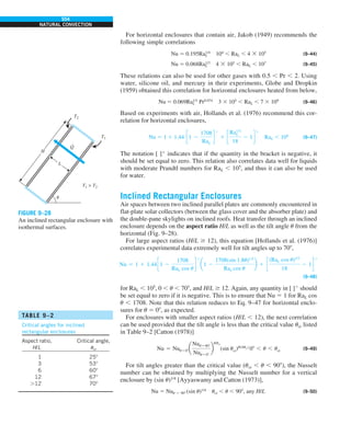
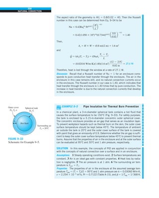
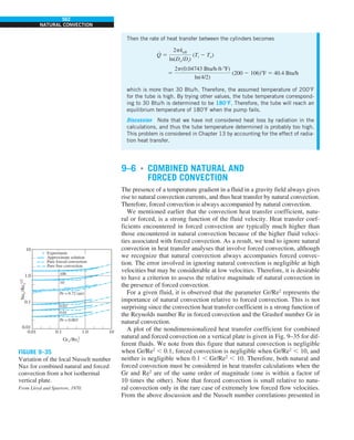
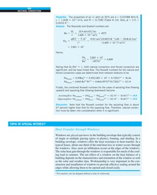
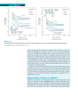
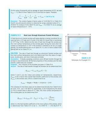
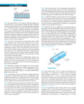
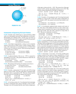
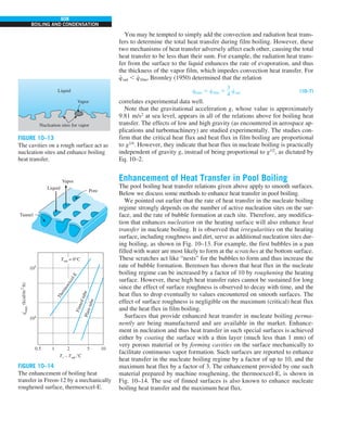
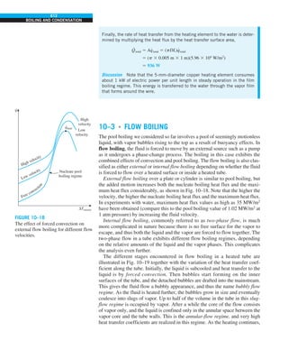
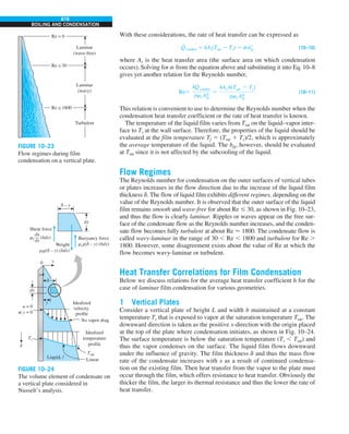
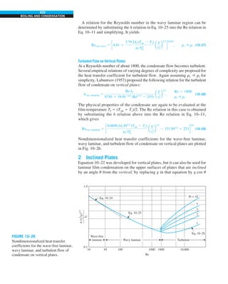
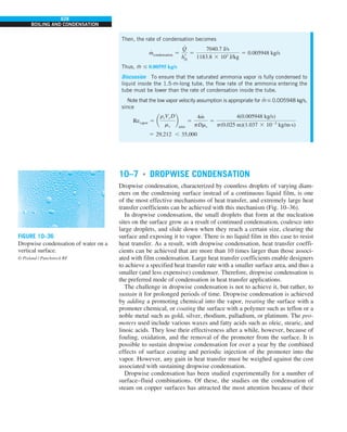
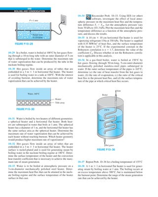
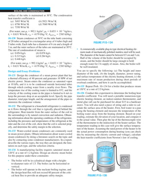
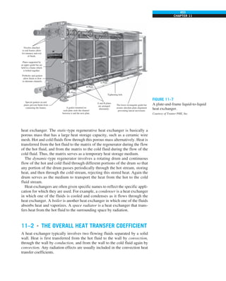
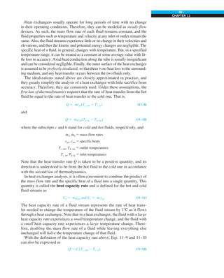
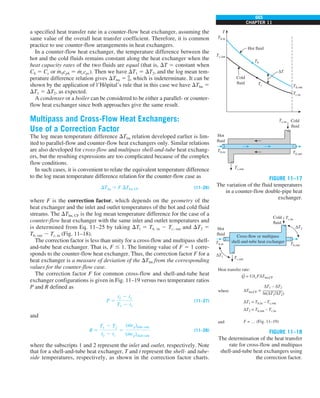
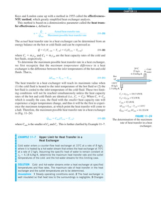
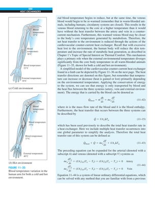
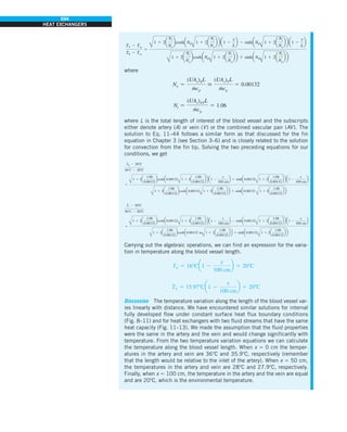
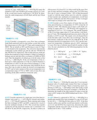
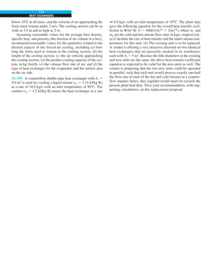
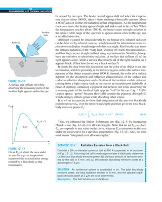
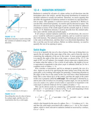
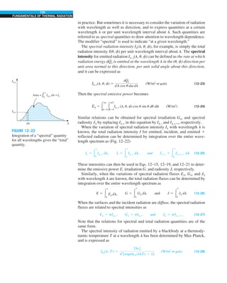
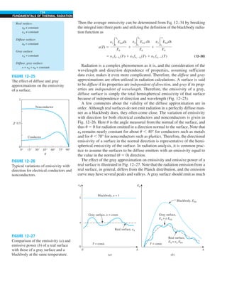
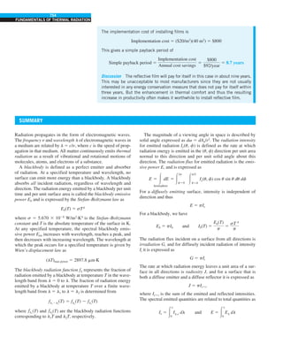
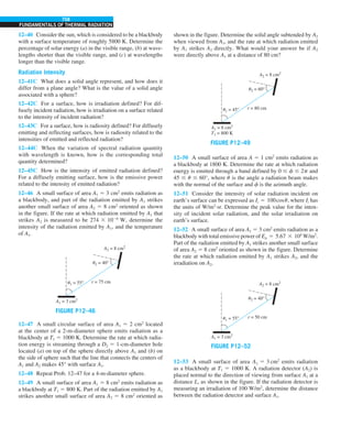
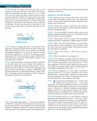
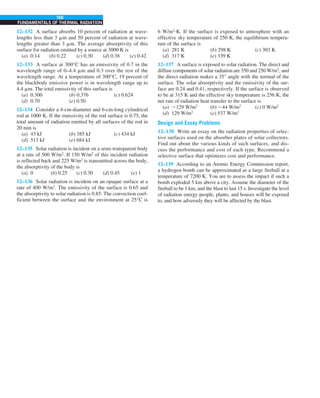
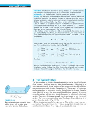
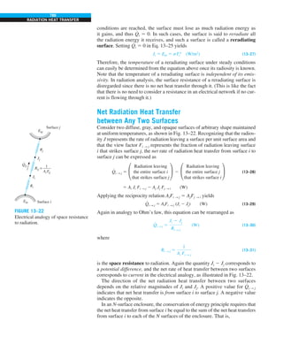
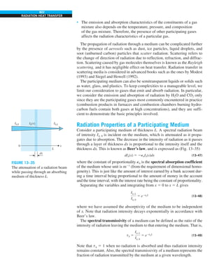
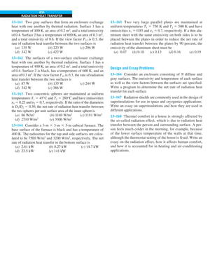
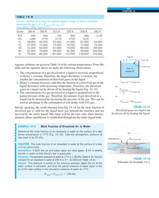
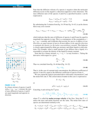
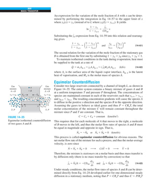
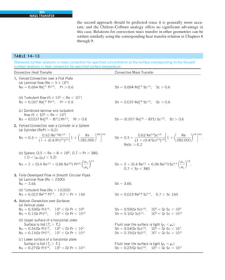
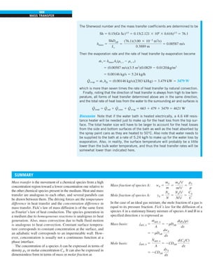
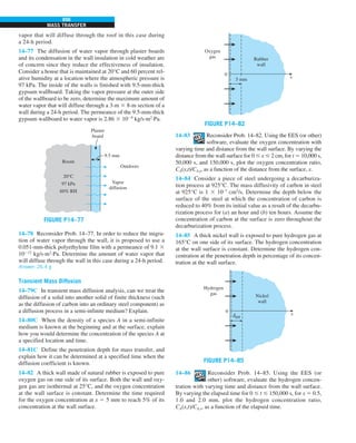
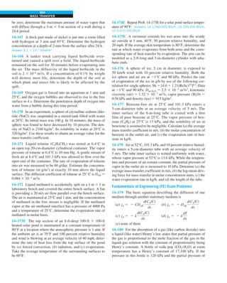
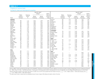
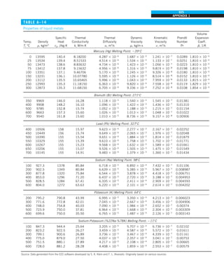
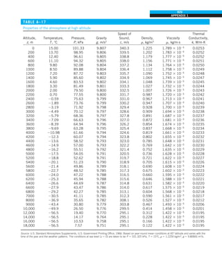
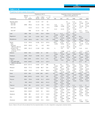
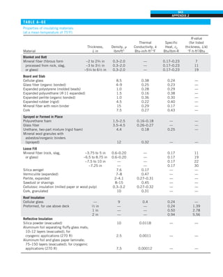
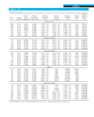
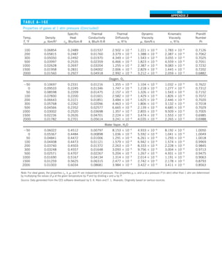
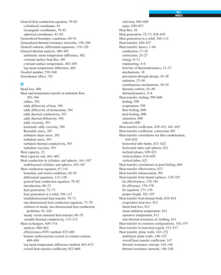
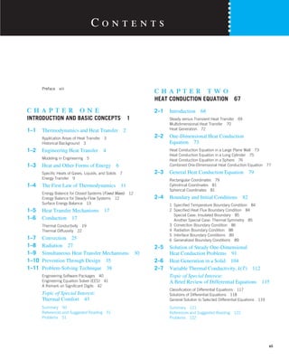
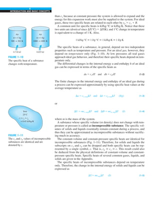
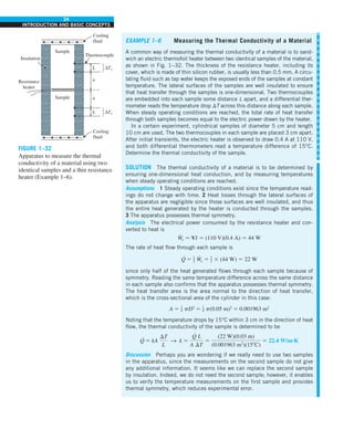
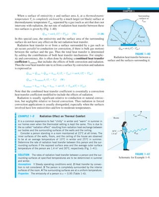
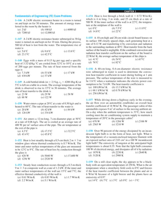
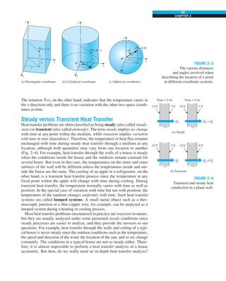
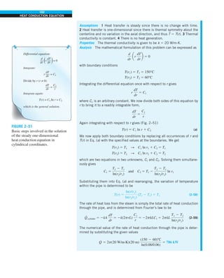
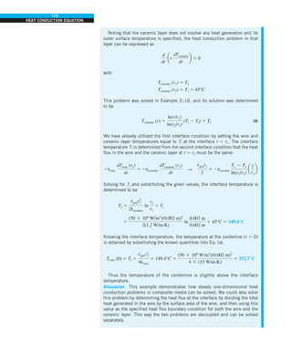
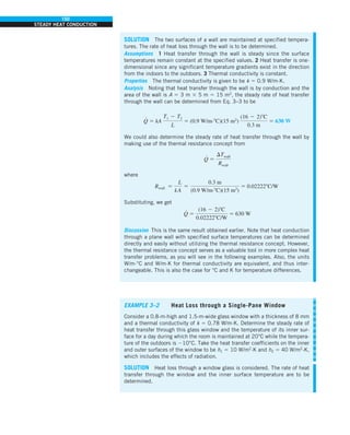
We mentioned that there are three mechanisms of heat transfer, but not all
three can exist simultaneously in a medium. For example, heat transfer is only
by conduction in opaque solids, but by conduction and radiation in semitrans-
parent solids. Thus, a solid may involve conduction and radiation but not
convection. However, a solid may involve heat transfer by convection and/or
radiation on its surfaces exposed to a fluid or other surfaces. For example, the
outer surfaces of a cold piece of rock will warm up in a warmer environment
as a result of heat gain by convection (from the air) and radiation (from the sun
or the warmer surrounding surfaces). But the inner parts of the rock will warm
up as this heat is transferred to the inner region of the rock by conduction.
Heat transfer is by conduction and possibly by radiation in a still fluid (no
bulk fluid motion) and by convection and radiation in a flowing fluid. In the
absence of radiation, heat transfer through a fluid is either by conduction or
convection, depending on the presence of any bulk fluid motion. Convection
can be viewed as combined conduction and fluid motion, and conduction in a
fluid can be viewed as a special case of convection in the absence of any fluid
motion (Fig. 1–42).
Thus, when we deal with heat transfer through a fluid, we have either con-
duction or convection, but not both. Also, gases are practically transparent to
radiation, except that some gases are known to absorb radiation strongly at
certain wavelengths. Ozone, for example, strongly absorbs ultraviolet radia-
tion. But in most cases, a gas between two solid surfaces does not interfere
with radiation and acts effectively as a vacuum. Liquids, on the other hand,
are usually strong absorbers of radiation.
Finally, heat transfer through a vacuum is by radiation only since conduc-
tion or convection requires the presence of a material medium.
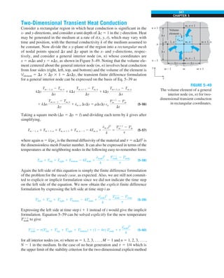
Analysis The net rates of radiation heat transfer from the body to the sur-
rounding walls, ceiling, and floor in winter and summer are
Q
·
rad, winter 5 esAs (T 4
s 2 T 4
surr, winter)
5 (0.95)(5.67 3 1028
W/m2
·K4
)(1.4 m2
)
3 [(30 1 273)4
2 (10 1 273)4
] K4
5 152 W
and
Q
·
rad, summer 5 esAs (T 4
s 2 T 4
surr, summer)
5 (0.95)(5.67 3 1028
W/m2
·K4
)(1.4 m2
)
3 [(30 1 273)4
2 (25 1 273)4
] K4
5 40.9 W
Discussion Note that we must use thermodynamic (i.e., absolute) temperatures
in radiation calculations. Also note that the rate of heat loss from the person by
radiation is almost four times as large in winter than it is in summer, which explains
the “chill” we feel in winter even if the thermostat setting is kept the same.
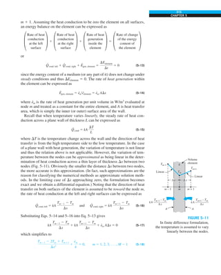
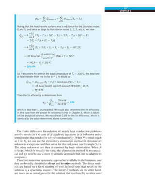
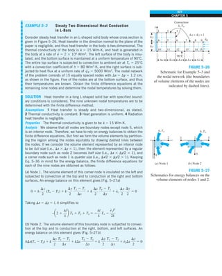
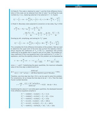
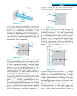
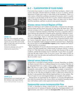
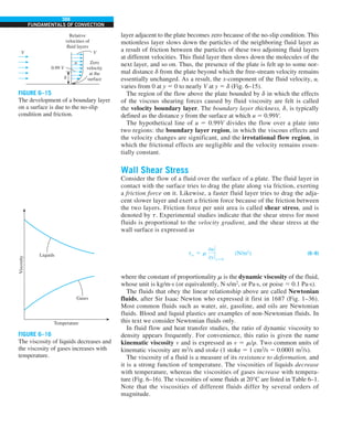
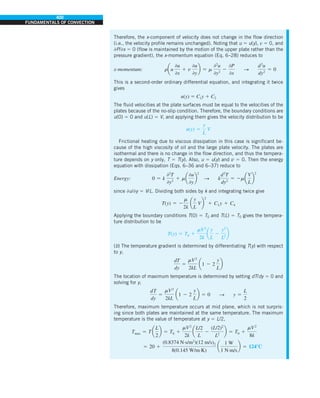
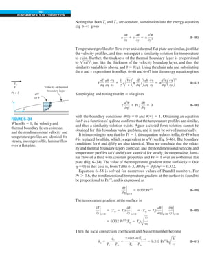
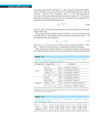
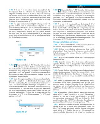
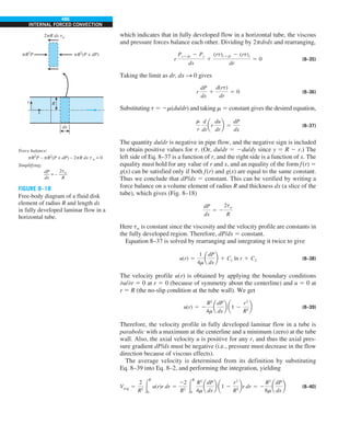
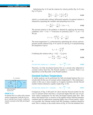
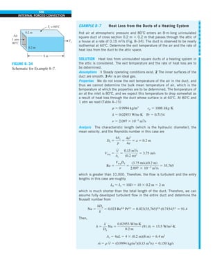
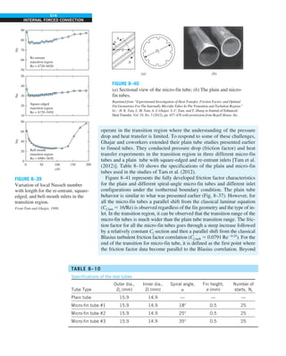
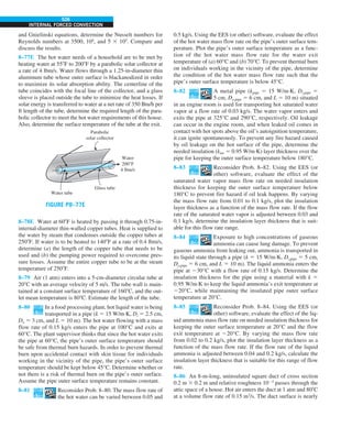
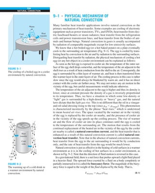
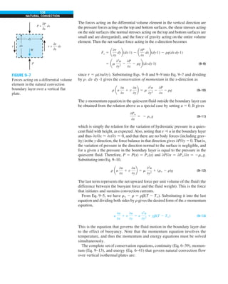
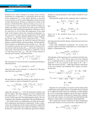
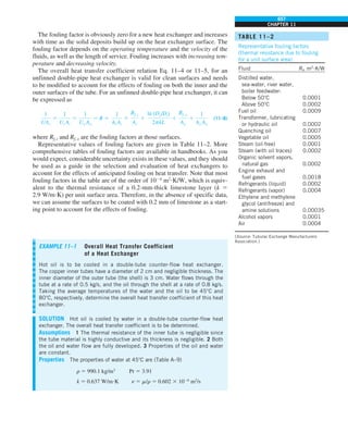
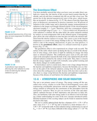
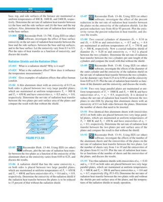
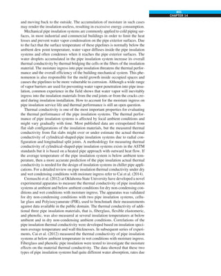
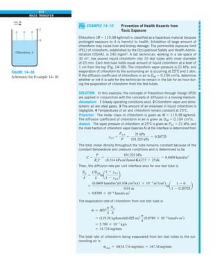
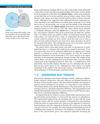
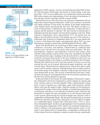
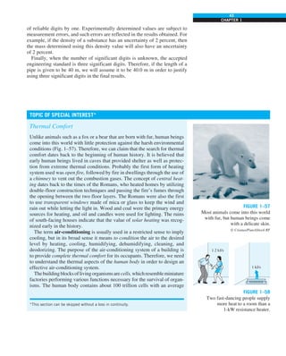
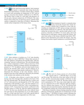
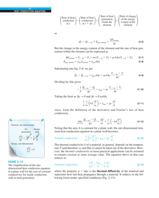
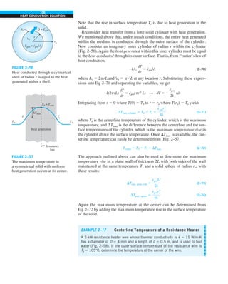
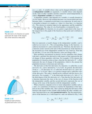
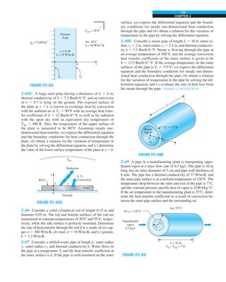
FIGURE 1–42
Although there are three mechanisms
of heat transfer, a medium may
involve only two of them
simultaneously.
Opaque
solid
Conduction
1 mode
T1
T2
Gas
Radiation
Conduction or
convection
2 modes
T1
T2
Vacuum
Radiation 1 mode
T1
T2](https://image.slidesharecdn.com/25489135-230110133727-3d40a16a/85/25489135-pdf-53-320.jpg)
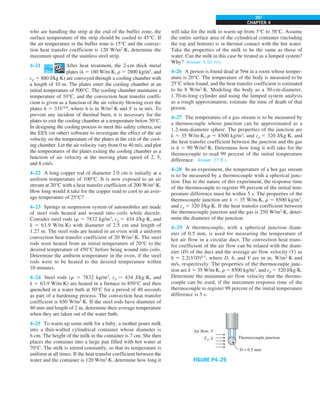
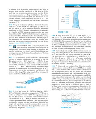
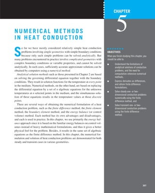
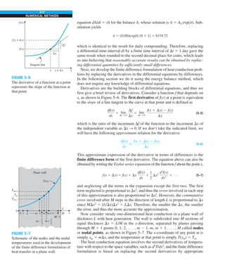
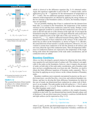
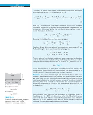
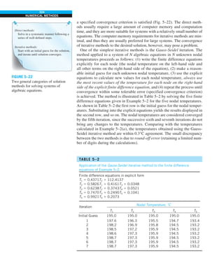
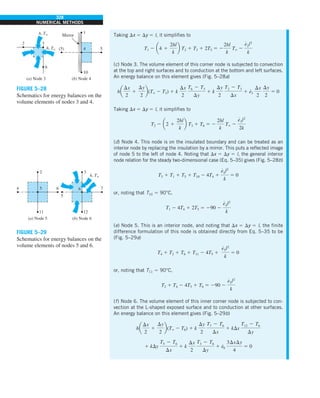
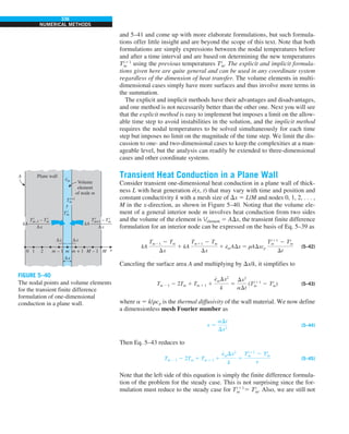
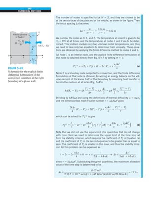
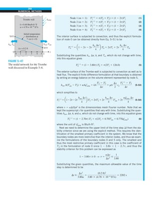
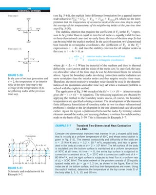
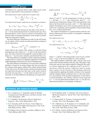
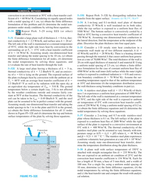
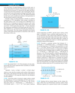
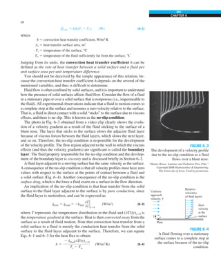
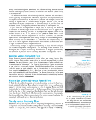
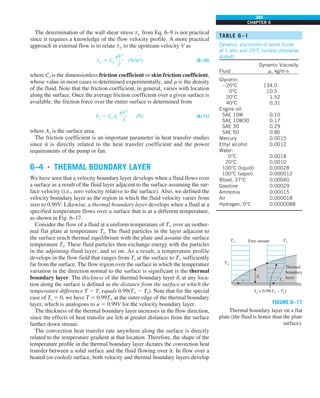
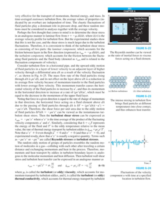
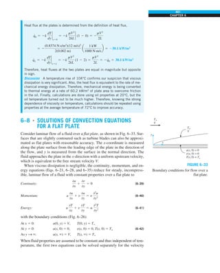
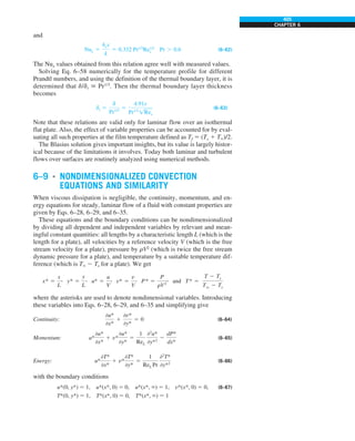
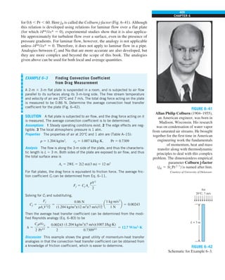
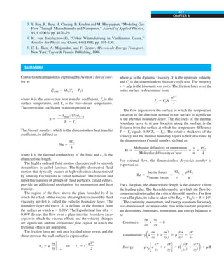
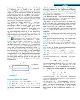
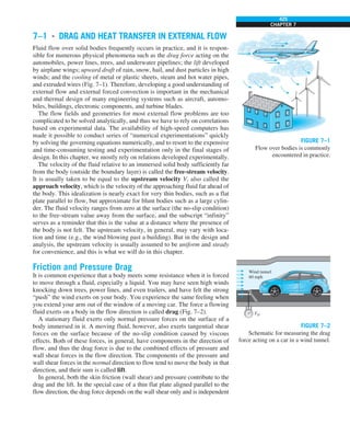
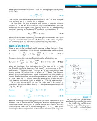
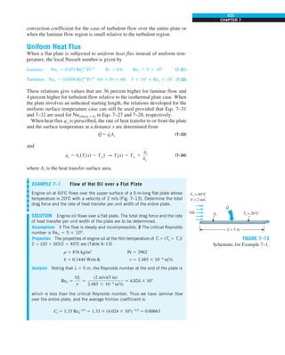
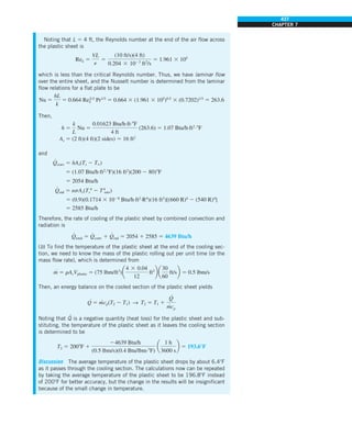
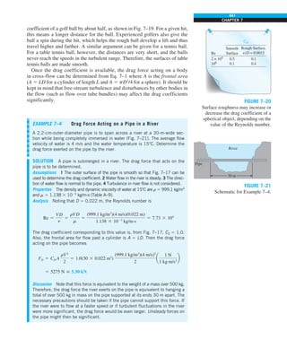
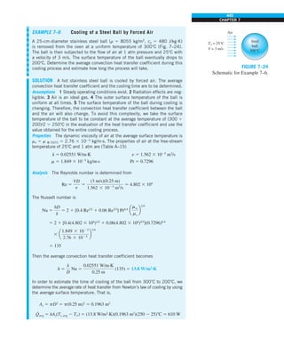
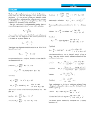
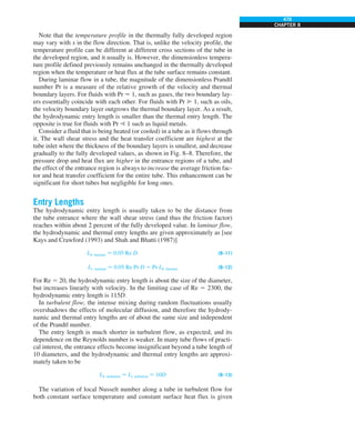
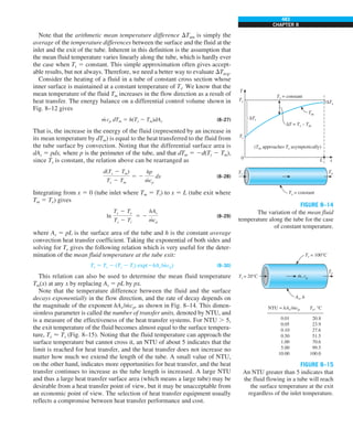
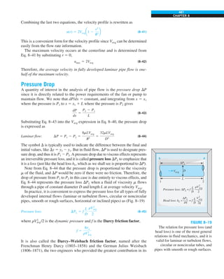
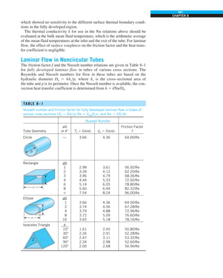
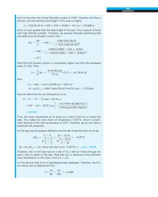
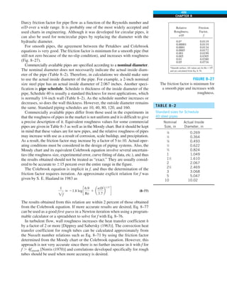
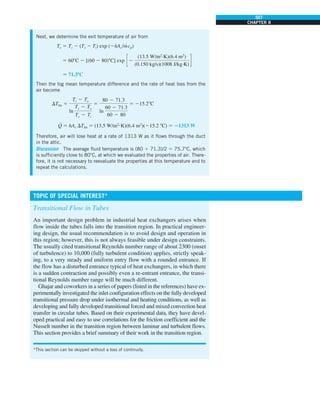
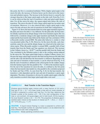
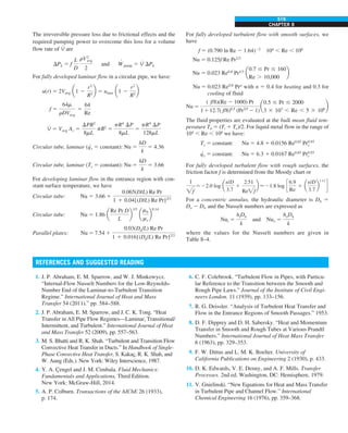
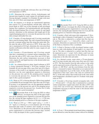
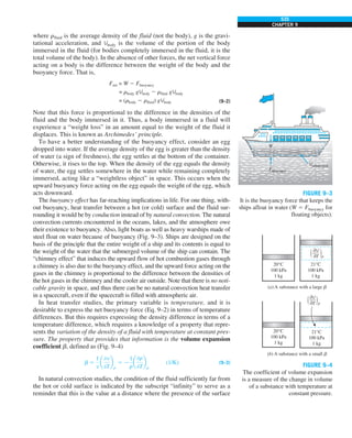
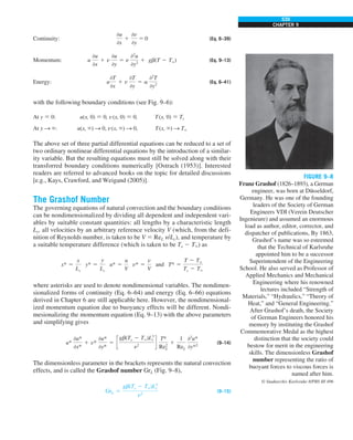
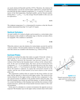
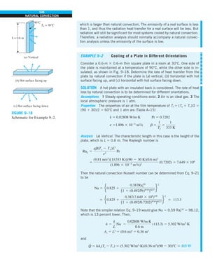
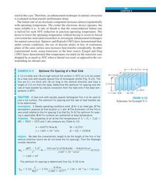
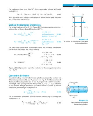
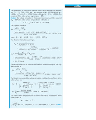
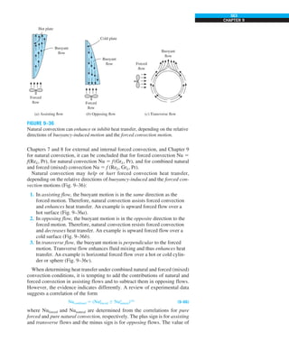
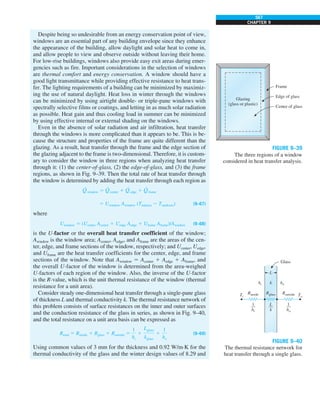
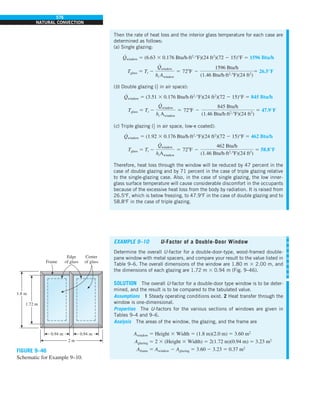
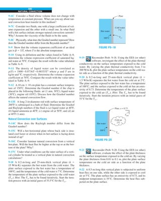
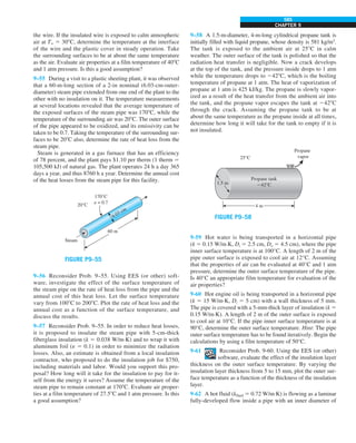
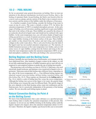
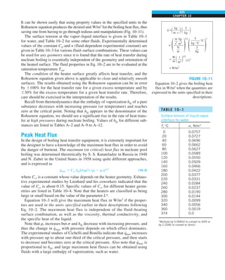
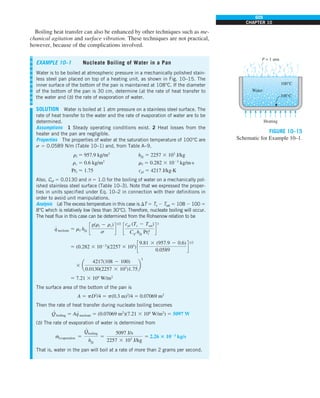
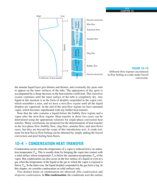
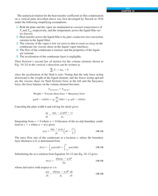
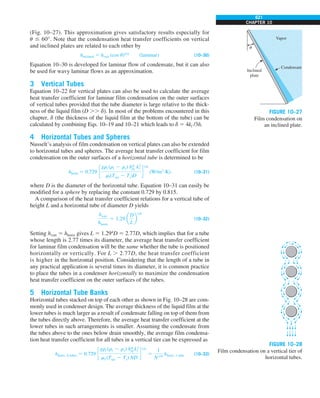
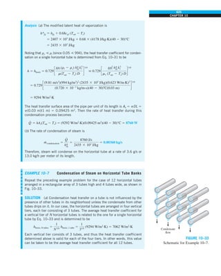
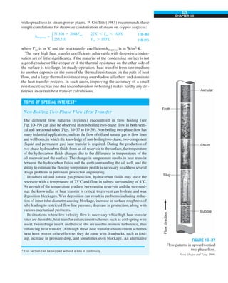
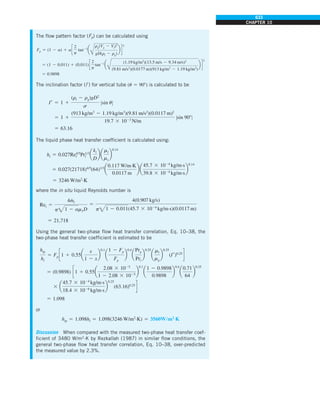
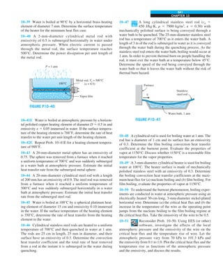
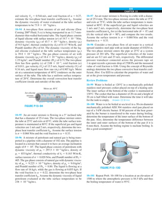
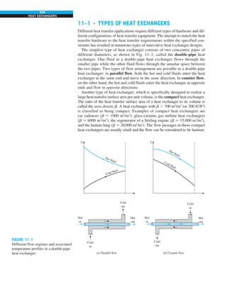
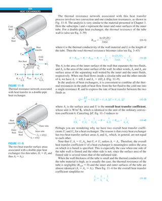
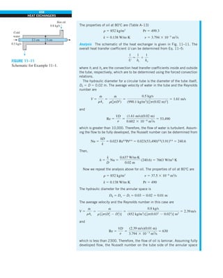
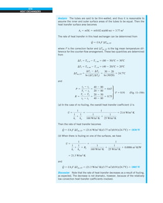
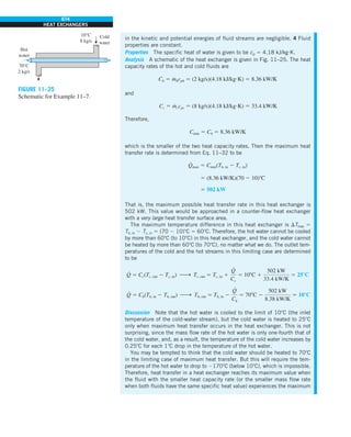
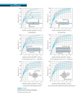
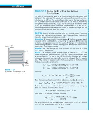
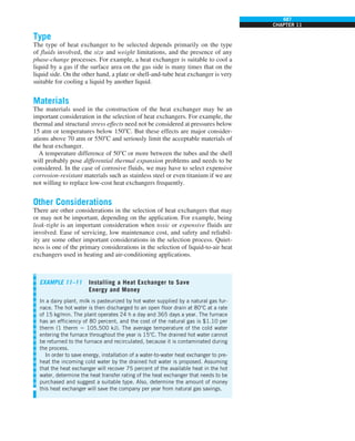
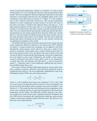
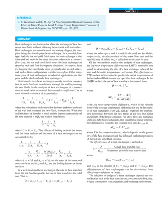
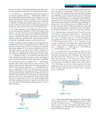
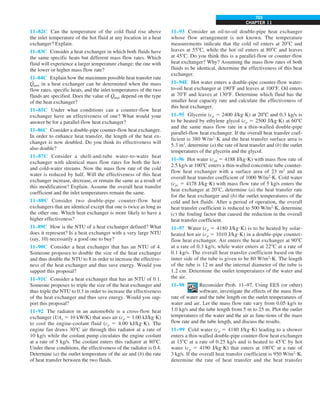
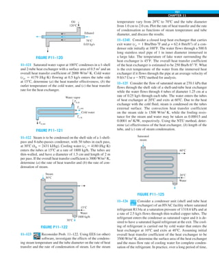
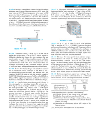
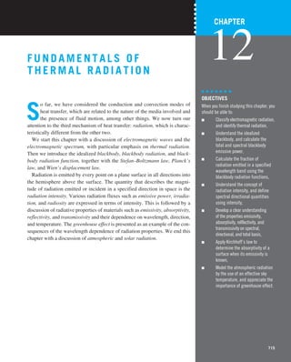
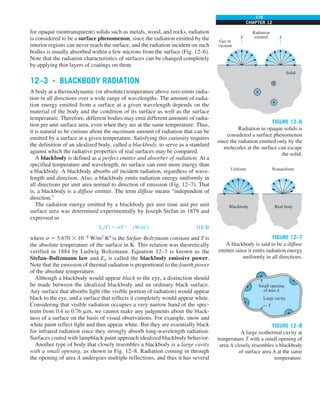
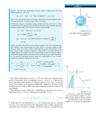
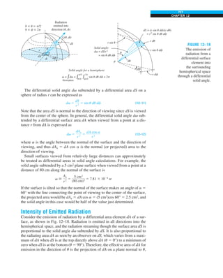
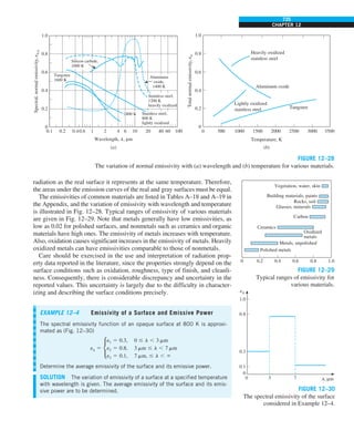
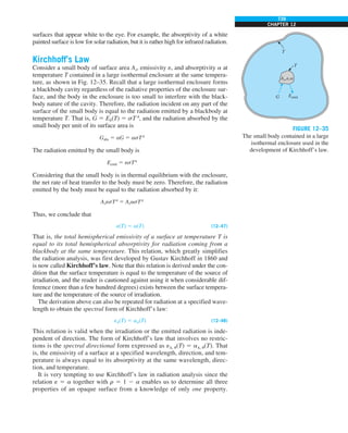
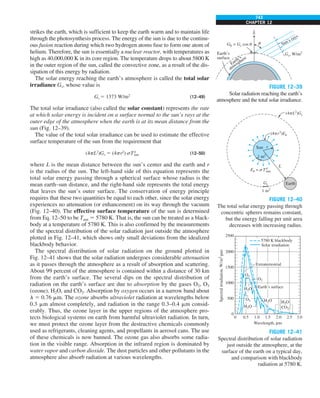
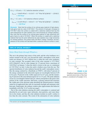
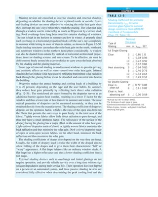
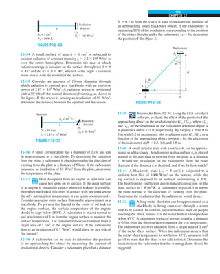
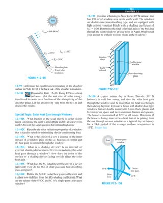
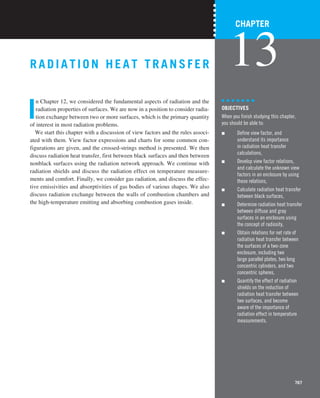
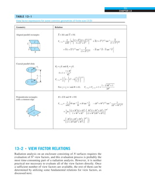
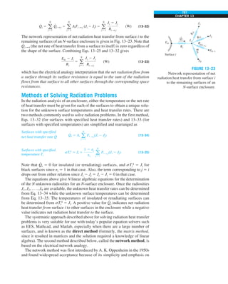
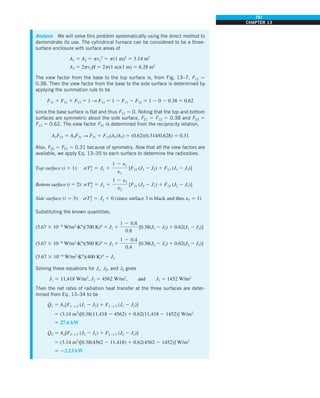
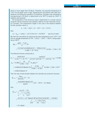
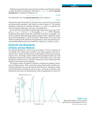
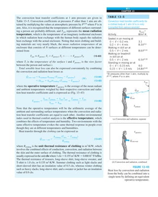
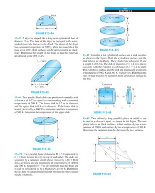
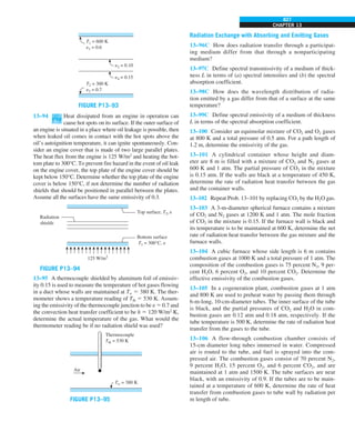
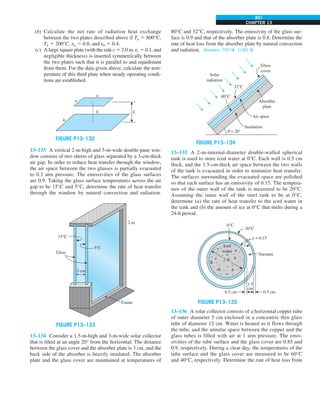
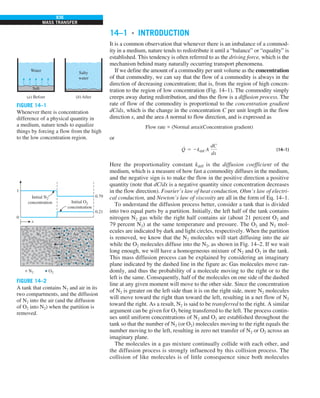
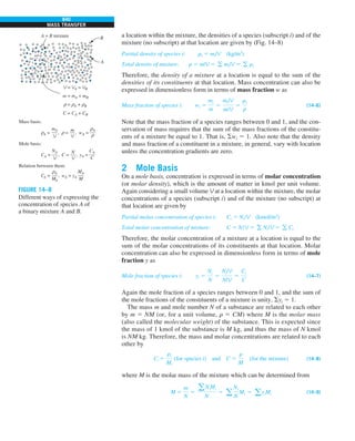
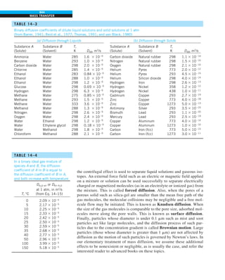
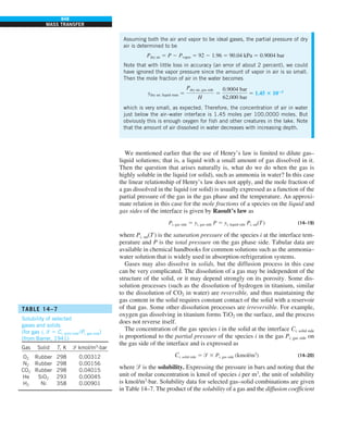
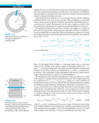
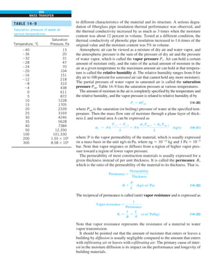
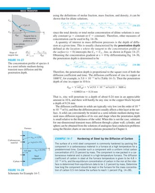
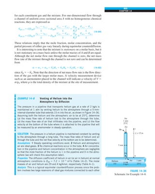
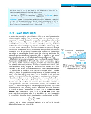
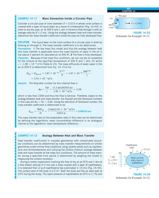
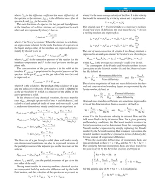
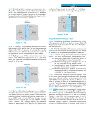
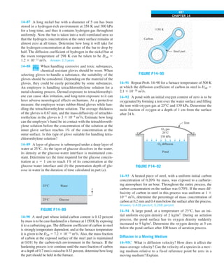
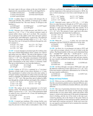
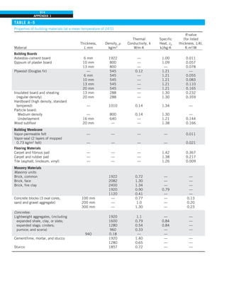
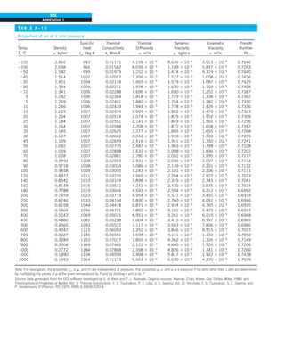
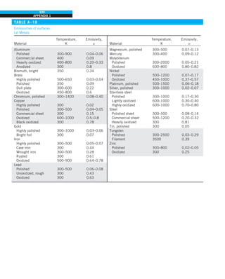
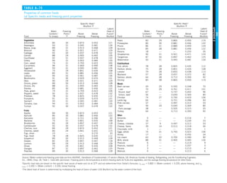
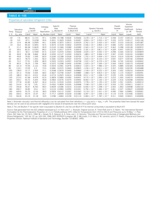
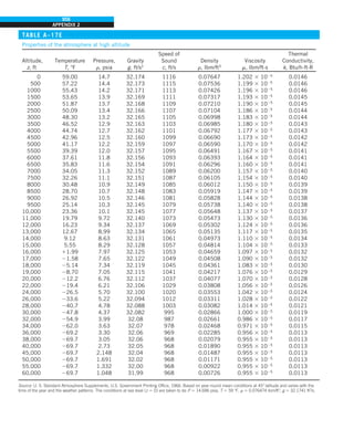
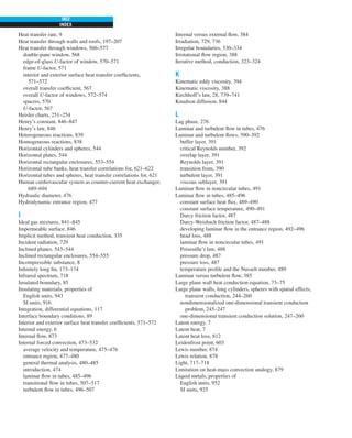
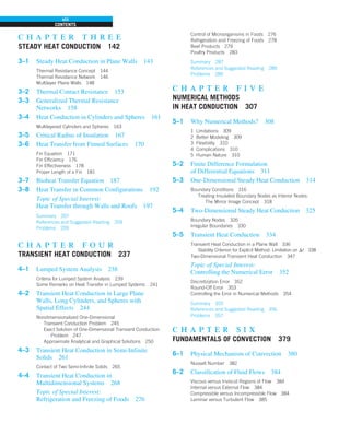
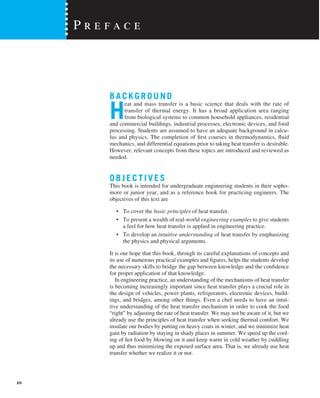
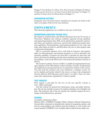
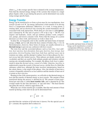
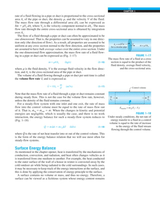
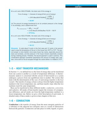
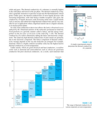
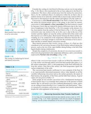
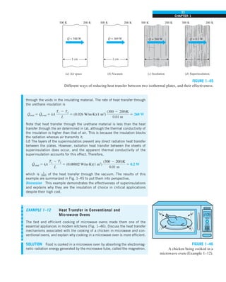
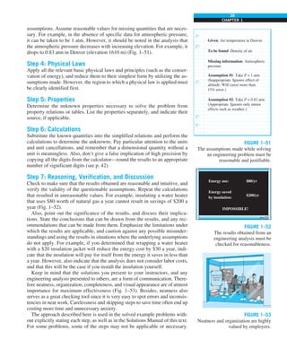
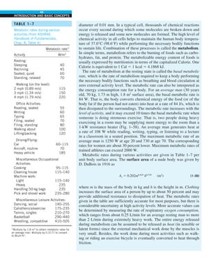
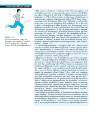
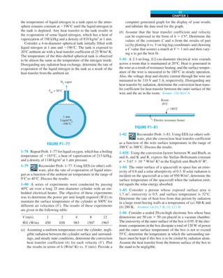
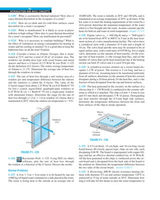
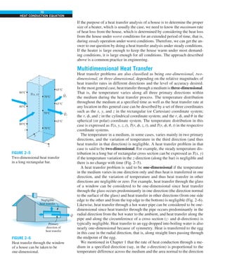
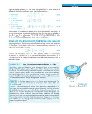
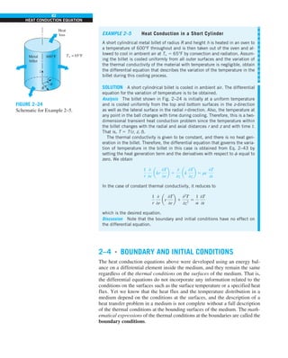
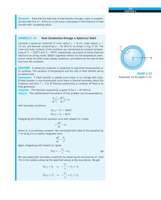
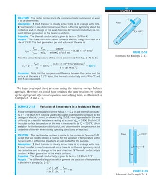
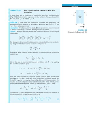
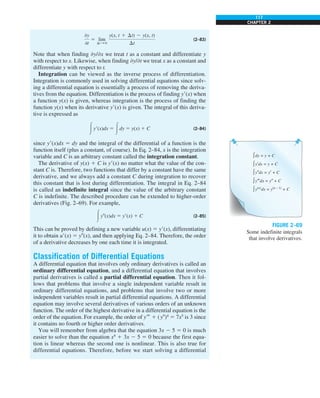
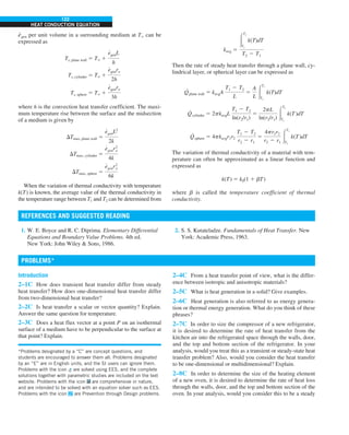
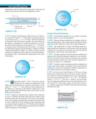
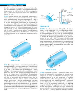
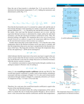
![31
CHAPTER 1
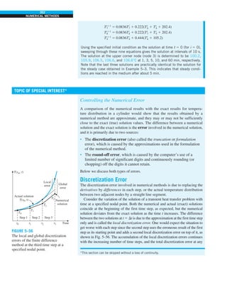
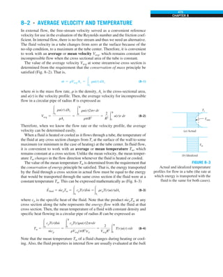
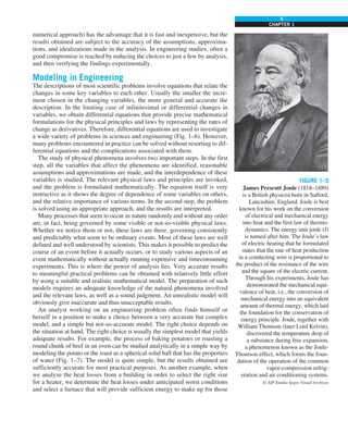
FIGURE 1–43
Heat transfer from the person
described in Example 1–10.
Qcond
·
Room
air
29°C
20°C
Qrad
·
Qconv
·
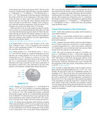
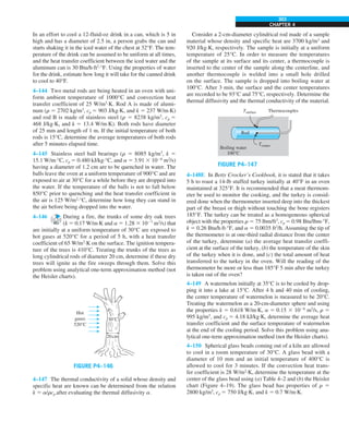
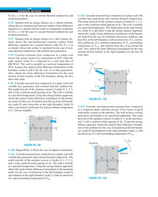
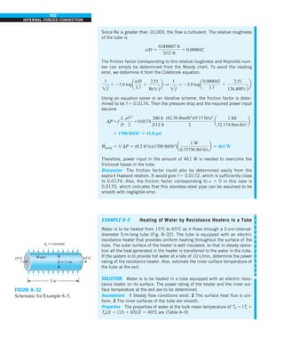
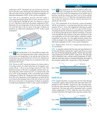
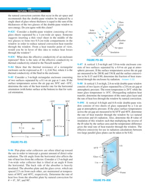
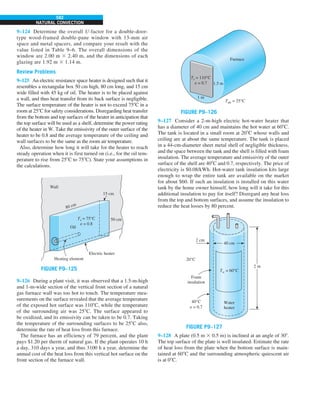
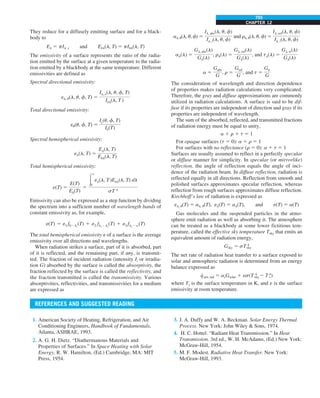
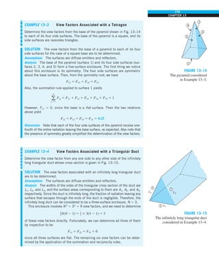
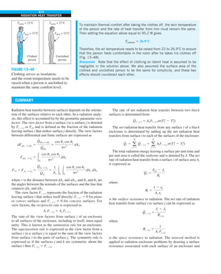
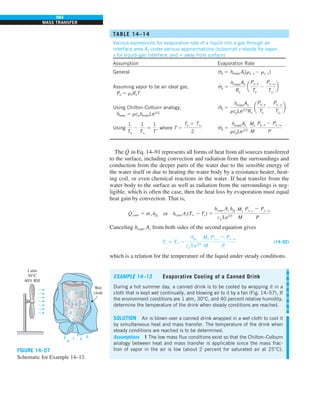
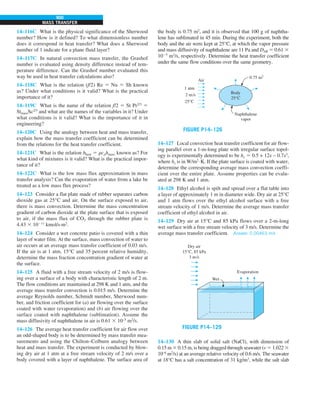
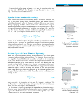
EXAMPLE 1–10 Heat Loss from a Person
Consider a person standing in a breezy room at 20°C. Determine the total rate
of heat transfer from this person if the exposed surface area and the average
outer surface temperature of the person are 1.6 m2
and 29°C, respectively,
and the convection heat transfer coefficient is 6 W/m2
·K (Fig. 1–43).
SOLUTION The total rate of heat transfer from a person by both convection
and radiation to the surrounding air and surfaces at specified temperatures is
to be determined.
Assumptions 1 Steady operating conditions exist. 2 The person is completely
surrounded by the interior surfaces of the room. 3 The surrounding surfaces
are at the same temperature as the air in the room. 4 Heat conduction to the
floor through the feet is negligible.
Properties The emissivity of a person is e 5 0.95 (Table 1–6).
Analysis The heat transfer between the person and the air in the room is by
convection (instead of conduction) since it is conceivable that the air in the
vicinity of the skin or clothing warms up and rises as a result of heat trans-
fer from the body, initiating natural convection currents. It appears that the
experimentally determined value for the rate of convection heat transfer in
this case is 6 W per unit surface area (m2
) per unit temperature difference
(in K or °C) between the person and the air away from the person. Thus, the
rate of convection heat transfer from the person to the air in the room is
Q
·
conv 5 hAs (Ts 2 T∞)
5 (6 W/m2
·K)(1.6 m2
)(29 2 20)°C
5 86.4 W
The person also loses heat by radiation to the surrounding wall surfaces.
We take the temperature of the surfaces of the walls, ceiling, and floor to be
equal to the air temperature in this case for simplicity, but we recognize that
this does not need to be the case. These surfaces may be at a higher or lower
temperature than the average temperature of the room air, depending on the
outdoor conditions and the structure of the walls. Considering that air does
not intervene with radiation and the person is completely enclosed by the sur-
rounding surfaces, the net rate of radiation heat transfer from the person to the
surrounding walls, ceiling, and floor is
Q
·
rad 5 esAs (T 4
s 2 T 4
surr)
5 (0.95)(5.67 3 1028
W/m2
·K4
)(1.6 m2
)
3 [(29 1 273)4
2 (20 1 273)4
] K4
5 81.7 W
Note that we must use thermodynamic temperatures in radiation calculations.
Also note that we used the emissivity value for the skin and clothing at room
temperature since the emissivity is not expected to change significantly at a
slightly higher temperature.
Then the rate of total heat transfer from the body is determined by adding
these two quantities:
Q
·
total 5 Q
·
conv 1 Q
·
rad 5 (86.4 1 81.7) W 168 W](https://image.slidesharecdn.com/25489135-230110133727-3d40a16a/85/25489135-pdf-54-320.jpg)
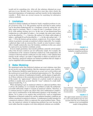
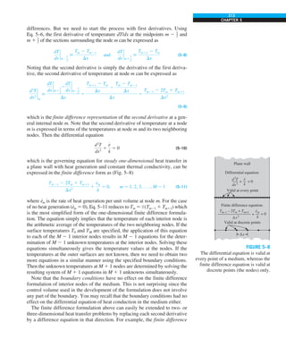
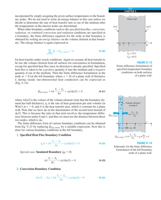
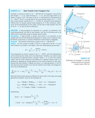
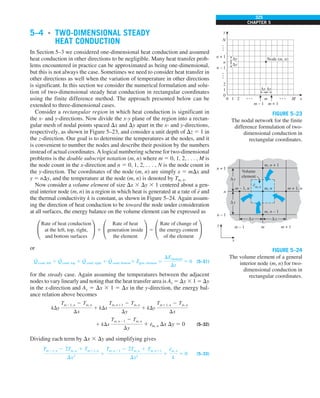
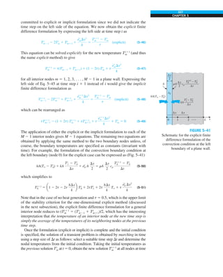
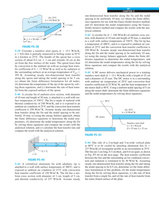
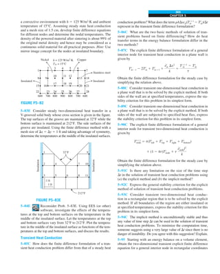
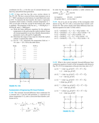
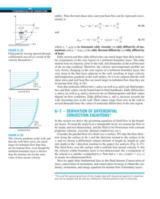
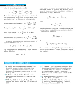
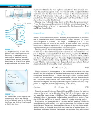
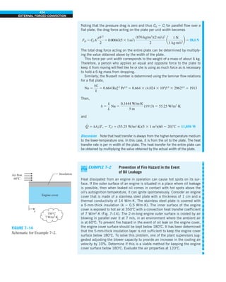
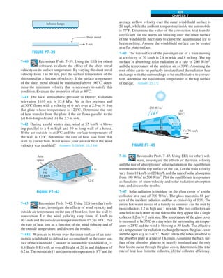
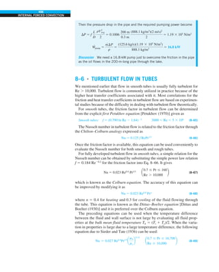
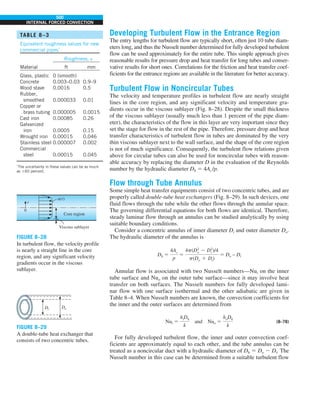
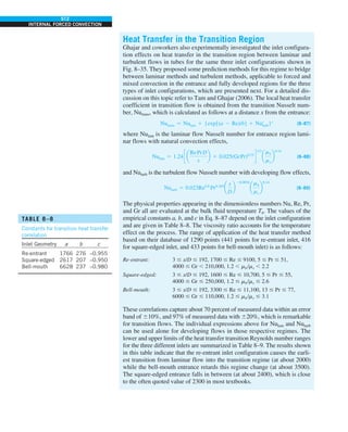
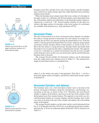
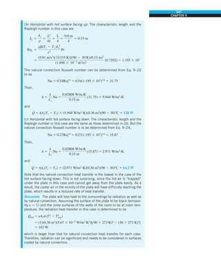
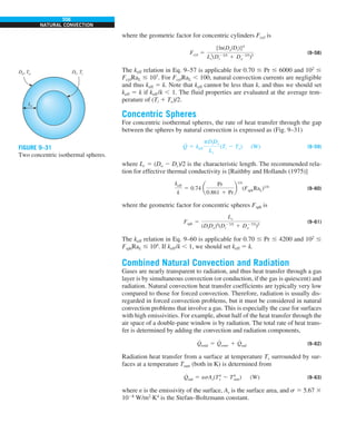
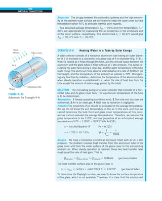
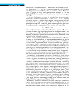
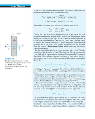
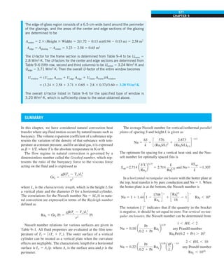
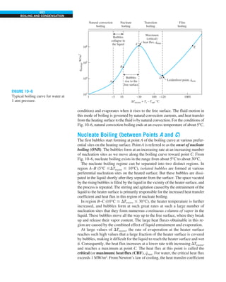
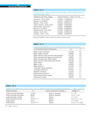
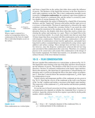
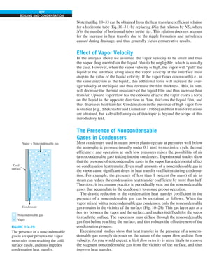
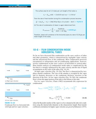
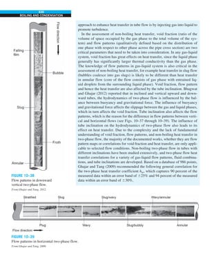
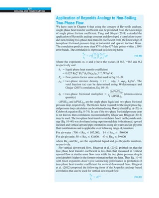
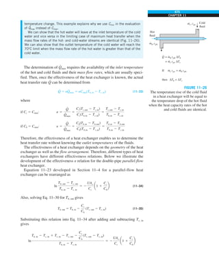
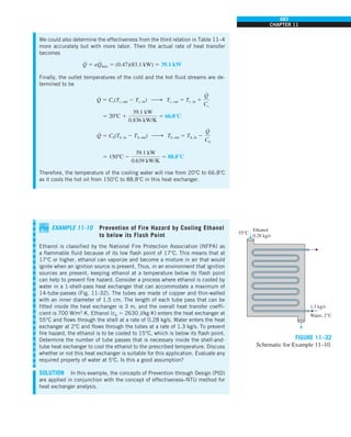
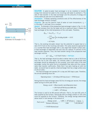
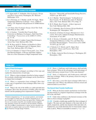
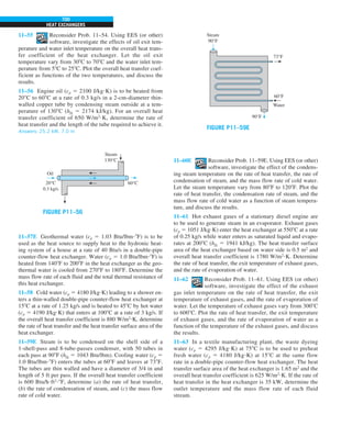
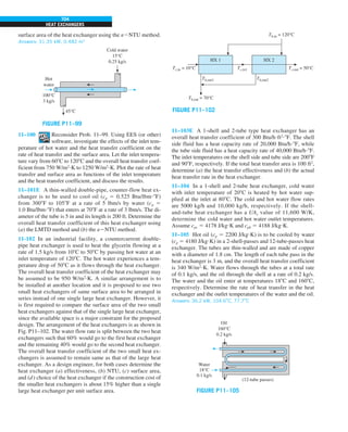
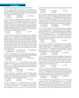
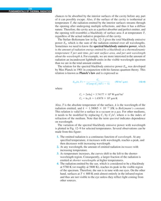
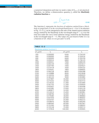
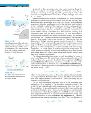
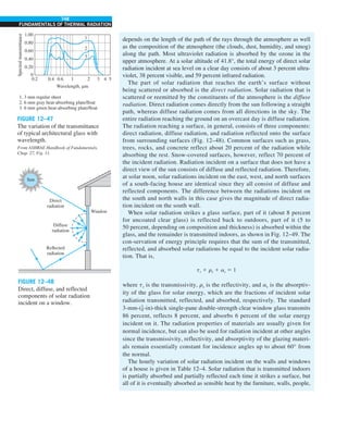
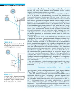
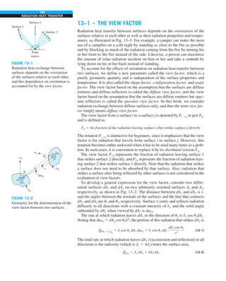
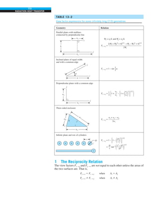
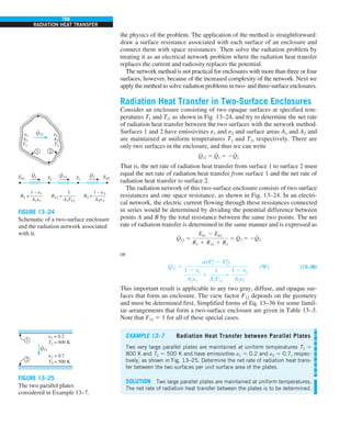
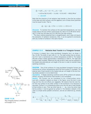
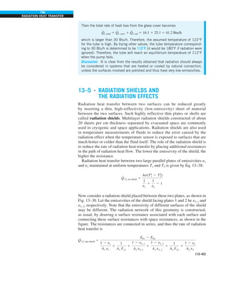
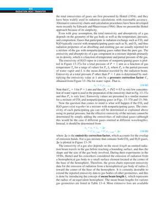
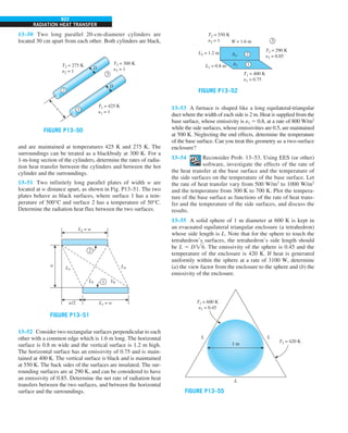
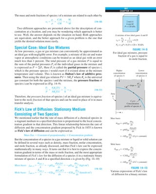
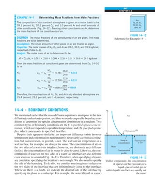
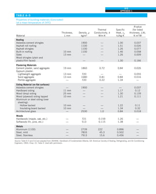
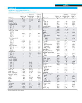
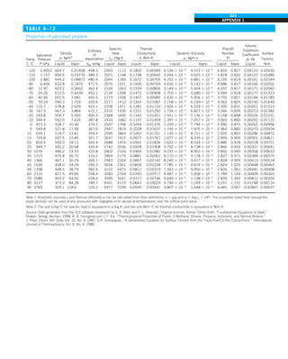
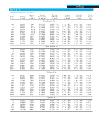
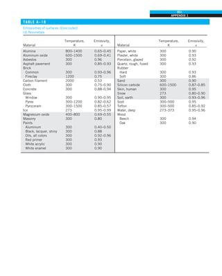
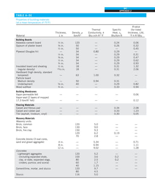
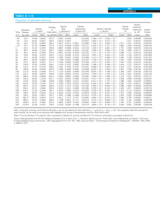
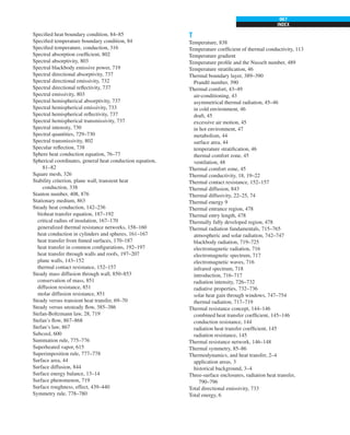
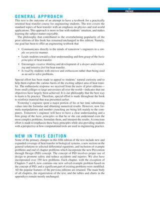
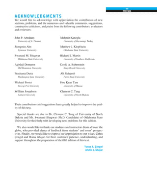
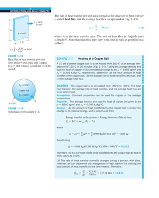
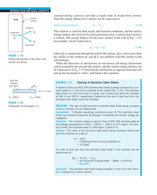
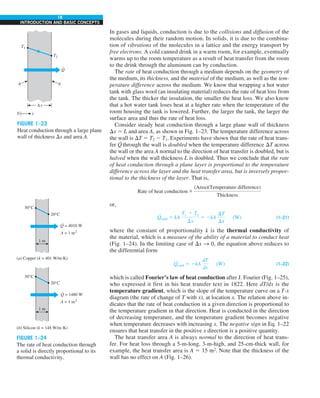
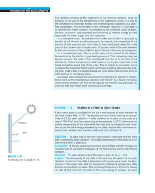
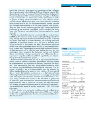
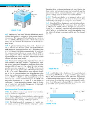
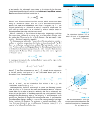
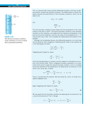
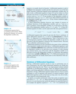
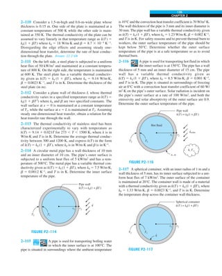
![32
INTRODUCTION AND BASIC CONCEPTS
Discussion The heat transfer would be much higher if the person were not
dressed since the exposed surface temperature would be higher. Thus, an
important function of the clothes is to serve as a barrier against heat transfer.
In these calculations, heat transfer through the feet to the floor by conduc-
tion, which is usually very small, is neglected. Heat transfer from the skin by
perspiration, which is the dominant mode of heat transfer in hot environments,
is not considered here.
Also, the units W/m2
·°C and W/m2
·K for heat transfer coefficient are equiva-
lent, and can be interchanged.
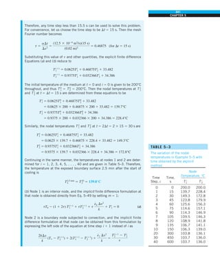
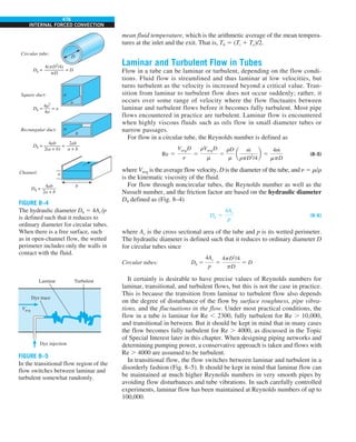
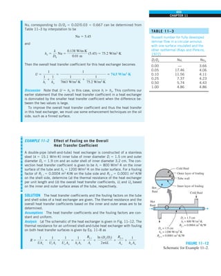
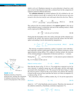
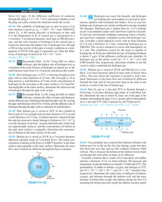
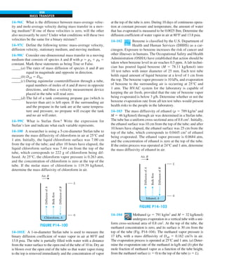
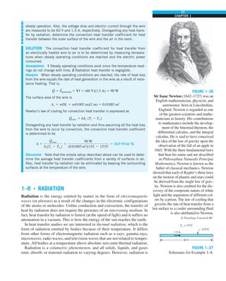
FIGURE 1–44
Schematic for Example 1–11.
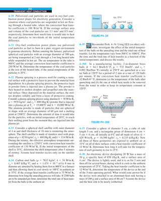
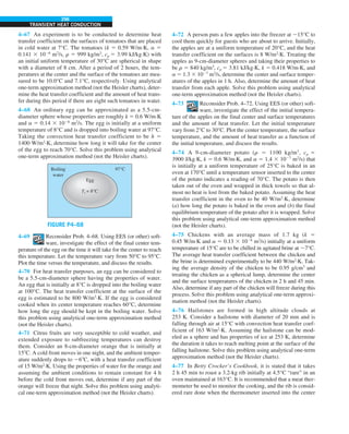
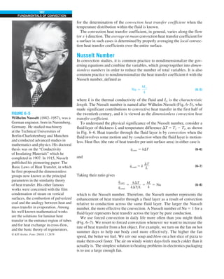
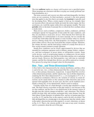
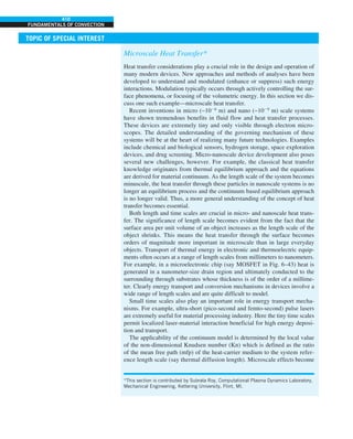
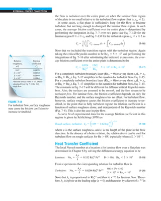
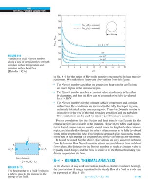
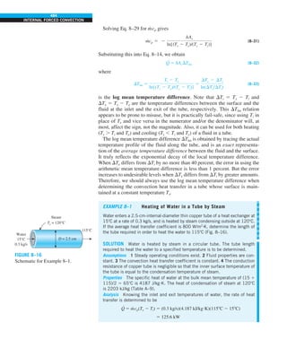
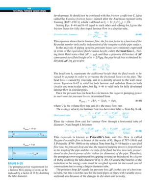
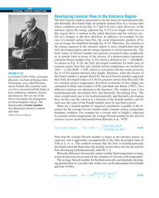
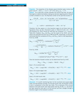
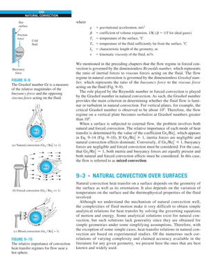
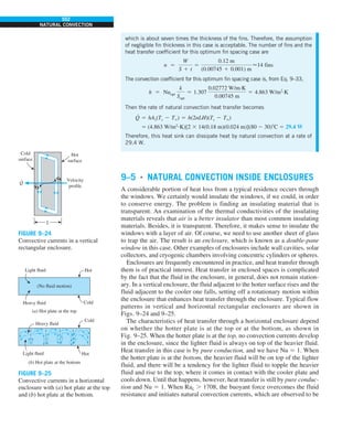
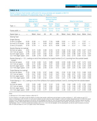
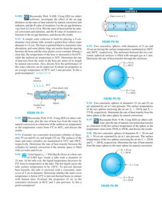
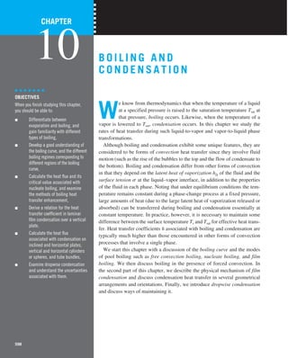
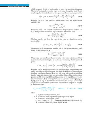
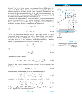
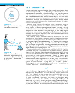
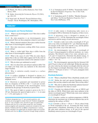
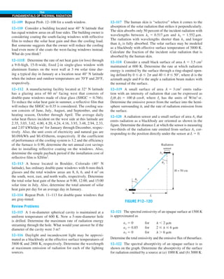
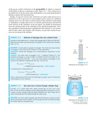
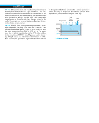
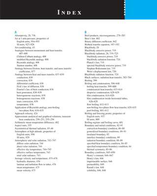
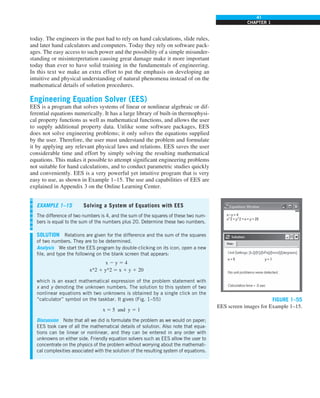
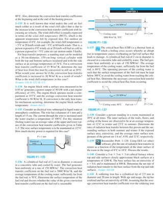
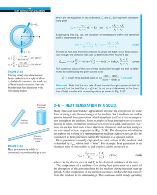
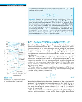
EXAMPLE 1–11 Heat Transfer between Two Isothermal Plates
Consider steady heat transfer between two large parallel plates at constant tem-
peratures of T1 5 300 K and T2 5 200 K that are L 5 1 cm apart, as shown in
Fig. 1–44. Assuming the surfaces to be black (emissivity e 5 1), determine the
rate of heat transfer between the plates per unit surface area assuming the gap
between the plates is (a) filled with atmospheric air, (b) evacuated, (c) filled
with urethane insulation, and (d) filled with superinsulation that has an appar-
ent thermal conductivity of 0.00002 W/m·K.
SOLUTION The total rate of heat transfer between two large parallel plates at
specified temperatures is to be determined for four different cases.
Assumptions 1 Steady operating conditions exist. 2 There are no natural con-
vection currents in the air between the plates. 3 The surfaces are black and
thus e 5 1.
Properties The thermal conductivity at the average temperature of 250 K is
k 5 0.0219 W/m·K for air (Table A–15), 0.026 W/m·K for urethane insulation
(Table A–6), and 0.00002 W/m·K for the superinsulation.
Analysis (a) The rates of conduction and radiation heat transfer between the
plates through the air layer are
Q
·
cond 5 kA
T1 2 T2
L
5 (0.0219 W/m·K)(1 m2
)
(300 2 200)K
0.01 m
5 219 W
and
Q
·
rad 5 esA(T 4
1 2 T 4
2)
5 (1)(5.67 3 1028
W/m2
·K4
)(1 m2
)[(300 K)4
2 (200 K)4
] 5 369 W
Therefore,
Q
·
total 5 Q
·
cond 1 Q
·
rad 5 219 1 369 5 588 W
The heat transfer rate in reality will be higher because of the natural convec-
tion currents that are likely to occur in the air space between the plates.
(b) When the air space between the plates is evacuated, there will be no con-
duction or convection, and the only heat transfer between the plates will be by
radiation. Therefore,
Q
·
total 5 Q
·
rad 5 369 W
(c) An opaque solid material placed between two plates blocks direct radiation
heat transfer between the plates. Also, the thermal conductivity of an insulat-
ing material accounts for the radiation heat transfer that may be occurring
T2
= 200 K
T1
= 300 K
ε = 1
L = 1 cm
Q
·](https://image.slidesharecdn.com/25489135-230110133727-3d40a16a/85/25489135-pdf-55-320.jpg)
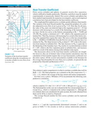
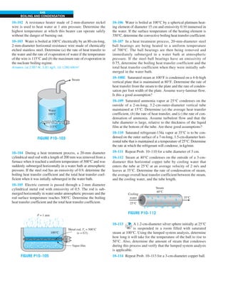
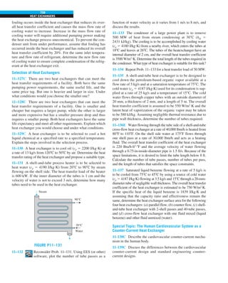
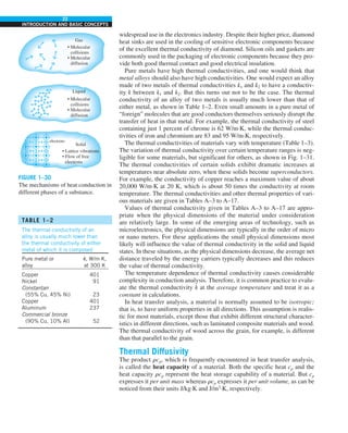
![37
CHAPTER 1
greater than the rate of heat lost to the surroundings. Factors influencing the
autoignition temperature include atmospheric pressure, humidity, and oxygen
concentration.
The science of heat and mass transfer can be coupled with the concepts
of PtD to mitigate the risks of thermal failure in systems. Thermal stress
can compromise the integrity of parts and components in a system. Extreme
temperature can alter the physical properties of a material, which can cause
a component to lose its functionality. Cold temperature on the morning of
January 28, 1986 affected the elasticity of the O-ring on a solid rocket booster
of the space shuttle Challenger. The loss of the O-ring’s elasticity and abil-
ity to seal allowed hot combustion gas to leak through a solid rocket booster,
which led to the tragic disaster.
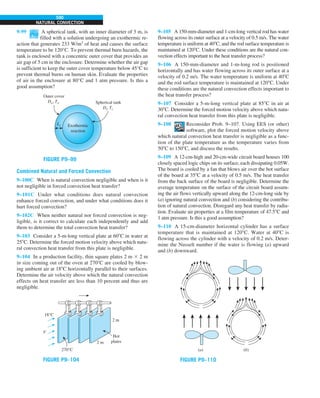
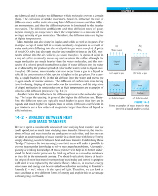
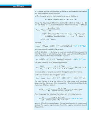
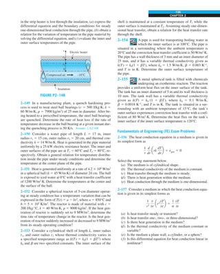
EXAMPLE 1–14 Fire Hazard Prevention of Oil Leakage on
Hot Engine Surface
Oil leakage and spillage on hot engine surface can lead to fire hazards. Some
engine oils have an autoignition temperature of approximately above 250°C.
When oil leakage comes in contact with a hot engine surface that has a higher
temperature than its autoignition temperature, the oil can ignite spontane-
ously. Consider the outer surface of an engine situated in a place where there
is a possibility of being in contact with oil leakage. The engine surface has an
emissivity of 0.3, and when it is in operation, its inner surface is subjected
to 5 kW/m2
of heat flux. The engine is in an environment where the ambient
air and surrounding temperature is 40°C, while the convection heat transfer
coefficient is 15 W/m2
∙K. To prevent a fire hazard in the event of oil leakage
being in contact with the engine surface, the temperature of the engine sur-
face should be kept below 200°C. Determine whether oil leakage drops on the
engine surface are at a risk of autoignition. If there is a risk of autoignition,
discuss a possible prevention measure that can be implemented.
SOLUTION In this example, the concepts of PtD are applied with the basic
understanding of simultaneous heat transfer mechanisms via convection and
radiation. The inner surface of an engine is subject to a heat flux of 5 kW/m2
.
The engine surface temperature is to be determined whether it is below 200°C,
to prevent spontaneous ignition in the event of oil leakage drops on the engine
surface.
Assumptions 1 Steady operating conditions exist. 2 The surrounding surfaces
are at the same temperature as the ambient air. 3 Heat conduction through the
engine housing is one-dimensional. 4 The engine inner surface is subjected to
uniform heat flux.
Properties Emissivity of the engine surface is given as « 5 0.3.
Analysis When in operation, the inner surface of the engine is subjected to
a uniform heat flux, which is equal to the sum of heat fluxes transferred by
convection and radiation on the outer surface. Therefore,
q
·
0 5 h(To 2 T∞) 1 es(T 4
o 2 T 4
surr)
5000 W/m2
5 (15 W/m2
·K)[To 2 (40 1 273)]K
1(0.3)(5.67 3 1028
W/m2
·K4
)[T 4
o 2 (40 1 273)4
]K4
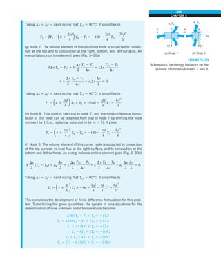
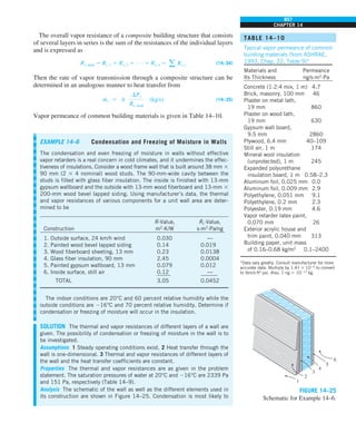
FIGURE 1–49
Schematic for Example 1–14
Air, 40°C
h = 15 W/m2
·K
Engine housing
e = 0.3
q0 = 5 kW/m2
.
To 200°C
Tsurr = 40°C](https://image.slidesharecdn.com/25489135-230110133727-3d40a16a/85/25489135-pdf-60-320.jpg)
![38
INTRODUCTION AND BASIC CONCEPTS
The engine outer surface temperature (T0) can be solved implicitly using the
Engineering Equation Solver (EES) software that accompanies this text with
the following lines:
h515 [W/m^2-K]
q_dot_055000 [W/m^2]
T_surr5313 [K]
epsilon50.3
sigma55.67e-8 [W/m^2-K^4]
q_dot_05h*(T_o-T_surr)+epsilon*sigma#*(T_o^4-T_surr^4)
The engine outer surface temperature is found to be To 5 552 K 5 279°C
Discussion The solution reveals that the engine outer surface temperature is
greater than 200°C, the temperature required to prevent the risk of autoigni-
tion in the event of oil leakage drops on the engine outer surface. To mitigate
the risk of fire hazards, the outer surface of the engine should be insulated.
In practice, the engine surface temperature is not uniform; instead, high local
surface temperatures result in hot spots on the engine surface. Engine hous-
ings generally come in irregular shapes, thus making the prediction of hot
spots on the engine surface difficult. However, using handheld infrared ther-
mometers, engine operators can quickly identify the approximate areas that
are prone to hot spots and take proper prevention measures.
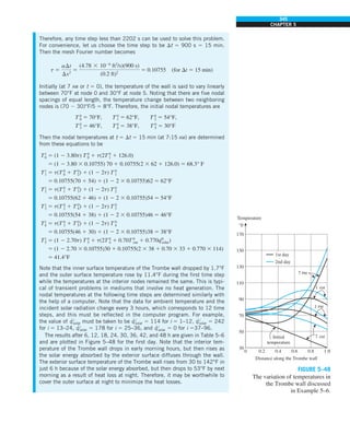
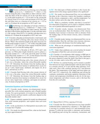
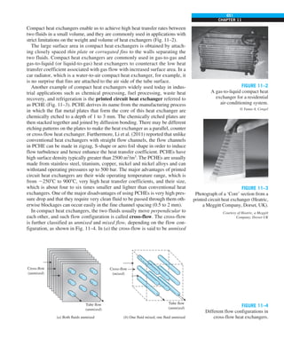
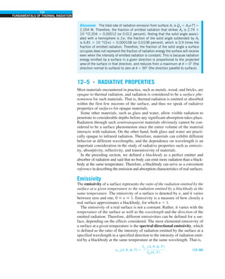
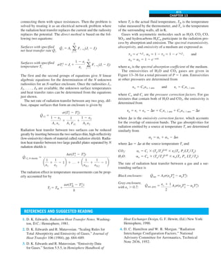
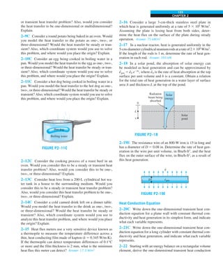
FIGURE 1–50
A step-by-step approach can greatly
simplify problem solving.
Solution
Hard
way
Easy way
Problem
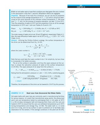
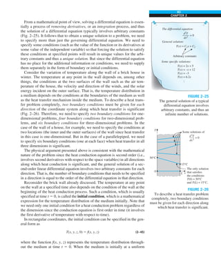
1–11 ■
PROBLEM-SOLVING TECHNIQUE
The first step in learning any science is to grasp the fundamentals and to gain
a sound knowledge of it. The next step is to master the fundamentals by test-
ing this knowledge. This is done by solving significant real-world problems.
Solving such problems, especially complicated ones, requires a systematic
approach. By using a step-by-step approach, an engineer can reduce the solu-
tion of a complicated problem into the solution of a series of simple problems
(Fig. 1–50). When you are solving a problem, we recommend that you use the
following steps zealously as applicable. This will help you avoid some of the
common pitfalls associated with problem solving.
Step 1: Problem Statement
In your own words, briefly state the problem, the key information given, and
the quantities to be found. This is to make sure that you understand the prob-
lem and the objectives before you attempt to solve the problem.
Step 2: Schematic
Draw a realistic sketch of the physical system involved, and list the relevant
information on the figure. The sketch does not have to be something elab-
orate, but it should resemble the actual system and show the key features.
Indicate any energy and mass interactions with the surroundings. Listing the
given information on the sketch helps one to see the entire problem at once.
Step 3: Assumptions and Approximations
State any appropriate assumptions and approximations made to simplify the
problem to make it possible to obtain a solution. Justify the questionable](https://image.slidesharecdn.com/25489135-230110133727-3d40a16a/85/25489135-pdf-61-320.jpg)

![CHAPTER 1
55
inner surface to 74°C at the outer surface. Determine the ther-
mal conductivity of the material at the average temperature.
FIGURE P1–59
Insulation
Insulation
Wattmeter
Source
Resistance
heater
Samples
0.5 cm
~
1–60 Silicon wafer is susceptible to warping when the
wafer is subjected to temperature difference
across its thickness. Thus, steps needed to be taken to prevent
the temperature gradient across the wafer thickness from get-
ting large. As an engineer in a semiconductor company, your
task is to determine the maximum allowable heat flux on the
bottom surface of the wafer, while maintaining the upper sur-
face temperature at 27°C. To prevent the wafer from warp-
ing, the temperature difference across its thickness of 500 mm
cannot exceed 1°C.
q
.
L = 500 μm
Silicon wafer
Tup
Tbot
FIGURE P1–60
1–61 A concrete wall with a surface area of 20 m2
and a thick-
ness of 0.30 m separates conditioned room air from ambient
air. The temperature of the inner surface of the wall (T1) is
maintained at 25ºC. (a) Determine the heat loss Q
·
(W) through
the concrete wall for three thermal conductivity values of
(0.75, 1, and 1.25 W/m·K) and outer wall surface temperatures
of T2 5 215, 210, 25, 0, 5, 10, 15, 20, 25, 30, and 38 ºC
(a total of 11 data points for each thermal conductivity value).
Tabulate the results for all three cases in one table. Also pro-
vide a computer generated graph [Heat loss, Q
·
(W) vs. Outside
wall temperature, T2 (ºC)] for the display of your results. The
results for all three cases should be plotted on the same graph.
(b) Discuss your results for the three cases.
1–62 A hollow spherical iron container with outer diameter
20 cm and thickness 0.2 cm is filled with iced water at 0°C.
If the outer surface temperature is 5°C, determine the approx-
imate rate of heat loss from the sphere, in kW, and the rate at
which ice melts in the container. The heat of fusion of water
is 333.7 kJ/kg.
FIGURE P1–62
0.2 cm
5°C
Iced
water
1–63 Reconsider Prob. 1–62. Using EES (or other)
software, plot the rate at which ice melts as a func-
tion of the container thickness in the range of 0.1 cm to
1.0 cm. Discuss the results.
1–64E The inner and outer glasses of a 4-ft 3 4-ft double-
pane window are at 60°F and 48°F, respectively. If the 0.25-in.
space between the two glasses is filled with still air, determine
the rate of heat transfer through the window.
Answer: 131 Btu/h
1–65E An engineer who is working on the heat transfer
analysis of a house in English units needs the convection
heat transfer coefficient on the outer surface of the house.
But the only value he can find from his handbooks is
22 W/m2
·K, which is in SI units. The engineer does not have
a direct conversion factor between the two unit systems for
the convection heat transfer coefficient. Using the conver-
sion factors between W and Btu/h, m and ft, and °C and °F,
express the given convection heat transfer coefficient in Btu/
h·ft2
·°F. Answer: 3.87 Btu/h·ft2
·°F
1–66 Air at 20ºC with a convection heat transfer coefficient
of 20 W/m2
·K blows over a pond. The surface temperature of
the pond is at 40ºC. Determine the heat flux between the sur-
face of the pond and the air.
1–67 Four power transistors, each dissipating 12 W, are
mounted on a thin vertical aluminum plate 22 cm 3 22 cm in
size. The heat generated by the transistors is to be dissipated
by both surfaces of the plate to the surrounding air at 25°C,
which is blown over the plate by a fan. The entire plate can be
assumed to be nearly isothermal, and the exposed surface area
of the transistor can be taken to be equal to its base area. If the
average convection heat transfer coefficient is 25 W/m2
·K,
determine the temperature of the aluminum plate. Disregard
any radiation effects.
1–68 In a power plant, pipes transporting superheated vapor
are very common. Superheated vapor is flowing at a rate of
0.3 kg/s inside a pipe with 5 cm in diameter and 10 m in length.
The pipe is located in a power plant at 20°C, and has a uniform](https://image.slidesharecdn.com/25489135-230110133727-3d40a16a/85/25489135-pdf-78-320.jpg)


5 212 W/cm3
Similarly, heat flux on the outer surface of the wire as a result of this heat
generation is determined by dividing the total rate of heat generation by the
surface area of the wire,
Q
·
s 5
E
#
gen
Awire
5
E
#
gen
pDL
5
1200 W
p(0.3 cm)(80 cm)
5 15.9 W/cm2
Discussion Note that heat generation is expressed per unit volume in W/cm3
or Btu/h·ft3
, whereas heat flux is expressed per unit surface area in W/cm2
or
Btu/h·ft2
.
Hair dryer
1200 W
FIGURE 2–11
Schematic for Example 2–1.
0
Volume
element
A
x
Ax = Ax + Δx = A
L
x
x + Δx
Qx
·
Qx + Δx
·
Egen
·
FIGURE 2–12
One-dimensional heat conduction
through a volume element in
a large plane wall.](https://image.slidesharecdn.com/25489135-230110133727-3d40a16a/85/25489135-pdf-96-320.jpg)
![75
CHAPTER 2
(1) Steady-state:
(−/−t 5 0)
d2
T
dx2
1
e
#
gen
k
5 0 (2–15)
(2) Transient, no heat generation:
(e
·
gen 5 0)
02
T
0x2
5
1
a
0T
0t
(2–16)
(3) Steady-state, no heat generation:
(−/−t 5 0 and e
·
gen 5 0)
d2
T
dx2
5 0 (2–17)
Note that we replaced the partial derivatives by ordinary derivatives in the
one-dimensional steady heat conduction case since the partial and ordinary
derivatives of a function are identical when the function depends on a single
variable only [T 5 T(x) in this case]. For the general solution of Eqs. 2–15
and 2–17 refer to the TOPIC OF SPECIAL INTEREST (A Brief Review of
Differential Equations) at the end of this chapter.
Heat Conduction Equation in a Long Cylinder
Now consider a thin cylindrical shell element of thickness Dr in a long
cylinder, as shown in Fig. 2–14. Assume the density of the cylinder is r, the
specific heat is c, and the length is L. The area of the cylinder normal to the
direction of heat transfer at any location is A 5 2prL where r is the value
of the radius at that location. Note that the heat transfer area A depends on r
in this case, and thus it varies with location. An energy balance on this thin
cylindrical shell element during a small time interval Dt can be expressed as
£
Rate of heat
conduction
at r
≥ 2 £
Rate of heat
conduction
at r 1 Dr
≥ 1 §
Rate of heat
¥ 5 §
Rate of change
¥
generation of the energy
inside the content of the
element element
or
Q
·
r 2 Q
·
r 1 Dr 1 E
·
gen, element 5
DEelement
Dt
(2–18)
The change in the energy content of the element and the rate of heat genera-
tion within the element can be expressed as
DEelement 5 Et 1 Dt 2 Et 5 mc(Tt 1 Dt 2 Tt) 5 rcADr(Tt 1 Dt 2 Tt) (2–19)
E
·
gen, element 5 e
·
genVelement 5 e
·
gen ADr (2–20)
Substituting into Eq. 2–18, we get
Q
·
r 2 Q
·
r 1 Dr 1 e
·
gen ADr 5 rcADr
Tt 1 Dt 2 Tt
Dt
(2–21)
where A 5 2prL. You may be tempted to express the area at the middle of the
element using the average radius as A 5 2p(r 1 Dr/2)L. But there is nothing
we can gain from this complication since later in the analysis we will take the
limit as Dr S 0 and thus the term Dr/2 will drop out. Now dividing the equa-
tion above by ADr gives
2
1
A
Q
#
r 1 Dr 2 Q
#
r
Dr
1 e
·
gen 5 rc
Tt 1 Dt 2 Tt
Dt
(2–22)
L
0
Volume element
r + Δr
r
r
Qr
·
Qr + Δr
·
Egen
·
FIGURE 2–14
One-dimensional heat conduction
through a volume element
in a long cylinder.](https://image.slidesharecdn.com/25489135-230110133727-3d40a16a/85/25489135-pdf-98-320.jpg)
![76
HEAT CONDUCTION EQUATION
Taking the limit as Dr S 0 and Dt S 0 yields
1
A
0
0r
akA
0T
0r
b 1 e
·
gen 5 rc
0T
0t
(2–23)
since, from the definition of the derivative and Fourier’s law of heat conduction,
lim
Dr S 0
Q
#
r1Dr 2 Q
#
r
Dr
5
0Q
#
0r
5
0
0r
a2kA
0T
0r
b (2–24)
Noting that the heat transfer area in this case is A 5 2prL, the one-dimensional
transient heat conduction equation in a cylinder becomes
Variable conductivity:
1
r
0
0r
ark
0T
0r
b 1 e
·
gen 5 rc
0T
0t
(2–25)
For the case of constant thermal conductivity, the previous equation reduces to
Constant conductivity:
1
r
0
0r
ar
0T
0r
b 1
e
#
gen
k
5
1
a
0T
0t
(2–26)
where again the property a 5 k/rc is the thermal diffusivity of the material.
Eq. 2–26 reduces to the following forms under specified conditions (Fig. 2–15):
(1) Steady-state:
(−/−t 5 0)
1
r
d
dr
ar
dT
dr
b 1
e
#
gen
k
5 0 (2–27)
(2) Transient, no heat generation:
(e
·
gen 5 0)
1
r
0
0r
ar
0T
0r
b 5
1
a
0T
0t
(2–28)
(3) Steady-state, no heat generation:
(−/−t 5 0 and e
·
gen 5 0)
d
dr
ar
dT
dr
b 5 0 (2–29)
Note that we again replaced the partial derivatives by ordinary derivatives
in the one-dimensional steady heat conduction case since the partial and or-
dinary derivatives of a function are identical when the function depends on
a single variable only [T 5 T(r) in this case]. For the general solution of
Eqs. 2–27 and 2–29 refer to the TOPIC OF SPECIAL INTEREST (A Brief
Review of Differential Equations) at the end of this chapter.
Heat Conduction Equation in a Sphere
Now consider a sphere with density r, specific heat c, and outer radius R. The
area of the sphere normal to the direction of heat transfer at any location is
A 5 4pr2
, where r is the value of the radius at that location. Note that the heat
transfer area A depends on r in this case also, and thus it varies with location.
By considering a thin spherical shell element of thickness Dr and repeating
the approach described above for the cylinder by using A 5 4pr2
instead of
A 5 2prL, the one-dimensional transient heat conduction equation for a
sphere is determined to be (Fig. 2–16)
Variable conductivity:
1
r2
0
0r
ar2
k
0T
0r
b 1 e
·
gen 5 rc
0T
0t
(2–30)
which, in the case of constant thermal conductivity, reduces to
Constant conductivity:
1
r2
0
0r
ar2
0T
0r
b 1
e
#
gen
k
5
1
a
0T
0t
(2–31)
FIGURE 2–15
Two equivalent forms of the
differential equation for the one-
dimensional steady heat conduction in
a cylinder with no heat generation.
0 R
Volume
element
r + Δr
r r
Qr
·
Qr + Δr
·
Egen
·
FIGURE 2–16
One-dimensional heat conduction
through a volume element in a sphere.
(a) The form that is ready to integrate
(b) The equivalent alternative form
d
dr
dT
dr
r = 0
d2
T
dr2
dT
dr
r = 0
+](https://image.slidesharecdn.com/25489135-230110133727-3d40a16a/85/25489135-pdf-99-320.jpg)

5 0.318 3 109
W/m3
Noting that the thermal conductivity is given to be constant, the differential
equation that governs the variation of temperature in the wire is simply
Eq. 2–27,
1
r
d
dr
ar
dT
dr
b 1
e
#
gen
k
5 0
which is the steady one-dimensional heat conduction equation in cylindrical
coordinates for the case of constant thermal conductivity.
Discussion Note again that the conditions at the surface of the wire have no
effect on the differential equation.
Water
Resistance
heater
FIGURE 2–18
Schematic for Example 2–3.](https://image.slidesharecdn.com/25489135-230110133727-3d40a16a/85/25489135-pdf-101-320.jpg)
![87
CHAPTER 2
For one-dimensional heat transfer in the x-direction in a plate of thickness L,
the convection boundary conditions on both surfaces can be expressed as
2k
0T(0, t)
0x
5 h1[T`1 2 T(0, t)] (2–51a)
and
2k
0T(L, t)
0x
5 h2[T(L, t) 2 T`2] (2–51b)
where h1 and h2 are the convection heat transfer coefficients and T`1 and T`2
are the temperatures of the surrounding mediums on the two sides of the plate,
as shown in Fig. 2–32.
In writing Eqs. 2–51 for convection boundary conditions, we have selected
the direction of heat transfer to be the positive x-direction at both surfaces. But
those expressions are equally applicable when heat transfer is in the opposite
direction at one or both surfaces since reversing the direction of heat transfer
at a surface simply reverses the signs of both conduction and convection terms
at that surface. This is equivalent to multiplying an equation by 21, which has
no effect on the equality (Fig. 2–33). Being able to select either direction as
the direction of heat transfer is certainly a relief since often we do not know
the surface temperature and thus the direction of heat transfer at a surface in
advance. This argument is also valid for other boundary conditions such as the
radiation and combined boundary conditions discussed shortly.
Note that a surface has zero thickness and thus no mass, and it cannot store
any energy. Therefore, the entire net heat entering the surface from one side
must leave the surface from the other side. The convection boundary condi-
tion simply states that heat continues to flow from a body to the surrounding
medium at the same rate, and it just changes vehicles at the surface from con-
duction to convection (or vice versa in the other direction). This is analogous
to people traveling on buses on land and transferring to the ships at the shore.
If the passengers are not allowed to wander around at the shore, then the
rate at which the people are unloaded at the shore from the buses must equal
the rate at which they board the ships. We may call this the conservation of
“people” principle.
Also note that the surface temperatures T(0, t) and T(L, t) are not known
(if they were known, we would simply use them as the specified temperature
boundary condition and not bother with convection). But a surface tempera-
ture can be determined once the solution T(x, t) is obtained by substituting the
value of x at that surface into the solution.
0
Convection Conduction
L x
Convection
Conduction
h1
T`1
h2
T`2
0T(0, t)
0x
h1[T`1 – T(0, t)] = –k
0T(L, t)
0x
–k = h2[T(L, t) – T`2]
FIGURE 2–32
Convection boundary conditions on
the two surfaces of a plane wall.
0
Convection Conduction
L x
Convection Conduction
h1
, T`1
0T(0, t)
———
0x
h1[T`1 – T(0, t)] = –k
h1[T(0, t) – T`1] = k
0T(0, t)
———
0x
FIGURE 2–33
The assumed direction of heat transfer
at a boundary has no effect on the
boundary condition expression.
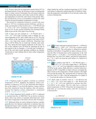
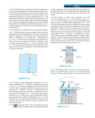
EXAMPLE 2–7 Convection and Insulation Boundary Conditions
Steam flows through a pipe shown in Fig. 2–34 at an average temperature
of T` 5 200°C. The inner and outer radii of the pipe are r1 5 8 cm and r2 5
8.5 cm, respectively, and the outer surface of the pipe is heavily insulated. If
the convection heat transfer coefficient on the inner surface of the pipe is h 5
65 W/m2
·K, express the boundary conditions on the inner and outer surfaces
of the pipe during transient periods.](https://image.slidesharecdn.com/25489135-230110133727-3d40a16a/85/25489135-pdf-110-320.jpg)
![88
HEAT CONDUCTION EQUATION
4 Radiation Boundary Condition
In some cases, such as those encountered in space and cryogenic applications,
a heat transfer surface is surrounded by an evacuated space and thus there is
no convection heat transfer between a surface and the surrounding medium. In
such cases, radiation becomes the only mechanism of heat transfer between
the surface under consideration and the surroundings. Using an energy bal-
ance, the radiation boundary condition on a surface can be expressed as
°
Heat conduction
at the surface in a
selected direction
¢ 5 °
Radiation exchange
at the surface in
the same direction
¢
For one-dimensional heat transfer in the x-direction in a plate of thickness L, the
radiation boundary conditions on both surfaces can be expressed as (Fig. 2–35)
2k
0T(0, t)
0x
5 e1s[T 4
surr, 1 2 T(0, t)4
] (2–52a)
and
2k
0T(L, t)
0x
5 e2s[T(L, t)4
2 T4
surr, 2] (2–52b)
where e1 and e2 are the emissivities of the boundary surfaces, s 5 5.67 3
1028
W/m2
·K4
is the Stefan–Boltzmann constant, and Tsurr, 1 and Tsurr, 2 are the
average temperatures of the surfaces surrounding the two sides of the plate,
respectively. Note that the temperatures in radiation calculations must be
expressed in K or R (not in °C or °F).
The radiation boundary condition involves the fourth power of temperature,
and thus it is a nonlinear condition. As a result, the application of this boundary
condition results in powers of the unknown coefficients, which makes it difficult
SOLUTION The flow of steam through an insulated pipe is considered.
The boundary conditions on the inner and outer surfaces of the pipe are to be
obtained.
Analysis During initial transient periods, heat transfer through the pipe mate-
rial predominantly is in the radial direction, and thus can be approximated as
being one-dimensional. Then the temperature within the pipe material changes
with the radial distance r and the time t. That is, T 5 T(r, t).
It is stated that heat transfer between the steam and the pipe at the inner
surface is by convection. Then taking the direction of heat transfer to be the
positive r direction, the boundary condition on that surface can be expressed as
2k
0T(r1, t)
0r
5 h[T` 2 T(r1)]
The pipe is said to be well insulated on the outside, and thus heat loss through
the outer surface of the pipe can be assumed to be negligible. Then the bound-
ary condition at the outer surface can be expressed as
0T(r2, t)
0r
5 0
Discussion Note that the temperature gradient must be zero on the outer sur-
face of the pipe at all times.
Insulation
r1
r2
h
T`
FIGURE 2–34
Schematic for Example 2–7.
0
Radiation Conduction
L x
Radiation
Conduction
1
Tsurr, 1
2
Tsurr, 2
e1 [Tsurr, 1 – T(0, t)4
] = –k
0T(0, t)
———
0x
4
s
=
–k
0T(L, t)
———
0x 2 [T(L, t)4
– Tsurr, 2]
4
s
e
e
e
FIGURE 2–35
Radiation boundary conditions on both
surfaces of a plane wall.](https://image.slidesharecdn.com/25489135-230110133727-3d40a16a/85/25489135-pdf-111-320.jpg)
![90
HEAT CONDUCTION EQUATION
SOLUTION The cooling of a hot spherical metal ball is considered. The initial
and boundary conditions are to be obtained.
Analysis The ball is initially at a uniform temperature and is cooled uniformly
from the entire outer surface. Therefore, this is a one-dimensional transient
heat transfer problem since the temperature within the ball changes with
the radial distance r and the time t. That is, T 5 T (r, t). Taking the moment
the ball is removed from the oven to be t 5 0, the initial condition can be
expressed as
T(r, 0) 5 Ti 5 600°F
The problem possesses symmetry about the midpoint (r 5 0) since the iso-
therms in this case are concentric spheres, and thus no heat is crossing the
midpoint of the ball. Then the boundary condition at the midpoint can be
expressed as
0T(0, t)
0r
5 0
The heat conducted to the outer surface of the ball is lost to the environment
by convection and radiation. Then taking the direction of heat transfer to be
the positive r direction, the boundary condition on the outer surface can be
expressed as
2k
0T(ro, t)
0r
5 h[T(ro) 2 T`] 1 es[T(ro)4
2 T4
surr]
Discussion All the quantities in the above relations are known except the tem-
peratures and their derivatives at r 5 0 and ro. Also, the radiation part of the
boundary condition is often ignored for simplicity by modifying the convection
heat transfer coefficient to account for the contribution of radiation. The convec-
tion coefficient h in that case becomes the combined heat transfer coefficient.
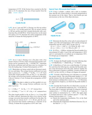
EXAMPLE 2–9 Combined Convection, Radiation, and Heat Flux
Consider the south wall of a house that is L 5 0.2 m thick. The outer surface
of the wall is exposed to solar radiation and has an absorptivity of a 5 0.5 for
solar energy. The interior of the house is maintained at T`1 5 20°C, while the
ambient air temperature outside remains at T`2 5 5°C. The sky, the ground,
and the surfaces of the surrounding structures at this location can be modeled
as a surface at an effective temperature of Tsky 5 255 K for radiation exchange
on the outer surface. The radiation exchange between the inner surface of
the wall and the surfaces of the walls, floor, and ceiling it faces is negligible.
The convection heat transfer coefficients on the inner and the outer surfaces
of the wall are h1 5 6 W/m2
·K and h2 5 25 W/m2
·K, respectively. The thermal
conductivity of the wall material is k 5 0.7 W/m·K, and the emissivity of the
outer surface is e2 5 0.9. Assuming the heat transfer through the wall to be
steady and one-dimensional, express the boundary conditions on the inner and
the outer surfaces of the wall.
SOLUTION The wall of a house subjected to solar radiation is considered.
The boundary conditions on the inner and outer surfaces of the wall are to be
obtained.](https://image.slidesharecdn.com/25489135-230110133727-3d40a16a/85/25489135-pdf-113-320.jpg)
![91
CHAPTER 2
Note that a heat transfer problem may involve different kinds of boundary
conditions on different surfaces. For example, a plate may be subject to heat
flux on one surface while losing or gaining heat by convection from the other
surface. Also, the two boundary conditions in a direction may be specified at
the same boundary, while no condition is imposed on the other boundary. For
example, specifying the temperature and heat flux at x 5 0 of a plate of thick-
ness L will result in a unique solution for the one-dimensional steady tempera-
ture distribution in the plate, including the value of temperature at the surface
x 5 L. Although not necessary, there is nothing wrong with specifying more
than two boundary conditions in a specified direction, provided that there is
no contradiction. The extra conditions in this case can be used to verify the
results.
2–5 ■
SOLUTION OF STEADY ONE-DIMENSIONAL
HEAT CONDUCTION PROBLEMS
So far we have derived the differential equations for heat conduction in
various coordinate systems and discussed the possible boundary conditions.
A heat conduction problem can be formulated by specifying the applicable
differential equation and a set of proper boundary conditions.
In this section we will solve a wide range of heat conduction problems
in rectangular, cylindrical, and spherical geometries. We will limit our at-
tention to problems that result in ordinary differential equations such as the
steady one-dimensional heat conduction problems. We will also assume con-
stant thermal conductivity, but will consider variable conductivity later in this
Analysis We take the direction normal to the wall surfaces as the x-axis with
the origin at the inner surface of the wall, as shown in Fig. 2–38. The heat
transfer through the wall is given to be steady and one-dimensional, and thus
the temperature depends on x only and not on time. That is, T 5 T(x).
The boundary condition on the inner surface of the wall at x 5 0 is a typical
convection condition since it does not involve any radiation or specified heat
flux. Taking the direction of heat transfer to be the positive x-direction, the
boundary condition on the inner surface can be expressed as
2k
dT(0)
dx
5 h1[T`1 2 T(0)]
The boundary condition on the outer surface at x 5 0 is quite general as it
involves conduction, convection, radiation, and specified heat flux. Again tak-
ing the direction of heat transfer to be the positive x-direction, the boundary
condition on the outer surface can be expressed as
2k
dT(L)
dx
5 h2[T(L) 2 T`2] 1 e2s[T(L)4
2 T4
sky] 2 aq
·
solar
where q
·
solar is the incident solar heat flux.
Discussion Assuming the opposite direction for heat transfer would give the
same result multiplied by 21, which is equivalent to the relation here. All the
quantities in these relations are known except the temperatures and their de-
rivatives at the two boundaries.
Conduction
Conduction
Convection
Convection
Radiation
Solar
Tsky
South
wall
Inner
surface
0
L x
h1
T`1
h2
T`2
Sun
Outer
surface
FIGURE 2–38
Schematic for Example 2–9.](https://image.slidesharecdn.com/25489135-230110133727-3d40a16a/85/25489135-pdf-114-320.jpg)
![96
HEAT CONDUCTION EQUATION
Discussion The last solution represents a family of straight lines whose slope
is 2q
·
0/k. Physically, this problem corresponds to requiring the rate of heat
supplied to the wall at x 5 0 be equal to the rate of heat removal from the
other side of the wall at x 5 L. But this is a consequence of the heat conduc-
tion through the wall being steady, and thus the second boundary condition
does not provide any new information. So it is not surprising that the solution
of this problem is not unique. The three cases discussed above are summarized
in Fig. 2–44.
T˝(x) = 0
T(x) = C1x + C2
x + T0
T(x) = –
–kT′(0) = q0 q0
k
T′(0) = T0
Differential equation:
General solution:
(a) Unique solution:
· ·
x + C2
T(x) = –
q0
k
·
T(x) = None
Arbitrary
–kT′(0) = q0
–kT′(L) = qL
(b) No solution:
·
·
·
–kT′(0) = q0
–kT′(L) = q0
(c) Multiple solutions:
·
↑
FIGURE 2–44
A boundary-value problem may have
a unique solution, infinitely many
solutions, or no solutions at all.
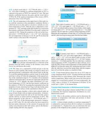
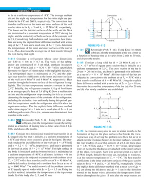
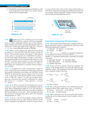
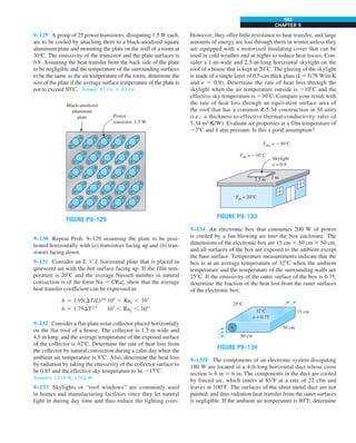
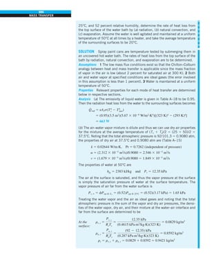
EXAMPLE 2–12 Heat Conduction in the Base Plate of an Iron
Consider the base plate of a 1200-W household iron that has a thickness of
L 5 0.5 cm, base area of A 5 300 cm2
, and thermal conductivity of k 5
15 W/m·K. The inner surface of the base plate is subjected to uniform heat flux
generated by the resistance heaters inside, and the outer surface loses heat to
the surroundings at T` 5 20°C by convection, as shown in Fig. 2–45. Taking the
convection heat transfer coefficient to be h 5 80 W/m2
·K and disregarding heat
loss by radiation, obtain an expression for the variation of temperature in the
base plate, and evaluate the temperatures at the inner and the outer surfaces.
SOLUTION The base plate of an iron is considered. The variation of tempera-
ture in the plate and the surface temperatures are to be determined.
Assumptions 1 Heat transfer is steady since there is no change with time.
2 Heat transfer is one-dimensional since the surface area of the base plate is
large relative to its thickness, and the thermal conditions on both sides are
uniform. 3 Thermal conductivity is constant. 4 There is no heat generation in
the medium. 5 Heat transfer by radiation is negligible. 6 The upper part of the
iron is well insulated so that the entire heat generated in the resistance wires
is transferred to the base plate through its inner surface.
Properties The thermal conductivity is given to be k 5 15 W/m·K.
Analysis The inner surface of the base plate is subjected to uniform heat flux
at a rate of
q
·
0 5
Q
#
0
Abase
5
1200 W
0.03 m2
5 40,000 W/m2
The outer side of the plate is subjected to the convection condition. Taking the
direction normal to the surface of the wall as the x-direction with its origin on
the inner surface, the differential equation for this problem can be expressed
as (Fig. 2–46)
d2
T
dx2
5 0
with the boundary conditions
2 k
dT(0)
dx
5 q
·
0 5 40,000 W/m2
2 k
dT(L)
dx
5 h[T(L) 2 T`]
x
h
L
Base plate
T` = 20°C
300 cm2
Insulation
Resistance heater
1200 W
FIGURE 2–45
Schematic for Example 2–12.](https://image.slidesharecdn.com/25489135-230110133727-3d40a16a/85/25489135-pdf-119-320.jpg)
![97
CHAPTER 2
The general solution of the differential equation is again obtained by two suc-
cessive integrations to be
dT
dx
5 C1
and
T(x) 5 C1x 1 C2 (a)
where C1 and C2 are arbitrary constants. Applying the first boundary condition,
2k
dT(0)
dx
5 q
·
0 S 2kC1 5 q·
0 S C1 5 2
q
#
0
k
Noting that dT/dx 5 C1 and T(L) 5 C1L 1 C2, the application of the second
boundary condition gives
2k
dT(L)
dx
5 h[T(L) 2 T`] S 2kC1 5 h[(C1L 1 C2) 2 T`]
Substituting C1 5 2q
·
0/k and solving for C2, we obtain
C2 5 T` 1
q
#
0
h
1
q
#
0
k
L
Now substituting C1 and C2 into the general solution (a) gives
T(x) 5 T` 1 q·
0a
L 2 x
k
1
1
h
b (b)
which is the solution for the variation of the temperature in the plate. The
temperatures at the inner and outer surfaces of the plate are determined by
substituting x 5 0 and x 5 L, respectively, into the relation (b):
T(0) 5 T` 1 q
·
0a
L
k
1
1
h
b
5 20°C 1 (40,000 W/m2
)a
0.005 m
15 W/m·K
1
1
80 W/m2
·K
b 5 533°C
and
T(L) 5 T` 1 q
·
0a0 1
1
h
b 5 20°C 1
40,000 W/m2
80 W/m2
·K
5 520°C
Discussion Note that the temperature of the inner surface of the base plate
is 13°C higher than the temperature of the outer surface when steady operat-
ing conditions are reached. Also note that this heat transfer analysis enables
us to calculate the temperatures of surfaces that we cannot even reach. This
example demonstrates how the heat flux and convection boundary conditions
are applied to heat transfer problems.
0
Heat flux Conduction
Base plate
L x
Convection
h
T`
Conduction
q0 = –k
dT(0)
–——
dx
·
–k = h[T(L) – T`]
dT(L)
–——
dx
FIGURE 2–46
The boundary conditions on the
base plate of the iron discussed
in Example 2–12.](https://image.slidesharecdn.com/25489135-230110133727-3d40a16a/85/25489135-pdf-120-320.jpg)
![98
HEAT CONDUCTION EQUATION
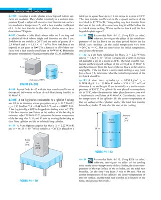
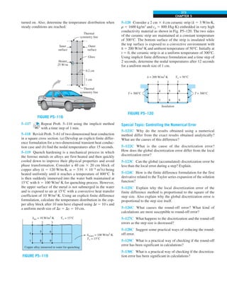
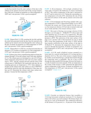
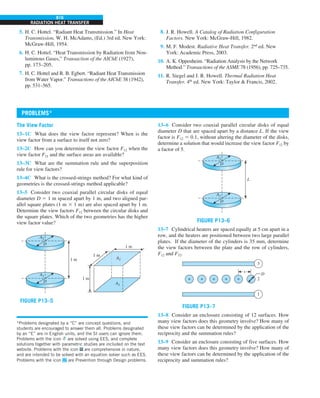
EXAMPLE 2–13 Thermal Burn Prevention in Metal
Processing Plant
In metal processing plants, workers often operate near hot metal surfaces.
Exposed hot surfaces are hazards that can potentially cause thermal burns on
human skin tissue. Metallic surface with a temperature above 70°C is con-
sidered extremely hot. Damage to skin tissue can occur instantaneously upon
contact with metallic surface at that temperature. In a plant that processes
metal plates, a plate is conveyed through a series of fans to cool its surface
in an ambient temperature of 30°C, as shown in Figure 2-47. The plate is
25 mm thick and has a thermal conductivity of 13.5 W/m∙K. Temperature at
the bottom surface of the plate is monitored by an infrared (IR) thermometer.
Obtain an expression for the variation of temperature in the metal plate. The
IR thermometer measures the bottom surface of the plate to be 60°C. Deter-
mine the minimum value of the convection heat transfer coefficient necessary
to keep the top surface below 47°C to avoid instantaneous thermal burn upon
accidental contact of hot metal surface with skin tissue.
SOLUTION In this example, the concepts of Prevention through Design (PtD)
are applied in conjunction with the solution of steady one-dimensional heat
conduction problem. The top surface of the plate is cooled by convection, and
temperature at the bottom surface is measured by an IR thermometer. The
variation of temperature in the metal plate and the convection heat transfer
coefficient necessary to keep the top surface below 47°C are to be determined.
Assumptions 1 Heat conduction is steady and one-dimensional. 2 Thermal
conductivity is constant. 3 There is no heat generation in the plate. 4 The bot-
tom surface at x 5 0 is at constant temperature while the top surface at x 5 L
is subjected to convection.
Properties The thermal conductivity of the metal plate is given to be k 5
13.5 W/m∙K.
Analysis Taking the direction normal to the surface of the wall to be the x
direction with x 5 0 at the lower surface, the mathematical formulation can
be expressed as
d2
T
dx2
5 0
with boundary conditions
T(0) 5 T0
2k
dT(L)
dx
5 h[T(L) 2 Tq]
Integrating the differential equation twice with respect to x yields
dT
dx
5 C1
T(x) 5 C1x 1 C2
where C1 and C2 are arbitrary constants. Applying the first boundary condition
yields
T(0) 5 C1 3 0 1 C2 5 T0 S C2 5 T0
FIGURE 2–47
Schematic for Example 2–13.
h, T`
Metal plate k
TL
T0
L
0
IR
x](https://image.slidesharecdn.com/25489135-230110133727-3d40a16a/85/25489135-pdf-121-320.jpg)
![99
CHAPTER 2
The application of the second boundary condition gives
2k
dT(L)
dx
5 h[T(L) 2 Tq] S 2kC1 5 h(C1L 1 C2 2 Tq)
Solving for C1 yields
C1 5
h(Tq 2 C2)
k 1 hL
5
Tq 2 T0
(k/h) 1 L
Now substituting C1 and C2 into the general solution, the variation of tempera-
ture becomes
T(x) 5
Tq 2 T0
(k/h) 1 L
x 1 T0
The minimum convection heat transfer coefficient necessary to maintain the
top surface below 47°C can be determined from the variation of temperature:
T(L) 5 TL 5
Tq 2 T0
(k/h) 1 L
L 1 T0
Solving for h gives
h 5
k
L
TL 2 T0
Tq 2 TL
5 a
13.5 W/m·K
0.025 m
b
(47 2 60)8C
(30 2 47)8C
5 413 W/m2
·K
Discussion To keep the top surface of the metal plate below 47°C, the con-
vection heat transfer coefficient should be greater than 413 W/m2
∙K. A con-
vection heat transfer coefficient value of 413 W/m2
∙K is very high for forced
convection of gases. The typical values for forced convection of gases are
25–250 W/m2
∙K (see Table 1-5 in Chapter 1). To protect workers from thermal
burn, appropriate apparel should be worn when operating in an area where hot
surfaces are present.
0
Plane wall
L x
e
Conduction
Space
R
a
d
i
a
t
i
o
n
S
o
l
a
r
Sun
T1
a
FIGURE 2–48
Schematic for Example 2–14.
EXAMPLE 2–14 Heat Conduction in a Solar Heated Wall
Consider a large plane wall of thickness L 5 0.06 m and thermal conductivity
k 5 1.2 W/m·K in space. The wall is covered with white porcelain tiles that have
an emissivity of e 5 0.85 and a solar absorptivity of a 5 0.26, as shown in
Fig. 2–48. The inner surface of the wall is maintained at T1 5 300 K at all times,
while the outer surface is exposed to solar radiation that is incident at a rate of
q
·
solar 5 800 W/m2
. The outer surface is also losing heat by radiation to deep space
at 0 K. Determine the temperature of the outer surface of the wall and the rate
of heat transfer through the wall when steady operating conditions are reached.
What would your response be if no solar radiation was incident on the surface?
SOLUTION A plane wall in space is subjected to specified temperature on
one side and solar radiation on the other side. The outer surface temperature
and the rate of heat transfer are to be determined.
Assumptions 1 Heat transfer is steady since there is no change with time.
2 Heat transfer is one-dimensional since the wall is large relative to its
thickness, and the thermal conditions on both sides are uniform. 3 Thermal
conductivity is constant. 4 There is no heat generation.](https://image.slidesharecdn.com/25489135-230110133727-3d40a16a/85/25489135-pdf-122-320.jpg)
![100
HEAT CONDUCTION EQUATION
Properties The thermal conductivity is given to be k 5 1.2 W/m·K.
Analysis Taking the direction normal to the surface of the wall as the
x-direction with its origin on the inner surface, the differential equation for this
problem can be expressed as
d2
T
dx2
5 0
with boundary conditions
T(0) 5 T1 5 300 K
2k
dT(L)
dx
5 es[T(L)4
2 T4
space] 2 aq
·
solar
where Tspace 5 0. The general solution of the differential equation is again
obtained by two successive integrations to be
T(x) 5 C1x 1 C2 (a)
where C1 and C2 are arbitrary constants. Applying the first boundary condition
yields
T(0) 5 C1 3 0 1 C2 S C2 5 T1
Noting that dT/dx 5 C1 and T(L) 5 C1L 1 C2 5 C1L 1 T1, the application of
the second boundary conditions gives
2k
dT(L)
dx
5 esT(L)4
2 aq
·
solar S 2kC1 5 es(C1L 1 T1)4
2 aq
·
solar
Although C1 is the only unknown in this equation, we cannot get an explicit
expression for it because the equation is nonlinear, and thus we cannot get a
closed-form expression for the temperature distribution. This should explain
why we do our best to avoid nonlinearities in the analysis, such as those as-
sociated with radiation.
Let us back up a little and denote the outer surface temperature by T(L) 5 TL
instead of T(L) 5 C1L 1 T1. The application of the second boundary condition
in this case gives
2k
dT(L)
dx
5 esT(L)4
2 aq
·
solar S 2kC1 5 esT4
L 2 aq
·
solar
Solving for C1 gives
C1 5
aq
#
solar 2 esT4
L
k
(b)
Now substituting C1 and C2 into the general solution (a), we obtain
T(x) 5
aq
#
solar 2 esT4
L
k
x 1 T1 (c)
which is the solution for the variation of the temperature in the wall in terms of
the unknown outer surface temperature TL. At x 5 L it becomes
TL 5
aq
#
solar 2 esT4
L
k
L 1 T1 (d )](https://image.slidesharecdn.com/25489135-230110133727-3d40a16a/85/25489135-pdf-123-320.jpg)

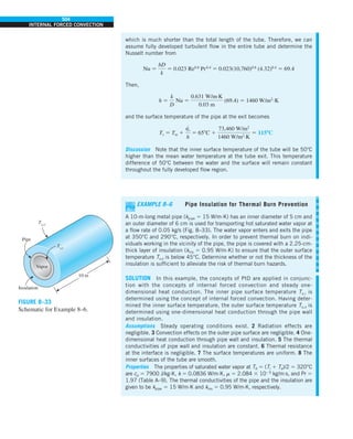
![114
HEAT CONDUCTION EQUATION
Bronze
plate
k(T) = k0(1 + bT)
T2 = 400 K
T1 = 600 K
Q
·
L
FIGURE 2–66
Schematic for Example 2–22.
where A is the heat conduction area of the wall and
kavg 5 k(Tavg) 5 k0a1 1 b
T2 1 T1
2
b
is the average thermal conductivity (Eq. 2–80).
(b) To determine the temperature distribution in the wall, we begin with Fourier’s
law of heat conduction, expressed as
Q
·
5 2k(T) A
dT
dx
where the rate of conduction heat transfer Q
·
and the area A are constant.
Separating variables and integrating from x 5 0 where T (0) 5 T1 to any x
where T(x) 5 T, we get
#
x
0
Q
·
dx 5 2A #
T
T1
k(T)dT
Substituting k(T) 5 k0(1 1 bT ) and performing the integrations we obtain
Q
·
x 5 2Ak0[(T 2 T1) 1 b(T 2
2 T2
1)/2]
Substituting the Q
·
expression from part (a) and rearranging give
T2
1
2
b
T 1
2kavg
bk0
x
L
(T1 2 T2) 2 T2
1 2
2
b
T1 5 0
which is a quadratic equation in the unknown temperature T. Using the qua-
dratic formula, the temperature distribution T(x) in the wall is determined to be
T(x) 5 2
1
b
6
Å
1
b2
2
2kavg
bk0
x
L
(T1 2 T2) 1 T2
1 1
2
b
T1
Discussion The proper sign of the square root term (1 or 2) is determined
from the requirement that the temperature at any point within the medium
must remain between T1 and T2. This result explains why the temperature
distribution in a plane wall is no longer a straight line when the thermal con-
ductivity varies with temperature.
EXAMPLE 2–22 Heat Conduction through a Wall with k(T )
Consider a 2-m-high and 0.7-m-wide bronze plate whose thickness is 0.1 m.
One side of the plate is maintained at a constant temperature of 600 K while
the other side is maintained at 400 K, as shown in Fig. 2–66. The thermal
conductivity of the bronze plate can be assumed to vary linearly in that tem-
perature range as k(T) 5 k0(1 1 bT) where k0 5 38 W/m·K and b 5 9.21 3
1024
K21
. Disregarding the edge effects and assuming steady one-dimensional
heat transfer, determine the rate of heat conduction through the plate.
SOLUTION A plate with variable conductivity is subjected to specified tem-
peratures on both sides. The rate of heat transfer is to be determined.
Assumptions 1 Heat transfer is given to be steady and one-dimensional.
2 Thermal conductivity varies linearly. 3 There is no heat generation.](https://image.slidesharecdn.com/25489135-230110133727-3d40a16a/85/25489135-pdf-137-320.jpg)
![CHAPTER 2
121
In this chapter we have studied the heat conduction equation and
its solutions. Heat conduction in a medium is said to be steady
when the temperature does not vary with time and unsteady or
transient when it does. Heat conduction in a medium is said
to be one-dimensional when conduction is significant in one
dimension only and negligible in the other two dimensions. It is
said to be two-dimensional when conduction in the third dimen-
sion is negligible and three-dimensional when conduction in all
dimensions is significant. In heat transfer analysis, the conver-
sion of electrical, chemical, or nuclear energy into heat (or ther-
mal) energy is characterized as heat generation.
The heat conduction equation can be derived by performing
an energy balance on a differential volume element. The one-
dimensional heat conduction equation in rectangular, cylindri-
cal, and spherical coordinate systems for the case of constant
thermal conductivities are expressed as
02
T
0x2
1
e
#
gen
k
5
1
a
0T
0t
1
r
0
0r
ar
0T
0r
b 1
e
#
gen
k
5
1
a
0T
0t
1
r2
0
0r
ar2
0T
0r
b 1
e
#
gen
k
5
1
a
0T
0t
where the property a 5 k/rc is the thermal diffusivity of the
material.
The solution of a heat conduction problem depends on the
conditions at the surfaces, and the mathematical expressions
for the thermal conditions at the boundaries are called the
boundary conditions. The solution of transient heat conduction
problems also depends on the condition of the medium at the
beginning of the heat conduction process. Such a condition,
which is usually specified at time t 5 0, is called the initial
condition, which is a mathematical expression for the tem-
perature distribution of the medium initially. Complete math-
ematical description of a heat conduction problem requires
the specification of two boundary conditions for each dimen-
sion along which heat conduction is significant, and an initial
condition when the problem is transient. The most common
boundary conditions are the specified temperature, specified
heat flux, convection, and radiation boundary conditions. A
boundary surface, in general, may involve specified heat flux,
convection, and radiation at the same time.
For steady one-dimensional heat transfer through a plate of
thickness L, the various types of boundary conditions at the
surfaces at x 5 0 and x 5 L can be expressed as
Specified temperature:
T(0) 5 T1 and T(L) 5 T2
where T1 and T2 are the specified temperatures at surfaces at
x 5 0 and x 5 L.
Specified heat flux:
2k
dT(0)
dx
5 q
·
0 and 2k
dT(L)
dx
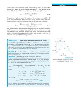
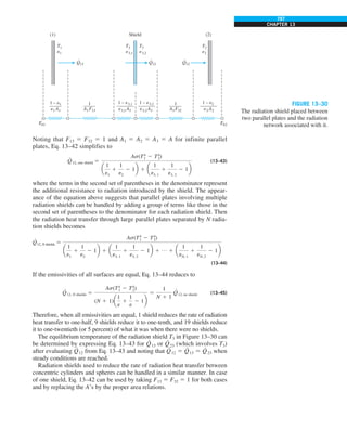
5 q
·
L
where q
·
0 and q
·
L are the specified heat fluxes at surfaces at
x 5 0 and x 5 L.
Insulation or thermal symmetry:
dT(0)
dx
5 0 and
dT(L)
dx
5 0
Convection:
2k
dT(0)
dx
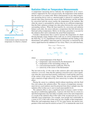
5 h1[T`1 2 T(0)] and 2k
dT(L)
dx
5 h2[T(L) 2 T`2]
where h1 and h2 are the convection heat transfer coefficients
and T`1 and T`2 are the temperatures of the surrounding medi-
ums on the two sides of the plate.
Radiation:
2k
dT(0)
dx
5 e1s[T4
surr, 1 2 T(0)4
] and
2k
dT(L)
dx
5 e2s[T(L)4
2 T4
surr, 2]
where e1 and e2 are the emissivities of the boundary surfaces,
s 5 5.67 3 1028
W/m2
·K4
is the Stefan–Boltzmann constant,
and Tsurr, 1 and Tsurr, 2 are the average temperatures of the sur-
faces surrounding the two sides of the plate. In radiation calcu-
lations, the temperatures must be in K or R.
Interface of two bodies A and B in perfect contact at x 5 x0:
TA (x0) 5 TB (x0) and 2kA
dTA (x0)
dx
5 2kB
dTB (x0)
dx
where kA and kB are the thermal conductivities of the layers
A and B.
Heat generation is usually expressed per unit volume of the
medium and is denoted by e
·
gen, whose unit is W/m3
. Under
steady conditions, the surface temperature Ts of a plane wall
of thickness 2L, a cylinder of outer radius ro, and a sphere
of radius ro in which heat is generated at a constant rate of
SUMMARY](https://image.slidesharecdn.com/25489135-230110133727-3d40a16a/85/25489135-pdf-144-320.jpg)
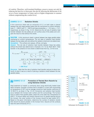
![140
HEAT CONDUCTION EQUATION
2–158 Consider a large plane wall of thickness L, thermal
conductivity k, and surface area A. The left surface of the wall
is exposed to the ambient air at T` with a heat transfer coeffi-
cient of h while the right surface is insulated. The variation of
temperature in the wall for steady one-dimensional heat con-
duction with no heat generation is
(a) T(x) 5
h(L 2 x)
k
T`
(b) T(x) 5
k
h(x 1 0.5L)
T`
(c) T(x) 5 a1 2
xh
k
b T`
(d) T(x) 5 (L 2 x) T`
(e) T(x) 5 T`
2–159 A solar heat flux q
·
s is incident on a sidewalk whose ther-
mal conductivity is k, solar absorptivity is as, and convective
heat transfer coefficient is h. Taking the positive x direction to
be towards the sky and disregarding radiation exchange with the
surroundings surfaces, the correct boundary condition for this
sidewalk surface is
(a) 2k
dT
dx
5 as q
.
s (b) 2k
dT
dx
5 h(T 2 T`)
(c) 2k
dT
dx
5 h(T 2 T`) 2 as q
.
s (d) h(T 2 T`) 5 as q
.
s
(e) None of them
2–160 A plane wall of thickness L is subjected to convection
at both surfaces with ambient temperature T`1 and heat transfer
coefficient h1 at inner surface, and corresponding T`2 and h2
values at the outer surface. Taking the positive direction of x
to be from the inner surface to the outer surface, the correct
expression for the convection boundary condition is
(a) k
dT(0)
dx
5 h1[T(0) 2 T`1)]
(b) k
dT(L)
dx
5 h2[T(L) 2 T`2)]
(c) 2k
dT(0)
dx
5 h1[T`1 2 T`2)]
(d) 2k
dT(L)
dx
5 h2[T`1 2 T`2)]
(e) None of them
2–161 Consider steady one-dimensional heat conduction
through a plane wall, a cylindrical shell, and a spherical shell
of uniform thickness with constant thermophysical properties
and no thermal energy generation. The geometry in which the
variation of temperature in the direction of heat transfer will
be linear is
(a) plane wall (b) cylindrical shell (c) spherical shell
(d) all of them (e) none of them
2–162 The conduction equation boundary condition for
an adiabatic surface with direction n being normal to the
surface is
(a) T 5 0 (b) dT/dn 5 0 (c) d2
T/dn2
5 0
(d) d3
T/dn3
5 0 (e) 2kdT/dn 5 1
2–163 The variation of temperature in a plane wall is deter-
mined to be T(x) 5 52x 1 25 where x is in m and T is in °C. If the
temperature at one surface is 38°C, the thickness of the wall is
(a) 0.10 m (b) 0.20 m (c) 0.25 m
(d) 0.40 m (e) 0.50 m
2–164 The variation of temperature in a plane wall is deter-
mined to be T(x) 5 110260x where x is in m and T is in °C. If
the thickness of the wall is 0.75 m, the temperature difference
between the inner and outer surfaces of the wall is
(a) 30°C (b) 45°C (c) 60°C (d) 75°C (e) 84°C
2–165 The temperatures at the inner and outer surfaces of a
15-cm-thick plane wall are measured to be 40°C and 28°C, re-
spectively. The expression for steady, one-dimensional varia-
tion of temperature in the wall is
(a) T(x) 5 28x 1 40 (b) T(x) 5 240x 1 28
(c) T(x) 5 40x 1 28 (d) T(x) 5 280x 1 40
(e) T(x) 5 40x 2 80
2–166 The thermal conductivity of a solid depends upon the
solid’s temperature as k 5 aT 1 b where a and b are constants.
The temperature in a planar layer of this solid as it conducts
heat is given by
(a) aT 1 b 5 x 1 C2 (b) aT 1 b 5 C1x2
1 C2
(c) aT2
1 bT 5 C1x 1 C2 (d) aT2
1 bT 5 C1x2
1 C2
(e) None of them
2–167 Hot water flows through a PVC (k 5 0.092 W/m·K)
pipe whose inner diameter is 2 cm and outer diameter is
2.5 cm. The temperature of the interior surface of this pipe is
50°C and the temperature of the exterior surface is 20°C. The
rate of heat transfer per unit of pipe length is
(a) 77.7 W/m (b) 89.5 W/m (c) 98.0 W/m
(d) 112 W/m (e) 168 W/m
2–168 Heat is generated in a long 0.3-cm-diameter cylindri-
cal electric heater at a rate of 180 W/cm3
. The heat flux at the
surface of the heater in steady operation is
(a) 12.7 W/cm2
(b) 13.5 W/cm2
(c) 64.7 W/cm2
(d) 180 W/cm2
(e) 191 W/cm2
2–169 Heat is generated uniformly in a 4-cm-diameter,
12-cm-long solid bar (k 5 2.4 W/m·K). The temperatures at
the center and at the surface of the bar are measured to be
210°C and 45°C, respectively. The rate of heat generation
within the bar is
(a) 597 W (b) 760 W (c) 826 W
(d) 928 W (e) 1020 W
2–170 Heat is generated in a 10-cm-diameter spherical
radioactive material whose thermal conductivity is 25 W/m·K](https://image.slidesharecdn.com/25489135-230110133727-3d40a16a/85/25489135-pdf-163-320.jpg)
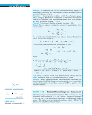
![151
CHAPTER 3
Assumptions 1 Heat transfer through the window is steady since the surface
temperatures remain constant at the specified values. 2 Heat transfer through
the wall is one-dimensional since any significant temperature gradients exist
in the direction from the indoors to the outdoors. 3 Thermal conductivity is
constant.
Properties The thermal conductivity is given to be k 5 0.78 W/m·K.
Analysis This problem involves conduction through the glass window and con-
vection at its surfaces, and can best be handled by making use of the thermal
resistance concept and drawing the thermal resistance network, as shown in
Fig. 3–12. Noting that the area of the window is A 5 0.8 m 3 1.5 m 5
1.2 m2
, the individual resistances are evaluated from their definitions to be
Ri 5 Rconv, 1 5
1
h1 A
5
1
(10 W/m2
·K)(1.2 m2
)
5 0.083338C/W
Rglass 5
L
kA
5
0.008 m
(0.78 W/m·K)(1.2 m2
)
5 0.008558C/W
Ro 5 Rconv, 2 5
1
h2 A
5
1
(40 W/m2
·K)(1.2 m2
)
5 0.020838C/W
Noting that all three resistances are in series, the total resistance is
Rtotal 5 Rconv, 1 1 Rglass 1 Rconv, 2 5 0.08333 1 0.00855 1 0.02083
5 0.11278C/W
Then the steady rate of heat transfer through the window becomes
Q
#
5
Tq1 2 Tq2
Rtotal
5
[20 2 (210)]8C
0.11278C/ W
5 266 W
Knowing the rate of heat transfer, the inner surface temperature of the window
glass can be determined from
Q
#
5
Tq1 2 T1
Rconv, 1
h T1 5 T`1 2 Q
#
Rconv, 1
5 208C 2 (266 W)(0.083338C/W)
5 22.28C
Discussion Note that the inner surface temperature of the window glass is
22.2°C even though the temperature of the air in the room is maintained at
20°C. Such low surface temperatures are highly undesirable since they cause
the formation of fog or even frost on the inner surfaces of the glass when the
humidity in the room is high.
T2
Rglass Ro
L = 8 mm
Ri
T1 T2
T1
h1 = 10 W/m2
·K h2 = 40 W/m2
·K
Glass
20°C
–10°C
T`1 T`2
FIGURE 3–12
Schematic for Example 3–2.
EXAMPLE 3–3 Heat Loss through Double-Pane Windows
Consider a 0.8-m-high and 1.5-m-wide double-pane window consisting of two
4-mm-thick layers of glass (k 5 0.78 W/m·K) separated by a 10-mm-wide
stagnant air space (k 5 0.026 W/m·K). Determine the steady rate of heat](https://image.slidesharecdn.com/25489135-230110133727-3d40a16a/85/25489135-pdf-174-320.jpg)
![152
STEADY HEAT CONDUCTION
transfer through this double-pane window and the temperature of its inner sur-
face for a day during which the room is maintained at 20°C while the tempera-
ture of the outdoors is 210°C. Take the convection heat transfer coefficients
on the inner and outer surfaces of the window to be h1 5 10 W/m2
·K and
h2 5 40 W/m2
·K, which includes the effects of radiation.
SOLUTION A double-pane window is considered. The rate of heat transfer
through the window and the inner surface temperature are to be determined.
Analysis This example problem is identical to the previous one except that
the single 8-mm-thick window glass is replaced by two 4-mm-thick glasses
that enclose a 10-mm-wide stagnant air space. Therefore, the thermal resis-
tance network of this problem involves two additional conduction resistances
corresponding to the two additional layers, as shown in Fig. 3–13. Noting that
the area of the window is again A 5 0.8 m 3 1.5 m 5 1.2 m2
, the individual
resistances are evaluated from their definitions to be
Ri 5 Rconv, 1 5
1
h1 A
5
1
(10 W/m2
·K)(1.2 m2
)
5 0.083338C/W
R1 5 R3 5 Rglass 5
L1
k1 A
5
0.004 m
(0.78 W/m·K)(1.2 m2
)
5 0.004278C/W
R2 5 Rair 5
L2
k2 A
5
0.01 m
(0.026 W/m·K)(1.2 m2
)
5 0.32058C/W
Ro 5 Rconv, 2 5
1
h2 A
5
1
(40 W/m2
·K)(1.2 m2
)
5 0.020838C/W
Noting that all three resistances are in series, the total resistance is
Rtotal 5 Rconv, 1 1 Rglass, 1 1 Rair 1 Rglass, 2 1 Rconv, 2
5 0.08333 1 0.00427 1 0.3205 1 0.00427 1 0.02083
5 0.43328C/W
Then the steady rate of heat transfer through the window becomes
Q
#
5
Tq1 2 Tq2
Rtotal
5
[20 2 (210)]8C
0.43328C/ W
5 69.2 W
which is about one-fourth of the result obtained in the previous example. This
explains the popularity of the double- and even triple-pane windows in cold
climates. The drastic reduction in the heat transfer rate in this case is due to
the large thermal resistance of the air layer between the glasses.
The inner surface temperature of the window in this case will be
T1 5 T`1 2 Q
#
Rconv, 1 5 208C 2 (69.2 W)(0.083338C/W) 5 14.28C
which is considerably higher than the 22.2°C obtained in the previous
example. Therefore, a double-pane window will rarely get fogged. A double-
pane window will also reduce the heat gain in summer, and thus reduce the air-
conditioning costs.
T1
T2
T3
R1
Ri R3
R2
T4
10 mm
20°C
Air
Glass Glass
–10°C
4 mm 4 mm
Ro T`2
T`1
FIGURE 3–13
Schematic for Example 3–3.](https://image.slidesharecdn.com/25489135-230110133727-3d40a16a/85/25489135-pdf-175-320.jpg)
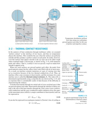
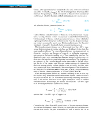
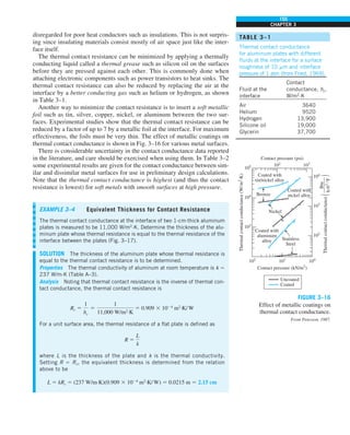
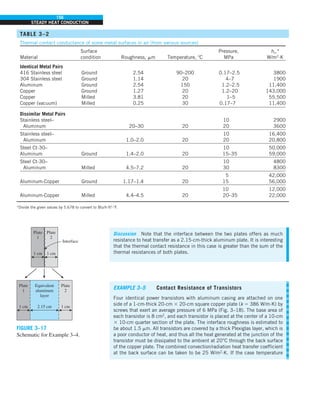
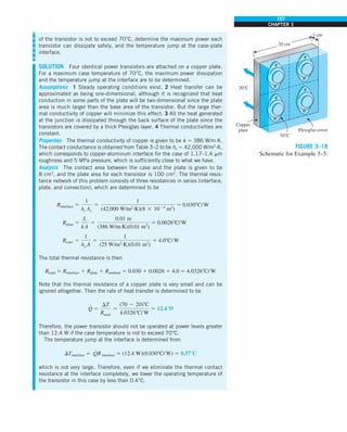
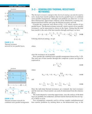
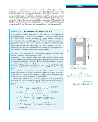
![160
STEADY HEAT CONDUCTION
R4 5 Rbrick 5
L
k A
5
0.16 m
(0.72 W/m·K)(0.22 3 1 m2
)
5 1.018C/W
Ro 5 Rconv, 2 5
1
h2 A
5
1
(25 W/m2
·K)(0.25 3 1 m2
)
5 0.168C/W
The three resistances R3, R4, and R5 in the middle are parallel, and their equiv-
alent resistance is determined from
1
Rmid
5
1
R3
1
1
R4
1
1
R5
5
1
48.48
1
1
1.01
1
1
48.48
5 1.03 W/8C
which gives
Rmid 5 0.978C/W
Now all the resistances are in series, and the total resistance is
Rtotal 5 Ri 1 R1 1 R2 1 Rmid 1 R6 1 Ro
5 0.40 1 4.62 1 0.36 1 0.97 1 0.36 1 0.16
5 6.878C/W
Then the steady rate of heat transfer through the wall becomes
Q
#
5
Tq1 2 Tq2
Rtotal
5
[20 2 (210)]8C
6.878C/ W
5 4.37 W (per 0.25 m2
surface area)
or 4.37/0.25 5 17.5 W per m2
area. The total area of the wall is A 5 3 m 3
5 m 5 15 m2
. Then the rate of heat transfer through the entire wall becomes
Q
#
total 5 (17.5 W/m2
)(15 m2
) 5 263 W
Of course, this result is approximate, since we assumed the temperature within
the wall to vary in one direction only and ignored any temperature change (and
thus heat transfer) in the other two directions.
Discussion In the above solution, we assumed the temperature at any cross
section of the wall normal to the x-direction to be isothermal. We could also
solve this problem by going to the other extreme and assuming the surfaces par-
allel to the x-direction to be adiabatic. The thermal resistance network in this
case will be as shown in Fig. 3–22. By following the approach outlined above,
the total thermal resistance in this case is determined to be Rtotal 5 6.97°C/W,
which is very close to the value 6.85°C/W obtained before. Thus either
approach gives roughly the same result in this case. This example demon-
strates that either approach can be used in practice to obtain satisfactory
results.
x
Ro
T`2
Ri
T`1
Adiabatic
lines
FIGURE 3–22
Alternative thermal resistance
network for Example 3–6 for the
case of surfaces parallel to the
primary direction of heat
transfer being adiabatic.](https://image.slidesharecdn.com/25489135-230110133727-3d40a16a/85/25489135-pdf-183-320.jpg)
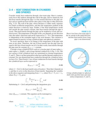
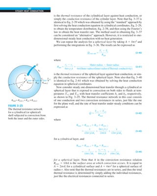
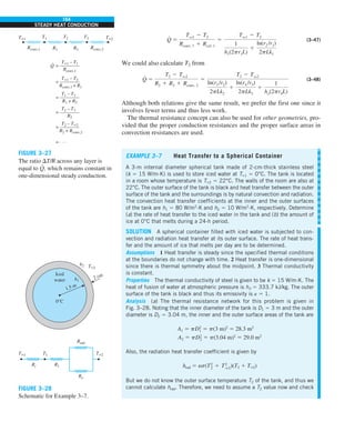
![165
CHAPTER 3
the accuracy of this assumption later. We will repeat the calculations if neces-
sary using a revised value for T2.
We note that T2 must be between 0°C and 22°C, but it must be closer to
0°C, since the heat transfer coefficient inside the tank is much larger. Taking
T2 5 5°C 5 278 K, the radiation heat transfer coefficient is determined to be
hrad 5 (1)(5.67 3 1028
W/m2
·K4
)[(295 K)2
1 (278 K)2
][(295 1 278) K]
5 5.34 W/m2
·K 5 5.34 W/m2
·8C
Then the individual thermal resistances become
Ri 5 Rconv, 1 5
1
h1 A1
5
1
(80 W/m2
·K)(28.3 m2
)
5 0.0004428C/W
R1 5 Rsphere 5
r2 2 r1
4pkr1r2
5
(1.52 2 1.50) m
4p (15 W/m·K)(1.52 m)(1.50 m)
5 0.0000478C/W
Ro 5 Rconv, 2 5
1
h2 A2
5
1
(10 W/m2
·K)(29.0 m2
)
5 0.003458C/W
Rrad 5
1
hrad A2
5
1
(5.34 W/m2
·K)(29.0 m2
)
5 0.006468C/W
The two parallel resistances Ro and Rrad can be replaced by an equivalent
resistance Requiv determined from
1
Requiv
5
1
Ro
1
1
Rrad
5
1
0.00345
1
1
0.00646
5 444.7 W/8C
which gives
Requiv 5 0.00225°C/W
Now all the resistances are in series, and the total resistance is
Rtotal 5 Ri 1 R1 1 Requiv 5 0.000442 1 0.000047 1 0.00225 5 0.00274°C/W
Then the steady rate of heat transfer to the iced water becomes
Q
#
5
Tq2 2 Tq1
Rtotal
5
(22 2 0)8C
0.002748C/ W
5 8029 W (or Q
#
5 8.029 kJ/s)
To check the validity of our original assumption, we now determine the outer
surface temperature from
Q
#
5
Tq2 2 T2
Requiv
h T2 5 T`2 2 Q
#
R equiv
5 228C 2 (8029 W)(0.002258C/W) 5 48C
which is sufficiently close to the 5°C assumed in the determination of the
radiation heat transfer coefficient. Therefore, there is no need to repeat the
calculations using 4°C for T2.](https://image.slidesharecdn.com/25489135-230110133727-3d40a16a/85/25489135-pdf-188-320.jpg)
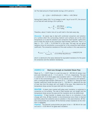
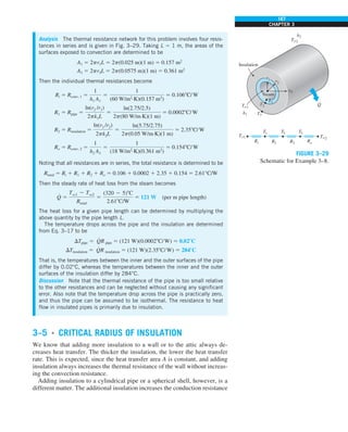
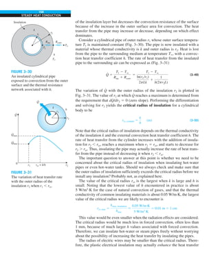
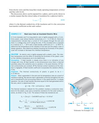
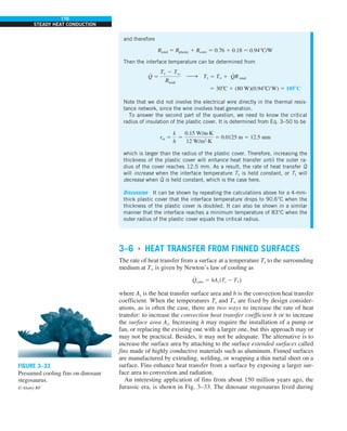
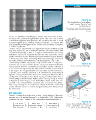

![173
CHAPTER 3
yields zero. Therefore, the general solution of the differential equation
Eq. 3–56 is
u(x) 5 C1emx
1 C2e2mx
(3–58)
where C1 and C2 are arbitrary constants whose values are to be determined
from the boundary conditions at the base and at the tip of the fin. Note that we
need only two conditions to determine C1 and C2 uniquely.
The temperature of the plate to which the fins are attached is normally
known in advance. Therefore, at the fin base we have a specified temperature
boundary condition, expressed as
Boundary condition at fin base: u(0) 5 ub 5 Tb 2 T` (3–59)
At the fin tip we have several possibilities, including infinitely long fins,
negligible heat loss (idealized as an adiabatic tip), specified temperature, and
convection (Fig. 3–37). Next, we consider each case separately.
1 Infinitely Long Fin (Tfin tip 5 T`)
For a sufficiently long fin of uniform cross section (Ac 5 constant), the tem-
perature of the fin at the fin tip approaches the environment temperature T`
and thus u approaches zero. That is,
Boundary condition at fin tip: u(L) 5 T(L) 2 T` 5 0 as L S `
This condition is satisfied by the function e2mx
, but not by the other prospec-
tive solution function emx
since it tends to infinity as x gets larger. Therefore,
the general solution in this case will consist of a constant multiple of e2mx
. The
value of the constant multiple is determined from the requirement that at the
fin base where x 5 0 the value of u is ub. Noting that e2mx
5 e0
5 1, the proper
value of the constant is ub, and the solution function we are looking for is
u(x) 5 ube2mx
. This function satisfies the differential equation as well as the
requirements that the solution reduce to ub at the fin base and approach zero at
the fin tip for large x. Noting that u 5 T 2 T` and m 5 hp/kAc, the variation
of temperature along the fin in this case can be expressed as
Very long fin:
T(x) 2 Tq
Tb 2 Tq
5 e2mx
5 e2xhp/kAc (3–60)
Note that the temperature along the fin in this case decreases exponentially
from Tb to T`, as shown in Fig. 3–38. The steady rate of heat transfer from the
entire fin can be determined from Fourier’s law of heat conduction
Very long fin: Q
#
long fin 5 2kAc
dT
dx
`
x50
5 hpkAc (Tb 2 T`) (3–61)
where p is the perimeter, Ac is the cross-sectional area of the fin, and x is the
distance from the fin base. Alternatively, the rate of heat transfer from the
fin could also be determined by considering heat transfer from a differential
volume element of the fin and integrating it over the entire surface of the fin:
Q
#
fin 5 #Afin
h[T(x) 2 T`] dAfin 5 #Afin
hu(x) dAfin (3–62)
Tb
0
1. Infinitely long fin
2. Negligible heat loss (adiabatic tip)
3. Specified temperature
4. Convection
T`
L
x
FIGURE 3–37
Boundary conditions at the fin base
and the fin tip.
Tb
T`
Tb
T(x) = T` + (Tb – T`)e
T
L
0
x
Ab = Ac
k
h, T`
hp
—–
kAc
–x
D
(p = pD, Ac = pD2
/4 for a cylindrical fin)
FIGURE 3–38
A long circular fin of uniform
cross section and the variation of
temperature along it.](https://image.slidesharecdn.com/25489135-230110133727-3d40a16a/85/25489135-pdf-196-320.jpg)
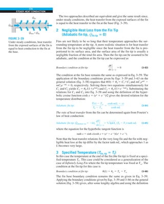
![175
CHAPTER 3
of the hyperbolic sine function, sinh x 5 (ex
2e2x
)/2, the desired temperature
distribution:
Specified fin tip temperature:
T(x) 2 Tq
Tb 2 Tq
5
[(TL 2 Tq)/(Tb 2 Tq)]sinh mx 1 sinh m(L 2 x)
sinh mL
(3–67)
Using the Fourier’s law of heat conduction, the rate of heat transfer from the fin is
Specified fin tip temperature:
Q
.
specified temp. 5 2kAc
dT
dx
`
x50
5 hpkAc(Tb 2 Tq)
cosh mL 2 [(TL 2 Tq)/(Tb 2 Tq)]
sinh mL
(3–68)
Note that Eqs. 3–67 and 3–68 reduce to Eqs. 3–60 and 3–61 for the case of
infinitely long fin (L S `).
4 Convection from Fin Tip
The fin tips, in practice, are exposed to the surroundings, and thus the proper
boundary condition for the fin tip is convection that may also include the
effects of radiation. Consider the case of convection only at the tip. The con-
dition at the fin tip can be obtained from an energy balance at the fin tip
(Q
#
cond 5 Q
#
conv) That is,
Boundary condition at fin tip: 2 kAc
dT
dx
`
x5L
5 hAc[T(L) 2 Tq] (3–69)
The boundary condition at the fin base is Eq. 3–59, which is the same as
the three previous cases. Substituting the two boundary conditions given by
Eqs. 3–59 and 3–69 in the general solution (Eq. 3–58), it may be shown, after
some lengthy manipulation that the temperature distribution is
Convection from fin tip:
T(x) 2 Tq
Tb 2 Tq
5
cosh m(L2x) 1 (h/mk) sinh m(L2x)
cosh mL 1 (h/mk) sinh mL
(3–70)
The rate of heat transfer from the fin can be found by substituting the temper-
ature gradient at the base of the fin, obtained from Eq. 3–70, into the Fourier’s
law of heat conduction. The result is
Convection from fin tip:
Q
#
convection 5 2kAc
dT
dx
`
x50
5 hpkAc (Tb 2 Tq)
sinh mL 1 (h/mk) cosh mL
cosh mL 1 (h/mk) sinh mL
(3–71)
The solution to the general fin equation for the case of convection from
fin tip is rather complex. An approximate, yet practical and accurate, way of
accounting for the loss from the fin tip is to replace the fin length L in the rela-
tion for the insulated tip case by a corrected fin length defined as (Fig. 3–40)
Corrected fin length: Lc 5 L 1
Ac
p
(3–72)
Lc
Insulated
(b) Equivalent fin with insulated tip
Qfin
·
L
Convection
(a) Actual fin with
convection at the tip
Qfin
·
Ac
–—
p
FIGURE 3–40
Corrected fin length Lc is defined such
that heat transfer from a fin of length
Lc with insulated tip is equal to heat
transfer from the actual fin of length L
with convection at the fin tip.](https://image.slidesharecdn.com/25489135-230110133727-3d40a16a/85/25489135-pdf-198-320.jpg)
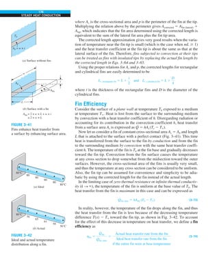
![177
CHAPTER 3
Straight rectangular fins
m 5 2h/kt
Lc 5 L 1 t/2
Afin 5 2wLc
Straight triangular fins
m 5 2h/kt
Afin 5 2wL2
1 (t/2)2
Straight parabolic fins
m 5 2h/kt
Afin 5 wL[C1 1 (L/t)ln(t/L 1 C1)]
C1 5 1 1 (t/L)2
Circular fins of rectangular profile
m 5 2h/kt
r2c 5 r2 1 t/2
Afin 5 2p(r2c
2
2 r1
2
)
Pin fins of rectangular profile
m 5 4h/kD
Lc 5 L 1 D/4
Afin 5 pDLc
Pin fins of triangular profile
m 5 4h/kD
Afin 5
pD
2
L2
1 (D/2)2
Pin fins of parabolic profile
m 5 4h/kD
Afin 5
pL3
8D
[C3C4 2
L
2D
ln(2DC4/L 1 C3)]
C3 5 1 1 2(D/L)2
C4 5 1 1 (D/L)2
Pin fins of parabolic profile
(blunt tip)
m 5 4h/kD
Afin 5
pD4
96L2
e [16(L/D)2
1 1]3/2
2 1f
hfin 5
tanhmLc
mLc
hfin 5
1
mL
I1(2mL)
I1(2mL)
hfin 5
2
1 1 (2mL)2
1 1
hfin 5 C2
K1(mr1)I1(mr2c) 2 I1(mr1)K1(mr2c)
I0(mr1)K1(mr2c) 1 K0(mr1)I1(mr2c)
C2 5
2r1/m
r2c
2
2 r1
2
hfin 5
tanhmLc
mLc
hfin 5
2
mL
I0(2mL)
I1(2mL)
I2 (x) 5 I0 (x) 2 (2/x)I1 (x) where x 5 2mL
hfin 5
2
1 1 (2mL/3)2
1 1
hfin 5
3
2mL
I2(4mL/3)
I0(4mL/3)
TABLE 3–3
Efficiency and surface areas of common fin configurations
w
L
x
t
y = (t/2) (1 – x/L)
t
w
L
t
L
w
y = (t/2) (1 2 x/L)2
r2
r1
t
L
D
L
y = (D/2) (1 – x/L)
D
L
y = (D/2) (1 – x/L)2
D
L
y = (D/2) (1 – x/L)1/2
D
L](https://image.slidesharecdn.com/25489135-230110133727-3d40a16a/85/25489135-pdf-200-320.jpg)
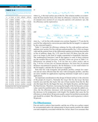
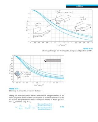
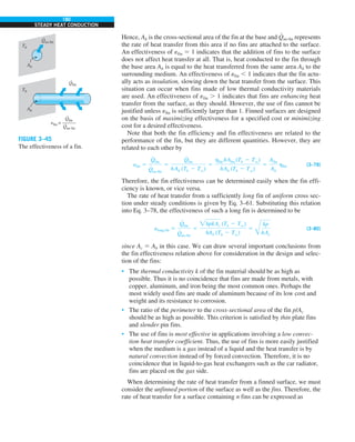
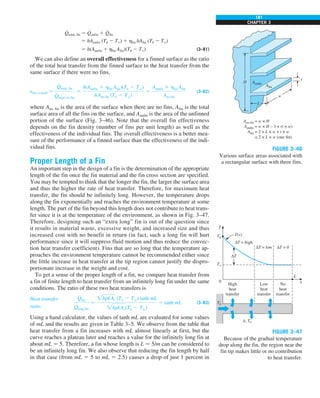
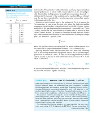
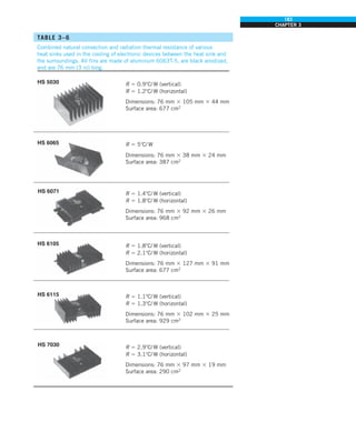
![185
CHAPTER 3
EXAMPLE 3–12 Heat Transfer from Fins of Variable Cross Section
Aluminum pin fins of parabolic profile with blunt tips are attached on a plane
wall with surface temperature of 200°C (Fig. 3–49). Each fin has a length of
20 mm and a base diameter of 5 mm. The fins are exposed to an ambient air
condition of 25°C and the convection heat transfer coefficient is 50 W/m2
·K. If
the thermal conductivity of the fins is 240 W/m2
·K, determine the efficiency,
heat transfer rate, and effectiveness of each fin.
SOLUTION The efficiency, heat transfer rate, and effectiveness of a pin fin of
parabolic profile with blunt tips are to be determined.
Assumptions 1 Heat conduction is steady and one-dimensional. 2 Thermal
properties are constant. 3 Heat transfer by radiation is negligible.
Properties The thermal conductivity of the fin is given as 240 W/m2
·K.
Analysis From Table 3–3, for pin fins of parabolic profile (blunt tip), we have
mL 5
Å
4h
kD
L 5
Å
4(50W/m2
·K)
(240W/m·K)(0.005 m)
(0.020 m) 5 0.2582
Afin 5
pD4
96L2
e c16a
L
D
b
2
1 1d
3/2
2 1f 5
p(0.005 m)4
96(0.020 m)2
e c16a
0.020 m
0.005 m
b
2
1 1d
3/2
2 1f
5 2.106 3 1024
m2
hfin 5
3
2mL
I1(4mL/3)
I0(4mL/3)
5
3
2(0.2582)
I1[4(0.2582)/3]
I0[4(0.2582)/3]
5 5.8095
I1[0.3443]
I0[0.3443]
The values of the Bessel functions corresponding to x 5 0.3443 are deter-
mined from Table 3–4 to be I0 5 1.0350 and I1 5 0.1716. Substituting, the
fin efficiency is determined to be
hfin 5 5.8095
0.1716
1.0350
5 0.9632
The heat transfer rate for a single fin is
Q
#
fin 5 hfin hAfin (Tb 2 Tq)
5 (0.9632)(50W/m2
·K)(2.106 3 1024
m2
)(200 2 25)8C 5 1.77 W
The fin effectiveness is
efin 5
Q
#
fin
hAb(Tb 2 Tq)
5
Q
#
fin
h(pD2
/4)(Tb 2 Tq)
5
1.77 W
(50W/m2
·K) [p(0.005 m)2
/4] (200 2 25)8C
5 10.3
That is, over a 10-fold increase in heat transfer is achieved by using a pin fin
in this case.
L = 20 mm
D = 5 mm
Air, 25°C
h = 50 W/m2
·K
k = 240 W/m·K
Tb = 200°C
FIGURE 3–49
Schematic for Example 3–12.](https://image.slidesharecdn.com/25489135-230110133727-3d40a16a/85/25489135-pdf-208-320.jpg)
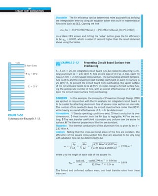
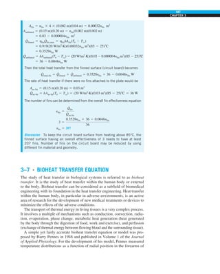
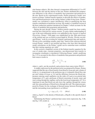
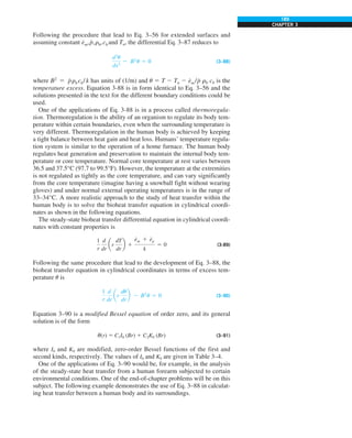
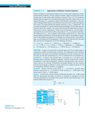
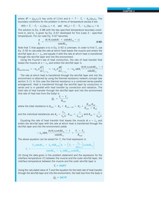
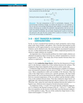
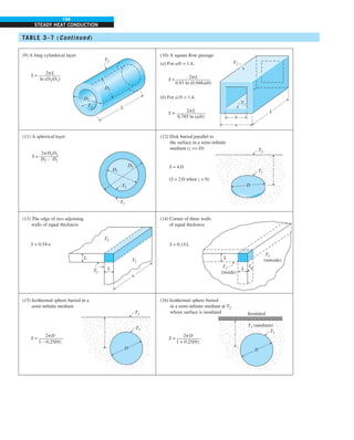
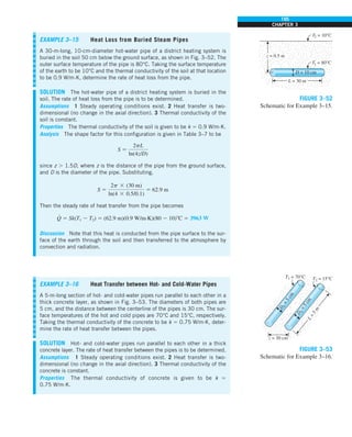
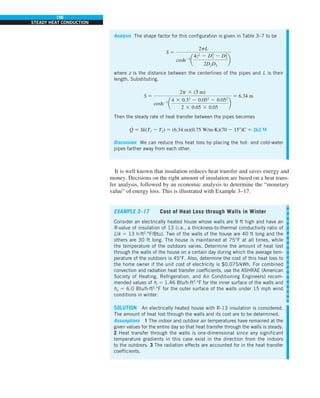
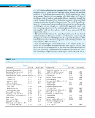
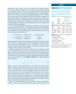
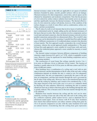
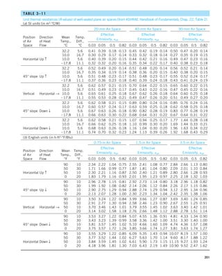
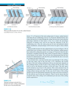
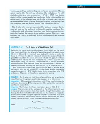
![204
STEADY HEAT CONDUCTION
and the value of the area fraction farea is 0.75 for the insulation section and
0.25 for the stud section since the headers that constitute a small part of the
wall are to be treated as studs. Using the available R-values from Table 3–8
and calculating others, the total R-values for each section can be determined
in a systematic manner in the table below.
Schematic R-value, m2
·°C/W
Between At
Construction Studs Studs
1. Outside surface,
24 km/h wind 0.030 0.030
2. Wood bevel lapped
siding 0.14 0.14
3. Wood fiberboard
sheeting, 13 mm 0.23 0.23
4a. Glass fiber
insulation, 90 mm 2.45 —
4b. Wood stud,
38 mm 3 90 mm — 0.63
5. Gypsum wallboard,
13 mm 0.079 0.079
6. Inside surface, still air 0.12 0.12
Total unit thermal resistance of each section, R
(in m2
·°C/W) 3.05 1.23
The U-factor of each section, U 5 1/R, in W/m2
·K 0.328 0.813
Area fraction of each section, farea 0.75 0.25
Overall U-factor: U 5 ofarea, i Ui 5 0.75 3 0.328 1 0.25 3 0.813
5 0.449 W/m2
·K
Overall unit thermal resistance: R 5 1/U 5 2.23 m2
·°C/W
We conclude that the overall unit thermal resistance of the wall is
2.23 m2
·°C/W, and this value accounts for the effects of the studs and head-
ers. It corresponds to an R-value of 2.23 3 5.68 5 12.7 (or nearly R-13) in
English units. Note that if there were no wood studs and headers in the wall,
the overall thermal resistance would be 3.05 m2
·°C/W, which is 37 percent
greater than 2.23 m2
·°C/W. Therefore, the wood studs and headers in this case
serve as thermal bridges in wood frame walls, and their effect must be consid-
ered in the thermal analysis of buildings.
The perimeter of the building is 50 m and the height of the walls is 2.5 m.
Noting that glazing constitutes 20 percent of the walls, the total wall area is
Awall 5 0.80(Perimeter)(Height) 5 0.80(50 m)(2.5 m) 5 100 m2
Then the rate of heat loss through the walls under design conditions becomes
Q
·
wall 5 (UA)wall (Ti 2 To)
5 (0.449 W/m2
·K)(100 m2
)[22 2 (22)°C]
5 1078 W
Discussion Note that a 1-kW resistance heater in this house will make up
almost all the heat lost through the walls, except through the doors and
windows, when the outdoor air temperature drops to 22°C.
4a
1
3
2
4b
5
6](https://image.slidesharecdn.com/25489135-230110133727-3d40a16a/85/25489135-pdf-227-320.jpg)
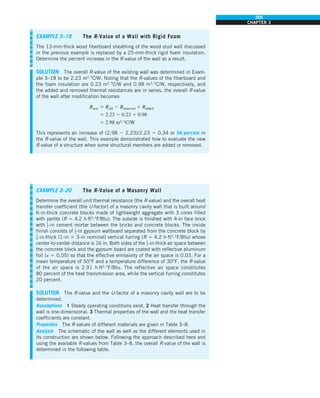
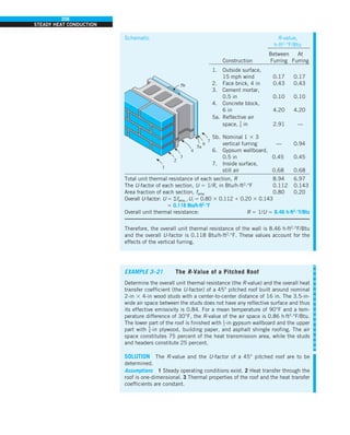
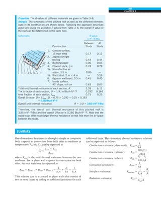
![208
STEADY HEAT CONDUCTION
where hc is the thermal contact conductance, Rc is the thermal
contact resistance, and the radiation heat transfer coefficient
is defined as
hrad 5 es(T2
s 1 T2
surr)(Ts 1 Tsurr)
Once the rate of heat transfer is available, the temperature
drop across any layer can be determined from
DT 5 Q
#
R
The thermal resistance concept can also be used to solve steady
heat transfer problems involving parallel layers or combined
series-parallel arrangements.
Adding insulation to a cylindrical pipe or a spherical shell
increases the rate of heat transfer if the outer radius of the insu-
lation is less than the critical radius of insulation, defined as
rcr, cylinder 5
kins
h
rcr, sphere 5
2kins
h
The effectiveness of an insulation is often given in terms
of its R-value, the thermal resistance of the material for a unit
surface area, expressed as
R-value 5
L
k
(flat insulation)
where L is the thickness and k is the thermal conductivity of
the material.
Finned surfaces are commonly used in practice to enhance
heat transfer. Fins enhance heat transfer from a surface by
exposing a larger surface area to convection. The temperature
distribution along the fin are given by
Very long fin:
T(x) 2 Tq
Tb 2 Tq
5 e2xhp/kAc
Adiabatic fin tip:
T(x) 2 Tq
Tb 2 Tq
5
cosh m(L 2 x)
cosh mL
Specified temperature at fin tip:
T(x) 2 Tq
Tb 2 Tq
5
[(TL 2 Tq)/(Tb 2 Tq)]sinh mx 1 sinh m(L 2 x)
sinhmL
Convection from fin tip:
T(x) 2 Tq
Tb 2 Tq
5
coshm(L 2 x) 1 (h/mk) sinhm(L 2 x)
coshmL 1 (h/mk) sinh mL
where m 5 hp/kAc, p is the perimeter, and Ac is the cross-
sectional area of the fin. The rates of heat transfer for these
cases are given to be
Very long fin:
Q
#
long fin 5 2kAc
dT
dx
`
x50
5 hpk Ac (Tb 2 Tq)
Adiabatic fin tip:
Q
#
adiabatic tip 5 2kAc
dT
dx
`
x50
5 hpkAc (Tb 2 Tq) tanh mL
Specified temperature at fin tip:
Q
#
specified temp. 5 hpkAc(Tb 2 Tq)
coshmL 2 [(TL 2 Tq)/(Tb 2 Tq)]
sinhmL
Convection from the fin tip:
Q
#
convection 5 hpkAc (Tb 2 Tq)
sinhmL 1 (h/mk)coshmL
coshmL 1 (h/mk)sinhmL
Fins exposed to convection at their tips can be treated as fins
with adiabatic tips by using the corrected length Lc 5 L 1 Ac/p
instead of the actual fin length.
The temperature of a fin drops along the fin, and thus the heat
transfer from the fin is less because of the decreasing tempera-
ture difference toward the fin tip. To account for the effect of this
decrease in temperature on heat transfer, we define fin efficiency as
hfin 5
Q
#
fin
Q
#
fin, max
5
Actual heat transfer rate from the fin
Ideal heat transfer rate from the fin if
the entire fin were at base temperature
When the fin efficiency is available, the rate of heat transfer
from a fin can be determined from
Q
#
fin 5 hfinQ
#
fin, max 5 hfinhAfin (Tb 2 T`)
The performance of the fins is judged on the basis of the
enhancement in heat transfer relative to the no-fin case and is
expressed in terms of the fin effectiveness efin, defined as
efin 5
Q
#
fin
Q
#
no fin
5
Q
#
fin
hAb (Tb 2 Tq)
5
Heat transfer rate from
the fin of base area Ab
Heat transfer rate from
the surface of area Ab
Here, Ab is the cross-sectional area of the fin at the base and
Q
#
no fin represents the rate of heat transfer from this area if no
fins are attached to the surface. The overall effectiveness for
a finned surface is defined as the ratio of the total heat transfer
from the finned surface to the heat transfer from the same sur-
face if there were no fins,
efin, overall 5
Q
#
total, fin
Q
#
total, no fin
5
h(Aunfin 1 hfin Afin)(Tb 2 Tq)
hAno fin (Tb 2 Tq)
Fin efficiency and fin effectiveness are related to each other by
efin 5
Afin
Ab
hfin
Certain multidimensional heat transfer problems involve two
surfaces maintained at constant temperatures T1 and T2. The steady
rate of heat transfer between these two surfaces is expressed as
Q
#
5 Sk(T1 2 T2)
where S is the conduction shape factor that has the dimension
of length and k is the thermal conductivity of the medium
between the surfaces.](https://image.slidesharecdn.com/25489135-230110133727-3d40a16a/85/25489135-pdf-231-320.jpg)
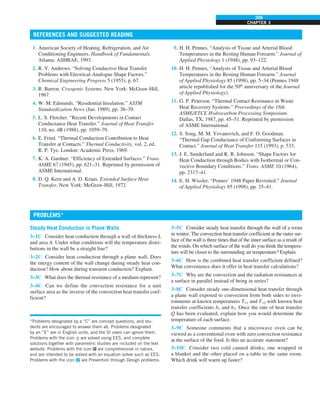
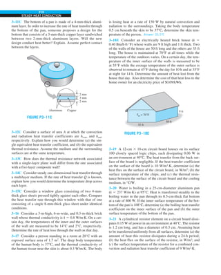
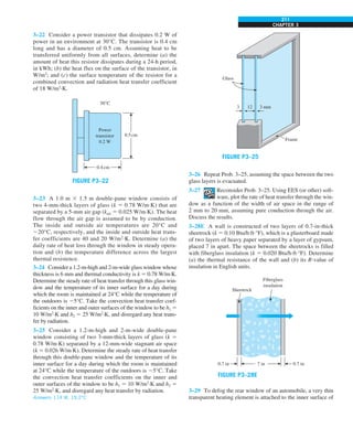
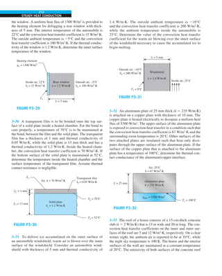
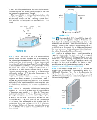
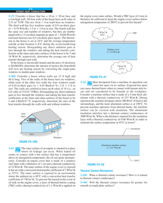
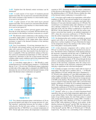
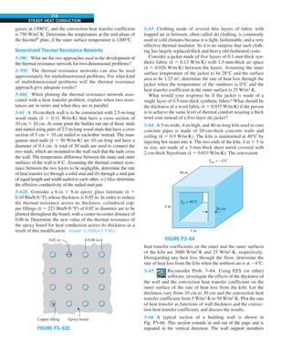
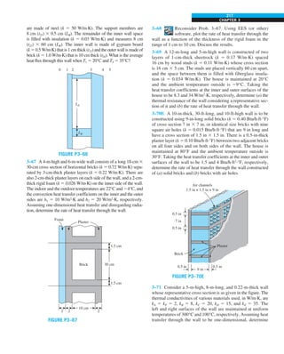
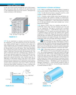
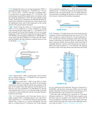
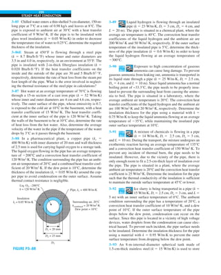
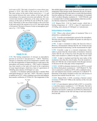
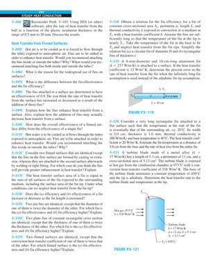
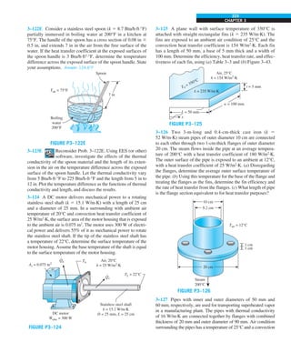
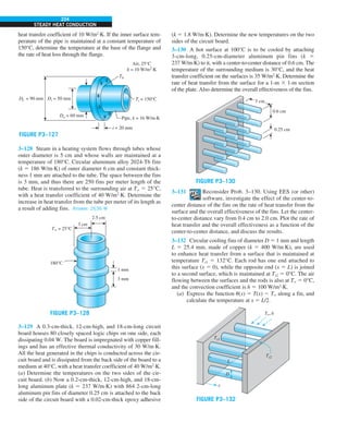
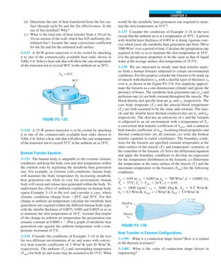
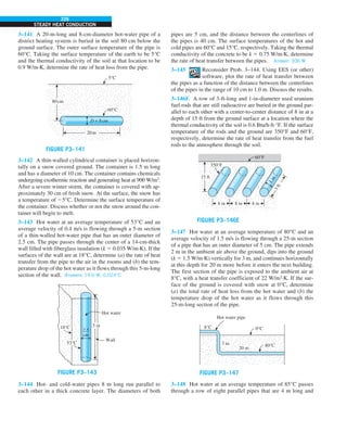
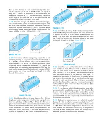
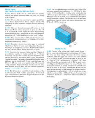
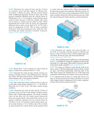
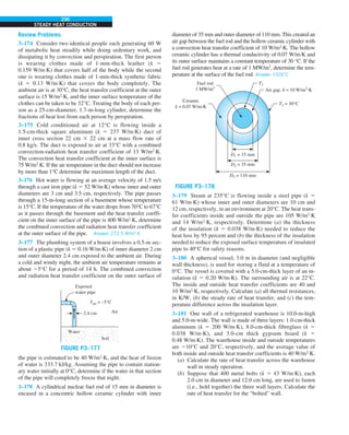
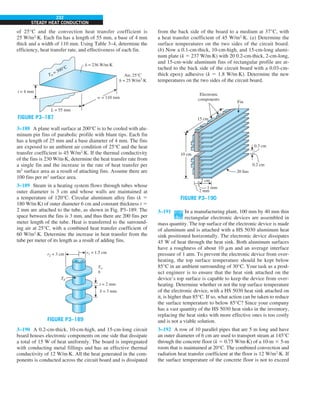
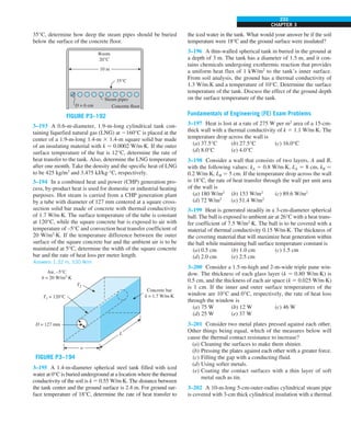
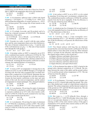
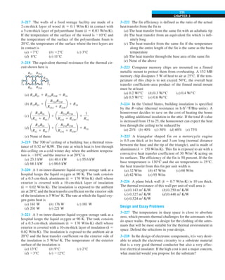
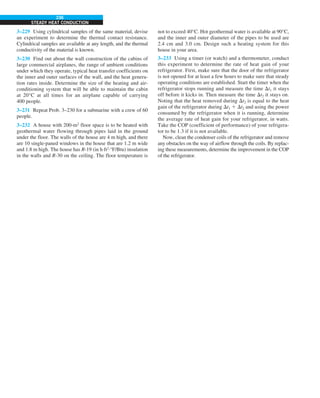
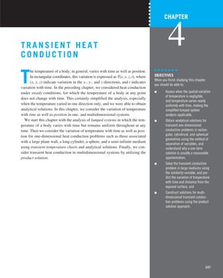
![238
TRANSIENT HEAT CONDUCTION
4–1 ■
LUMPED SYSTEM ANALYSIS
In heat transfer analysis, some bodies are observed to behave like a “lump”
whose interior temperature remains essentially uniform at any times during
a heat transfer process. The temperature of such bodies can be taken to be a
function of time only, T(t). Heat transfer analysis that utilizes this idealiza-
tion is known as lumped system analysis, which provides great simplifica-
tion in certain classes of heat transfer problems without much sacrifice from
accuracy.
Consider a small hot copper ball coming out of an oven (Fig. 4–1). Mea-
surements indicate that the temperature of the copper ball changes with time,
but it does not change much with position at any given time. Thus the tem-
perature of the ball remains nearly uniform at all times, and we can talk about
the temperature of the ball with no reference to a specific location.
Now let us go to the other extreme and consider a large roast in an oven. If
you have done any roasting, you must have noticed that the temperature dis-
tribution within the roast is not even close to being uniform. You can easily
verify this by taking the roast out before it is completely done and cutting it
in half. You will see that the outer parts of the roast are well done while the
center part is barely warm. Thus, lumped system analysis is not applicable in
this case. Before presenting a criterion about applicability of lumped system
analysis, we develop the formulation associated with it.
Consider a body of arbitrary shape of mass m, volume V, surface area As,
density r, and specific heat cp initially at a uniform temperature Ti (Fig. 4–2).
At time t 5 0, the body is placed into a medium at temperature T`, and heat
transfer takes place between the body and its environment, with a heat trans-
fer coefficient h. For the sake of discussion, we assume that T` . Ti, but the
analysis is equally valid for the opposite case. We assume lumped system
analysis to be applicable, so that the temperature remains uniform within the
body at all times and changes with time only, T 5 T(t).
During a differential time interval dt, the temperature of the body rises by
a differential amount dT. An energy balance of the solid for the time interval
dt can be expressed as
Heat transfer into the body
during dt 5
The increase in the
energy of the body
during dt
or
hAs(T` 2 T) dt 5 mcp dT (4–1)
Noting that m 5 rV and dT 5 d(T 2 T`) since T` 5 constant, Eq. 4–1 can be
rearranged as
d(T 2 Tq)
T 2 Tq
5 2
hAs
rVcp
dt (4–2)
Integrating from t 5 0, at which T 5 Ti,to any time t, at which T 5 T(t), gives
ln
T(t) 2 Tq
Ti 2 Tq
5 2
hAs
rVcp
t (4–3)
¢ ≤
£ ≥
Solid body
m = mass
V = volume
r = density
Ti = initial temperature
T = T(t)
= hAs[T` – T(t)]
As
h
T`
Q
·
FIGURE 4–2
The geometry and parameters involved
in the lumped system analysis.
FIGURE 4–1
A small copper ball can be modeled
as a lumped system, but a roast
beef cannot.
70°C
70°C
70°C
70°C
70°C
(a) Copper ball
(b) Roast beef
110°C
90°C
40°C](https://image.slidesharecdn.com/25489135-230110133727-3d40a16a/85/25489135-pdf-261-320.jpg)
![239
CHAPTER 4
Taking the exponential of both sides and rearranging, we obtain
T(t) 2 Tq
Ti 2 Tq
5 e2bt
(4–4)
where
b 5
hAs
rVcp
(1/s) (4–5)
is a positive quantity whose dimension is (time)21
. The reciprocal of b has
time unit (usually s), and is called the time constant. Equation 4–4 is plotted
in Fig. 4–3 for different values of b. There are two observations that can be
made from this figure and the relation above:
1. Equation 4–4 enables us to determine the temperature T(t) of a body at
time t, or alternatively, the time t required for the temperature to reach
a specified value T(t).
2. The temperature of a body approaches the ambient temperature T` expo-
nentially. The temperature of the body changes rapidly at the beginning,
but rather slowly later on. A large value of b indicates that the body
approaches the environment temperature in a short time. The larger the
value of the exponent b, the higher the rate of decay in temperature.
Note that b is proportional to the surface area, but inversely proportional
to the mass and the specific heat of the body. This is not surprising since
it takes longer to heat or cool a larger mass, especially when it has a
large specific heat.
Once the temperature T(t) at time t is available from Eq. 4–4, the rate of con-
vection heat transfer between the body and its environment at that time can be
determined from Newton’s law of cooling as
Q
·
(t) 5 hAs[T(t) 2 T`] (W) (4–6)
The total amount of heat transfer between the body and the surrounding
medium over the time interval t 5 0 to t is simply the change in the energy
content of the body:
Q 5 mcp[T(t) 2 Ti] (kJ) (4–7)
The amount of heat transfer reaches its upper limit when the body reaches the
surrounding temperature T`. Therefore, the maximum heat transfer between
the body and its surroundings is (Fig. 4–4)
Qmax 5 mcp(T` 2 Ti) (kJ) (4–8)
We could also obtain this equation by substituting the T(t) relation from
Eq. 4–4 into the Q
·
(t) relation in Eq. 4–6 and integrating it from t 5 0 to t S `.
Criteria for Lumped System Analysis
The lumped system analysis certainly provides great convenience in heat
transfer analysis, and naturally we would like to know when it is appropriate
FIGURE 4–3
The temperature of a lumped
system approaches the environment
temperature as time gets larger.
T(t)
T`
Ti
b3
b3 b2 b1
b2
b1
t
FIGURE 4–4
Heat transfer to or from a body
reaches its maximum value
when the body reaches
the environment temperature.
Ti
Ti
Q = Qmax = mcp (Ti – T`)
h
T`
t = 0 t → `
Ti
Ti
Ti
Ti
Ti
T`
T`
T`
T`
T`
T`
T`](https://image.slidesharecdn.com/25489135-230110133727-3d40a16a/85/25489135-pdf-262-320.jpg)
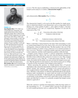
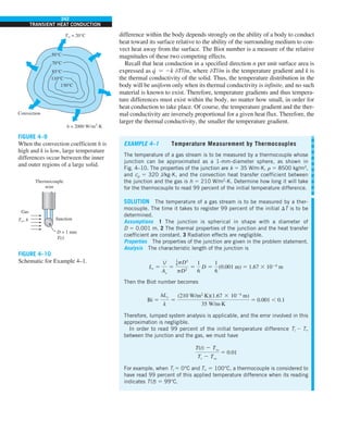
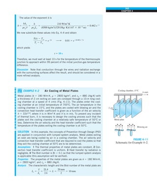
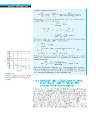
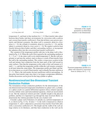
![246
TRANSIENT HEAT CONDUCTION
approximated to be one-dimensional. Also, there is thermal symmetry about
the midplane passing through x 5 0, and thus the temperature distribution
must be symmetrical about the midplane. Therefore, the value of temperature
at any 2x value in 2L # x # 0 at any time t must be equal to the value at 1x in
0 # x # L at the same time. This means we can formulate and solve the heat
conduction problem in the positive half domain 0 # x # L, and then apply the
solution to the other half.
Under the conditions of constant thermophysical properties, no heat genera-
tion, thermal symmetry about the midplane, uniform initial temperature, and
constant convection coefficient, the one-dimensional transient heat conduc-
tion problem in the half-domain 0 # x # L of the plane wall can be expressed
as (see Chapter 2)
Differential equation:
02
T
0x2
5
1
a
0T
0t
(4–10a)
Boundary conditions:
0T(0, t)
0x
5 0 and 2k
0T(L, t)
0x
5 h[T(L, t) 2 Tq] (4–10b)
Initial condition: T(x, 0) 5 Ti (4–10c)
where the property a 5 k/rcp is the thermal diffusivity of the material.
We now attempt to nondimensionalize the problem by defining a
dimensionless space variable X 5 x/L and dimensionless temperature u(x, t) 5
[T(x, t) 2 T`]/[Ti 2 T`]. These are convenient choices since both X and u vary
between 0 and 1. However, there is no clear guidance for the proper form of
the dimensionless time variable and the h/k ratio, so we will let the analysis
indicate them. We note that
0u
0X
5
0u
0(x/L)
5
L
Ti 2 Tq
0T
0x
, 02
u
0X2
5
L2
Ti 2 Tq
02
T
0x2
and
0u
0t
5
1
Ti 2 Tq
0T
0t
Substituting into Eqs. 4–10a and 4–10b and rearranging give
02
u
0X2
5
L2
a
0u
0t
and
0u(1, t)
0X
5
hL
k
u(1, t) (4–11)
Therefore, the proper form of the dimensionless time is t 5 at/L2
, which is
called the Fourier number Fo (named after Jean Baptiste Joseph Fourier,
see Fig. 1–27), and we recognize Bi 5 k/hL as the Biot number defined in
Section 4–1. Then the formulation of the one-dimensional transient heat con-
duction problem in a plane wall can be expressed in nondimensional form as
Dimensionless differential equation:
02
u
0X2
5
0u
0t
(4–12a)
Dimensionless BC’s:
0u(0, t)
0X
5 0 and
0u(1, t)
0X
5 2Biu(1, t)
(4–12b)
Dimensionless initial condition: u(X, 0) 5 1 (4–12c)
where
u(X, t) 5
T(x, t) 2 Tq
Ti 2 Tq
Dimensionless temperature
X 5
x
L
Dimensionless distance from the center](https://image.slidesharecdn.com/25489135-230110133727-3d40a16a/85/25489135-pdf-269-320.jpg)
![247
CHAPTER 4
Bi 5
hL
k
Dimensionless heat transfer coefficient (Biot number)
t 5
at
L2
5 Fo Dimensionless time (Fourier number)
The heat conduction equation in cylindrical or spherical coordinates can
be nondimensionalized in a similar way. Note that nondimensionalization
reduces the number of independent variables and parameters from 8 to 3—
from x, L, t, k, a, h, Ti, and T` to X, Bi, and Fo (Fig. 4–15). That is,
u 5 f(X, Bi, Fo) (4–13)
This makes it very practical to conduct parametric studies and avoid results
in graphical form. Equation 4–13 is the generalized version of Eq. 4–4 for the
lumped system analysis (no space variables). This can be shown by using the
definitions of u, a, Lc, Bi, and Fo in Eq. 4–4. The final result is
u 5
T(t) 2 Tq
Ti 2 Tq
5 e2bt
5 e
2
hAst
rVcp
5 e2BiFo
or u 5 f(Fo, Bi) which is the special case of Eq. 4–13 with no space variable.
Exact Solution of One-Dimensional
Transient Conduction Problem*
The non-dimensionalized partial differential equation given in Eqs. 4–12
together with its boundary and initial conditions can be solved using several
analytical and numerical techniques, including the Laplace or other transform
methods, the method of separation of variables, the finite difference method, and
the finite-element method. Here we use the method of separation of variables
developed by J. Fourier in the 1820s and is based on expanding an arbitrary
function (including a constant) in terms of Fourier series. The method is applied
by assuming the dependent variable to be a product of a number of functions,
each being a function of a single independent variable. This reduces the partial
differential equation to a system of ordinary differential equations, each being a
function of a single independent variable. In the case of transient conduction in
a plane wall, for example, the dependent variable is the solution function u(X, t),
which is expressed as u(X, t) 5 F(X)G(t), and the application of the method
results in two ordinary differential equation, one in X and the other in t.
The method is applicable if (1) the geometry is simple and finite (such as a rectan-
gular block, a cylinder, or a sphere) so that the boundary surfaces can be described
by simple mathematical functions, and (2) the differential equation and the bound-
ary and initial conditions in their most simplified form are linear (no terms that
involve products of the dependent variable or its derivatives) and involve only one
nonhomogeneous term (a term without the dependent variable or its derivatives). If
the formulation involves a number of nonhomogeneous terms, the problem can be
split up into an equal number of simpler problems each involving only one nonho-
mogeneous term, and then combining the solutions by superposition.
Now we demonstrate the use of the method of separation of variables by
applying it to the one-dimensional transient heat conduction problem given in
*This section can be skipped if desired without a loss of continuity.
FIGURE 4–15
Nondimensionalization reduces
the number of independent variables in
one-dimensional transient conduction
problems from 8 to 3, offering great
convenience in the presentation
of results.
02
T
0x2
0T
0x
1
a
= , T(x, 0) = Ti
, u(X, 0) = 1
T = F(x, L, t, k, a, h, Ti, T`)
0T(0, t)
0x
0T(L, t)
0x
= 0, –k = h[T(L, t) –T`]
02
u
0X2
0u
0t
=
u = f(X, Bi, t)
= –Biu(l, t)
0u(l, t)
0X
= 0,
0u(0, t)
0X
(a) Original heat conduction problem:
(b) Nondimensionalized problem:](https://image.slidesharecdn.com/25489135-230110133727-3d40a16a/85/25489135-pdf-270-320.jpg)
![248
TRANSIENT HEAT CONDUCTION
Eqs. 4–12. First, we express the dimensionless temperature function u(X, t)
as a product of a function of X only and a function of t only as
u(X, t) 5 F(X)G(t) (4–14)
Substituting Eq. 4–14 into Eq. 4–12a and dividing by the product FG gives
1
F
d2
F
dX2
5
1
G
dG
dt
(4–15)
Observe that all the terms that depend on X are on the left-hand side of the equation
and all the terms that depend on t are on the right-hand side. That is, the terms that
are function of different variables are separated (and thus the name separation of
variables). The left-hand side of this equation is a function of X only and the right-
hand side is a function of only t. Considering that both X and t can be varied inde-
pendently,theequalityinEq.4–15canholdforanyvalueofXandtonlyifEq.4–15
is equal to a constant. Further, it must be a negative constant that we will indicate by
2l2
sinceapositiveconstantwillcausethefunctionG(t)toincreaseindefinitelywith
time (to be infinite), which is unphysical, and a value of zero for the constant means
no time dependence, which is again inconsistent with the physical problem. Setting
Eq. 4–15 equal to 2l2
gives
d2
F
dX2
1 l2
F 5 0 and
dG
dt
1 l2
G 5 0 (4–16)
whose general solutions are
F 5 C1 cos(lX) 1 C2 sin(lX) and G 5 C3e2l2
t
(4–17)
and
u 5 FG 5 C3e2l2
t
[C1 cos(lX) 1 C2 sin(lX)] 5 e2l2
t
[A cos(lX) 1 B sin(lX)]
(4–18)
where A 5 C1C3 and B 5 C2C3 are arbitrary constants. Note that we need to
determine only A and B to obtain the solution of the problem.
Applying the boundary conditions in Eq. 4–12b gives
0u(0, t)
0X
5 0 S 2e2l2
t
(Alsin0 1 Blcos0) 5 S B 5 0 S u 5 Ae2l2
t
cos(lX)
0u(1, t)
0X
5 2Biu(1, t) S 2Ae2l2
t
lsinl 5 2BiAe2l2
t
cos l S l tan l 5 Bi
But tangent is a periodic function with a period of p, and the equation
ltanl 5 Bi has the root l1 between 0 and p, the root l2 between p and 2p,
the root ln between (n21)p and np, etc. To recognize that the transcendental
equation l tan l 5 Bi has an infinite number of roots, it is expressed as
lntanln 5 Bi (4–19)
Eq. 4–19 is called the characteristic equation or eigenfunction, and its
roots are called the characteristic values or eigenvalues. The characteristic
equation is implicit in this case, and thus the characteristic values need to be
determined numerically. Then it follows that there are an infinite number of
solutions of the form Ae2l2
t
cos(lX), and the solution of this linear heat con-
duction problem is a linear combination of them,
u 5 a
q
n51
Ane2l2
nt
cos(ln X) (4–20)](https://image.slidesharecdn.com/25489135-230110133727-3d40a16a/85/25489135-pdf-271-320.jpg)
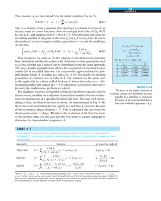
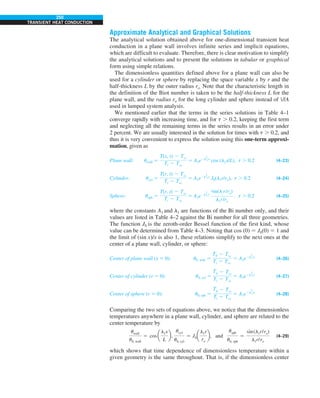
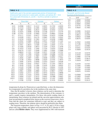
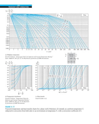
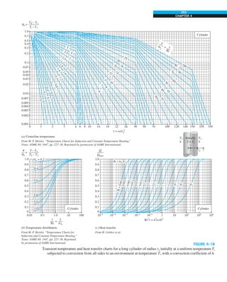
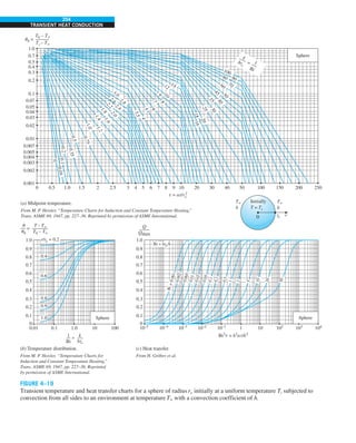
![255
CHAPTER 4
heat transfer charts by H. Gröber. There are three charts associated with each
geometry: the first chart is to determine the temperature T0 at the center of the
geometry at a given time t. The second chart is to determine the temperature
at other locations at the same time in terms of T0. The third chart is to deter-
mine the total amount of heat transfer up to the time t. These plots are valid
for t . 0.2.
Note that the case 1/Bi 5 k/hL 5 0 corresponds to h S `, which corresponds
to the case of specified surface temperature T`. That is, the case in which the
surfaces of the body are suddenly brought to the temperature T` at t 5 0 and
kept at T` at all times can be handled by setting h to infinity (Fig. 4–20).
The temperature of the body changes from the initial temperature Ti to the
temperature of the surroundings T` at the end of the transient heat conduction
process. Thus, the maximum amount of heat that a body can gain (or lose if
Ti . T`) is simply the change in the energy content of the body. That is,
Qmax 5 mcp(T` 2 Ti) 5 rVcp(T` 2 Ti) (kJ) (4–30)
where m is the mass, V is the volume, r is the density, and cp is the specific heat
of the body. Thus, Qmax represents the amount of heat transfer for t S `.
The amount of heat transfer Q at a finite time t is obviously less than this
maximum, and it can be expressed as the sum of the internal energy changes
throughout the entire geometry as
Q 5 #V
rcp[T(x,t) 2 Ti]dV (4–31)
where T(x, t) is the temperature distribution in the medium at time t. Assum-
ing constant properties, the ratio of Q/Qmax becomes
Q
Qmax
5
eV
rcp[T(x, t) 2 Ti]dV
rcp(Tq 2 Ti)V
5
1
V#V
(1 2 u)dV (4–32)
Using the appropriate nondimensional temperature relations based on the one-
term approximation for the plane wall, cylinder, and sphere, and performing
the indicated integrations, we obtain the following relations for the fraction of
heat transfer in those geometries:
Plane wall: a
Q
Qmax
b
wall
5 1 2 u0, wall
sin l1
l1
(4–33)
Cylinder: a
Q
Qmax
b
cyl
5 1 2 2u0, cyl
J1(l1)
l1
(4–34)
Sphere: a
Q
Qmax
b
sph
5 1 2 3u0, sph
sin l1 2 l1 cos l1
l3
1
(4–35)
These Q/Qmax ratio relations based on the one-term approximation are also
plotted in Figures 4–17c, 4–18c, and 4–19c, against the variables Bi and h2
at/k2
for
the large plane wall, long cylinder, and sphere, respectively. Note that once
the fraction of heat transfer Q/Qmax has been determined from these charts or
equations for the given t, the actual amount of heat transfer by that time can
be evaluated by multiplying this fraction by Qmax. A negative sign for Qmax
indicates that the body is rejecting heat (Fig. 4–21).
FIGURE 4–20
The specified surface
temperature corresponds to the case
of convection to an environment at
T` with a convection coefficient h
that is infinite.
Ts
Ts ≠ T`
Ts = T`
Ts
Ts Ts
T`
T`
h
h
h → `
(a) Finite convection coefficient
(b) Infinite convection coefficient
h → `](https://image.slidesharecdn.com/25489135-230110133727-3d40a16a/85/25489135-pdf-278-320.jpg)
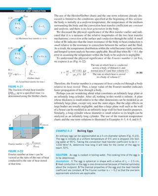
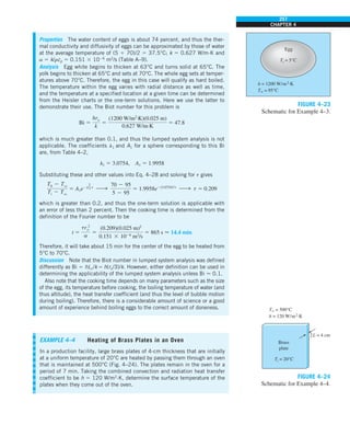
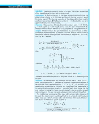
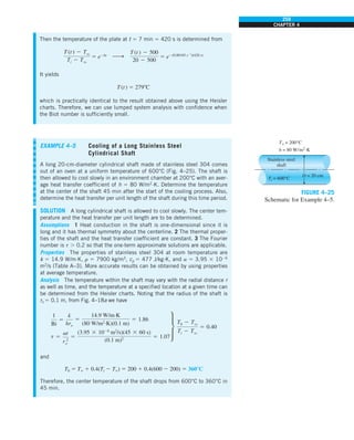
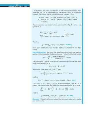
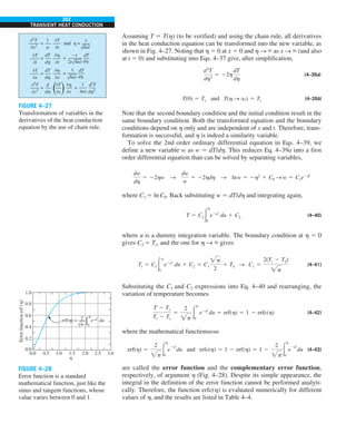
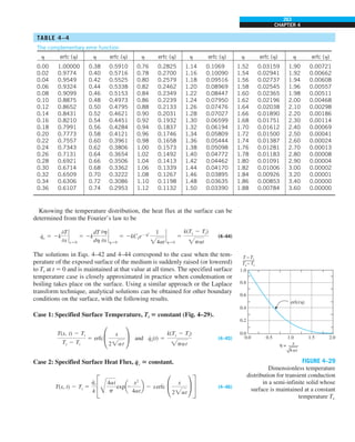
![264
TRANSIENT HEAT CONDUCTION
Case 3: Convection on the Surface, q
#
s(t) 5 h[T` 2 T(0, t)].
T(x,t) 2 Ti
Tq 2 Ti
5 erfc °
x
2at
¢ 2 exp a
hx
k
1
h2
at
k2
berfc °
x
2at
1
hat
k
¢
(4–47)
Case 4: Energy Pulse at Surface, es 5 constant.
Energy in the amount of es per unit surface area (in J/m2
) is supplied to
the semi-infinite body instantaneously at time t 5 0 (by a laser pulse, for
example), and the entire energy is assumed to enter the body, with no heat
loss from the surface.
T(x, t) 2 Ti 5
es
kpt/a
exp a2
x2
4at
b (4–48)
Note that Cases 1 and 3 are closely related. In Case 1, the surface x 5 0 is
brought to a temperature Ts at time t 5 0, and kept at that value at all times. In
Case 3, the surface is exposed to convection by a fluid at a constant tempera-
ture T` with a heat transfer coefficient h.
The solutions for all four cases are plotted in Fig. 4–30 for a representative
case using a large cast iron block initially at 0°C throughout. In Case 1, the
surface temperature remains constant at the specified value of Ts, and tem-
perature increases gradually within the medium as heat penetrates deeper into
the solid. Note that during initial periods only a thin slice near the surface is
affected by heat transfer. Also, the temperature gradient at the surface and
thus the rate of heat transfer into the solid decreases with time. In Case 2,
heat is continually supplied to the solid, and thus the temperature within the
solid, including the surface, increases with time. This is also the case with
convection (Case 3), except that the surrounding fluid temperature T` is the
highest temperature that the solid body can rise to. In Case 4, the surface is
subjected to an instant burst of heat supply at time t 5 0, such as heating by
a laser pulse, and then the surface is covered with insulation. The result is an
instant rise in surface temperature, followed by a temperature drop as heat is
conducted deeper into the solid. Note that the temperature profile is always
normal to the surface at all times. (Why?)
The variation of temperature with position and time in a semi-infinite solid
subjected to convection heat transfer is plotted in Fig. 4–31 for the nondi-
mensionalized temperature against the dimensionless similarity variable
h 5 x/!4at for various values of the parameter h!at / k. Although the
graphical solution given in Fig. 4–31 is simply a plot of the exact analyti-
cal solution, it is subject to reading errors, and thus is of limited accuracy
compared to the analytical solution. Also, the values on the vertical axis of
Fig. 4–31 correspond to x 5 0, and thus represent the surface temperature.
The curve h!at / k 5 ` corresponds to h S `, which corresponds to the case
of specified temperature T` at the surface at x 5 0. That is, the case in which
the surface of the semi-infinite body is suddenly brought to temperature T` at
t 5 0 and kept at T` at all times can be handled by setting h to infinity. For a
finite heat transfer coefficient h, the surface temperature approaches the fluid
temperature T` as the time t approaches infinity.](https://image.slidesharecdn.com/25489135-230110133727-3d40a16a/85/25489135-pdf-287-320.jpg)
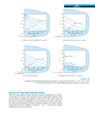
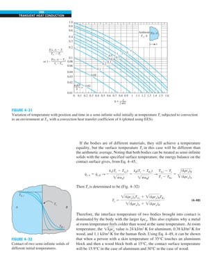
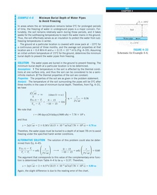
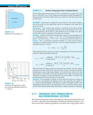
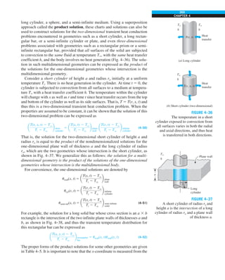
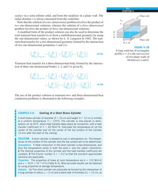
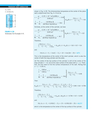
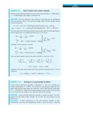
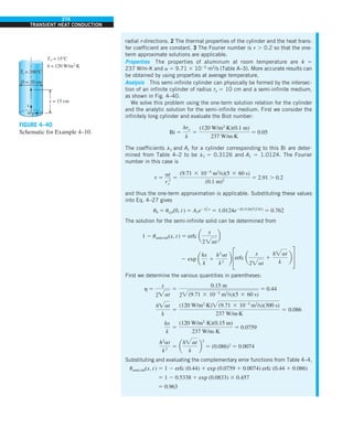
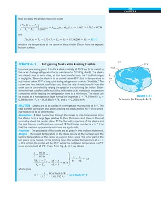
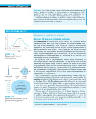
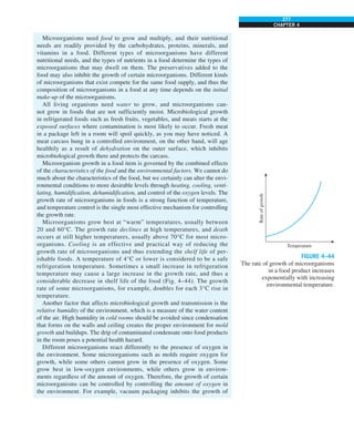
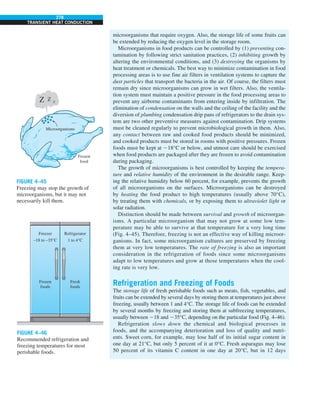
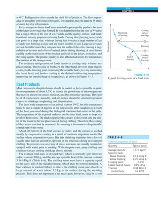
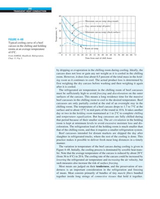
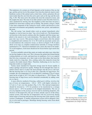
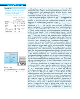
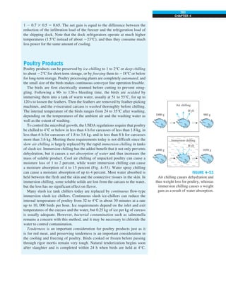
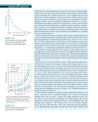
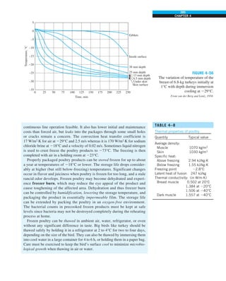
![287
CHAPTER 4
In this chapter, we considered the variation of temperature
with time as well as position in one- or multidimensional
systems. We first considered the lumped systems in which the
temperature varies with time but remains uniform throughout
the system at any time. The temperature of a lumped body
of arbitrary shape of mass m, volume V, surface area As,
density r, and specific heat cp initially at a uniform tem-
perature Ti that is exposed to convection at time t 5 0 in a
medium at temperature T` with a heat transfer coefficient h
is expressed as
T(t) 2 Tq
Ti 2 Tq
5 e2bt
where
b 5
hAs
rcp V
5
h
rcp Lc
(b) Heat is transferred to air at the rate determined above, and the tempera-
ture of the air rises from 22°C to 0.7°C as a result. Therefore, the mass flow
rate of air is
m
·
air 5
#
Qair
(cpDTair)
5
277 kW
(1.006 kJ/kg·K)[0.7 2 (22)8C]
5 102.0 kg/s
Then the volume flow rate of air becomes
V
·
air 5
m
#
air
rair
5
102 kg/s
1.292 kg/m3
5 78.9 m3
/s
(c) Normally the heat transfer load of the evaporator is the same as the refrig-
eration load. But in this case the water that enters the evaporator as a liquid is
frozen as the temperature drops to 22°C, and the evaporator must also remove
the latent heat of freezing, which is determined from
Q
·
freezing 5 (m
· hlatent)water 5 (0.080 kg/s)(333.7 kJ/kg) 5 27 kW
Therefore, the total rate of heat removal at the evaporator is
Q
·
evaporator 5 Q
·
total, chill room 1 Q
·
freezing 5 277 1 27 5 304 kW
Then the heat transfer surface area of the evaporator on the air side is
determined from Q
·
evaporator 5 (UA)air sideDT,
A 5
Q
#
evaporator
UDT
5
304,000 W
(20 W/m2
·K)(5.58C)
5 2764 m2
Obviously, a finned surface must be used to provide such a large surface area
on the air side.
SUMMARY
is a positive quantity whose dimension is (time)21
. This rela-
tion can be used to determine the temperature T(t) of a body
at time t or, alternatively, the time t required for the temper-
ature to reach a specified value T(t). Once the temperature
T(t) at time t is available, the rate of convection heat trans-
fer between the body and its environment at that time can be
determined from Newton’s law of cooling as
#
Q(t) 5 hAs[T(t) 2 Tq]
The total amount of heat transfer between the body and the
surrounding medium over the time interval t 5 0 to t is simply
the change in the energy content of the body,
Q 5 mcp[T(t) 2 Ti]
The maximum heat transfer between the body and its surround-
ings is
Qmax 5 mcp (T` 2 Ti)](https://image.slidesharecdn.com/25489135-230110133727-3d40a16a/85/25489135-pdf-310-320.jpg)
![288
TRANSIENT HEAT CONDUCTION
The error involved in lumped system analysis is negligible
when
Bi 5
hLc
k
, 0.1
where Bi is the Biot number and Lc 5 V/As is the characteristic
length.
When the lumped system analysis is not applicable, the
variation of temperature with position as well as time can be
determined using the transient temperature charts given in
Figs. 4–17, 4–18, 4–19, and 4–31 for a large plane wall, a long
cylinder, a sphere, and a semi-infinite medium, respectively.
These charts are applicable for one-dimensional heat transfer
in those geometries. Therefore, their use is limited to situa-
tions in which the body is initially at a uniform temperature, all
surfaces are subjected to the same thermal conditions, and the
body does not involve any heat generation. These charts can
also be used to determine the total heat transfer from the body
up to a specified time t.
Using the one-term approximation, the solutions of one-
dimensional transient heat conduction problems are expressed
analytically as
Plane wall: uwall 5
T(x, t) 2 Tq
Ti 2 Tq
5 A1e2l
2
1t
cos (l1x/L)
Cylinder: ucyl 5
T(r, t) 2 Tq
Ti 2 Tq
5 A1e2l
2
1t
J0(l1r/ro)
Sphere: usph 5
T(r, t) 2 Tq
Ti 2 Tq
5 A1e2l
2
1t
sin(l1r/ro)
l1r/ro
where the constants A1 and l1 are functions of the Bi number
only, and their values are listed in Table 4–2 against the Bi
number for all three geometries. The error involved in one-
term solutions is less than 2 percent when t . 0.2.
Using the one-term solutions, the fractional heat transfers in
different geometries are expressed as
Plane wall: a
Q
Qmax
b
wall
5 1 2 u0, wall
sin l1
l1
Cylinder: a
Q
Qmax
b
cyl
5 1 2 2u0, cyl
J1(l1)
l1
Sphere: a
Q
Qmax
b
sph
5 1 2 3u0, sph
sin l1 2 l1 cos l1
l3
1
The solutions of transient heat conduction in a semi-infinite
solid with constant properties under various boundary condi-
tions at the surface are given as follows:
Specified Surface Temperature, Ts 5 constant:
T(x, t) 2 Ti
Ts 2 Ti
5 erfca
x
2at
b and q
#
s(t) 5
k(Ts 2 Ti)
pat
Specified Surface Heat Flux, q
#
s 5 constant:
T(x, t) 2 Ti 5
q
#
s
k
c
Å
4at
p
exp a2
x2
4at
b 2 xerfca
x
2at
bd
Convection on the Surface, q
#
s(t) 5 h[Tq 2 T(0, t)]:
T(x, t) 2 Ti
Tq 2 Ti
5 erfc¢
x
2at
≤ 2 exp¢
hx
k
1
h2
at
k2
≤
3 erfc¢
x
2at
1
hat
k
≤
Energy Pulse at Surface, es 5 constant:
T(x, t) 2 Ti 5
es
kpt/a
exp¢2
x2
4at
≤
where erfc(h) is the complementary error function of argument h.
Using a superposition principle called the product solu-
tion these charts can also be used to construct solutions for
the two-dimensional transient heat conduction problems en-
countered in geometries such as a short cylinder, a long rect-
angular bar, or a semi-infinite cylinder or plate, and even
three-dimensional problems associated with geometries such
as a rectangular prism or a semi-infinite rectangular bar, pro-
vided that all surfaces of the solid are subjected to convection
to the same fluid at temperature T`, with the same convection
heat transfer coefficient h, and the body involves no heat gen-
eration. The solution in such multidimensional geometries
can be expressed as the product of the solutions for the one-
dimensional geometries whose intersection is the multidimen-
sional geometry.
The total heat transfer to or from a multidimensional geometry
can also be determined by using the one-dimensional values.
The transient heat transfer for a two-dimensional geometry
formed by the intersection of two one-dimensional geometries
1 and 2 is
a
Q
Qmax
b
total, 2D
5 a
Q
Qmax
b
1
1 a
Q
Qmax
b
2
c1 2 a
Q
Qmax
b
1
d
Transient heat transfer for a three-dimensional body formed
by the intersection of three one-dimensional bodies 1, 2, and
3 is given by
a
Q
Qmax
b
total, 3D
5 a
Q
Qmax
b
1
1 a
Q
Qmax
b
2
c1 2 a
Q
Qmax
b
1
d
1 a
Q
Qmax
b
3
c1 2 a
Q
Qmax
b
1
d c1 2 a
Q
Qmax
b
2
d](https://image.slidesharecdn.com/25489135-230110133727-3d40a16a/85/25489135-pdf-311-320.jpg)