Christoph Feichtenhofer; X3D: Expanding Architectures for Efficient Video Recognition , Proceedings of the IEEE/CVF Conference on Computer Vision and Pattern Recognition (CVPR), 2020, pp. 203-213 https://openaccess.thecvf.com/content_CVPR_2020/html/Feichtenhofer_X3D_Expanding_Architectures_for_Efficient_Video_Recognition_CVPR_2020_paper.html

1. !"#$%&'()*+,*-%
./01,23024/35%67/%&680,3*2%
9,+37%:307-*,2,7*
!"#$%&'(")*+$,"&+-"'.+#
!/012323
仁田智也 （名工大玉木研）

2. 概要
n動画認識モデルの456を提案
• 計算量と精度のトレードオフに注目
• 計算量が増えすぎないようにハイパーパラメータを調整
• 26モデルから56へと拡張
• 既存手法よりも効率の良いモデル
• アプリケーションなどに組み込みやすい
• ハイパーパラメータの探索コストが少ない

3. 効率的なモデル
n画像認識
• 7'8$9+:+&);<'=>#?@A)>#4$B23CDE
• 6+(&"F=$%+)%+(>#>89+)
,'-B'9G&$'-
• 7->%:+&);H>-@A)!/0123CIE
• JKブロック
• 7'8$9+:+&/5);<'=>#?@A)
L!!/23CIE
• J=$%"関数
• K..$,$+-&:+&);H>-)M)N+A)071N23CIE
• モデルをグリッドサーチ
n動画認識
• ;OP(QR9QA)L!!/23CIE
• 6+(&"F=$%+)%+(>#>89+)
,'-B'9G&$'-の56化
• H+S('#>9)J"$.&)7'?G9+);N$-@A)
L!!/23CIE
• 特徴量の時間軸をシフト
(Lin+, ICCV2019)

4. !"#
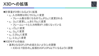
n426
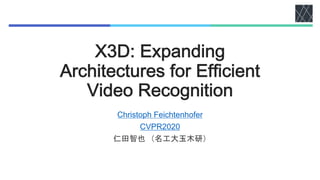
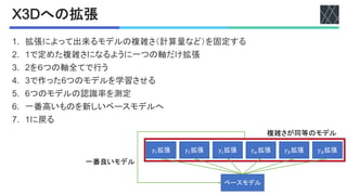
• ベースとなる26モデル
• 軸の探索をするモデル
• Tつの軸を全てCに設定
n426からTつの軸を探索
• フレームレート：𝛾!
• フレーム数：𝛾"
• 解像度：𝛾#
• チャネル幅：𝛾$
• ボトルネック幅：𝛾%
• 深さ：𝛾&
In relation to most of these works, our approach does
not assume a fixed inherited design from 2D networks, but
expands a tiny architecture across several axes in space, time,
channels and depth to achieve a good efficiency trade-off.
3. X3D Networks
Image classification architectures have gone through an
evolution of architecture design with progressively expand-
ng existing models along network depth [7,23,37,51,58,81],
nput resolution [27,57,60] or channel width [75,80]. Simi-
ar progress can be observed for the mobile image classifi-
cation domain where contracting modifications (shallower
networks, lower resolution, thinner layers, separable convo-
ution [24,25,29,48,82]) allowed operating at lower compu-
ational budget. Given this history in image ConvNet design,
a similar progress has not been observed for video architec-
ures as these were customarily based on direct temporal
extensions of image models. However, is single expansion
of a fixed 2D architecture to 3D ideal, or is it better to expand
stage filters output sizes T×S2
data layer stride γτ , 12
1γt×(112γs)2
conv1 1×32, 3×1, 24γw 1γt×(56γs)2
res2


1×12, 24γbγw
3×32, 24γbγw
1×12, 24γw

×γd 1γt×(28γs)2
res3


1×12, 48γbγw
3×32, 48γbγw
1×12, 48γw

×2γd 1γt×(14γs)2
res4


1×12, 96γbγw
3×32, 96γbγw
1×12, 96γw

×5γd 1γt×(7γs)2
res5


1×12, 192γbγw
3×32, 192γbγw
1×12, 192γw

×3γd 1γt×(4γs)2
conv5 1×12, 192γbγw 1γt×(4γs)2
pool5 1γt×(4γs)2 1×1×1
fc1 1×12, 2048 1×1×1
fc2 1×12, #classes 1×1×1
𝛾!が１なので!"

5. !$#への拡張
CU 拡張によって出来るモデルの複雑さ（計算量など）を固定する
2U Cで定めた複雑さになるように一つの軸だけ拡張
5U 2を６つの軸全てで行う
VU 5で作ったTつのモデルを学習させる
WU Tつのモデルの認識率を測定
TU 一番高いものを新しいベースモデルへ
DU Cに戻る
ベースモデル
𝛾!拡張 𝛾"拡張
𝛾#拡張 𝛾$拡張 𝛾%拡張 𝛾&拡張
一番良いモデル
複雑さが同等のモデル

6. !$#への拡張
τ
s
d
b
t
w
X3D
d
d
t
t
b
τ
τ
X3D-L
X3D-M
X3D-S
X3D-XS
s
s
s
X2D
w
X3D-XL
Model capacity in GFLOPs (# of multiply-adds x 109
)
0 5 15 25 35
10 20 30
80
75
70
65
60
55
50
Kinetics
top-1
accuracy
(%)
Figure 2. Progressive network expansion of X3D. The X2D base
model is expanded 1st
across bottleneck width (γb), 2nd
tempo-
ral resolution (γτ ), 3rd
spatial resolution (γs), 4th
depth (γd), 5th
model top-1 top-5
regime FLOPs Params
FLOPs (G) (G) (M)
X3D-XS 68.6 87.9 X-Small ≤ 0.6 0.60 3.76
X3D-S 72.9 90.5 Small ≤ 2 1.96 3.76
X3D-M 74.6 91.7 Medium ≤ 5 4.73 3.76
X3D-L 76.8 92.5 Large ≤ 20 18.37 6.08
X3D-XL 78.4 93.6 X-Large ≤ 40 35.84 11.0
Table 2. Expanded instances on K400-val. 10-Center clip testing is
used. We show top-1 and top-5 classification accuracy (%), as well
as computational complexity measured in GFLOPs (floating-point
operations, in # of multiply-adds ×109
) for a single clip input.
Inference-time computational cost is proportional to 10× of this,
as a fixed number of 10 of clips is used per video.
4.1. Expanded networks
The accuracy/complexity trade-off curve for the expan-
sion process on K400 is shown in Fig. 2. Expansion starts
from X2D that produces 47.75% top-1 accuracy (vertical
axis) with 1.63M parameters 20.67M FLOPs per clip (hori-
zontal axis), which is roughly doubled in each progressive
step. We use 10-Center clip testing as our default test setting
for expansion, so the overall cost per video is ×10. We
τ
s
d
b
t
w
X3D
d
d
t
t
b
τ
τ
X3D-L
X3D-M
X3D-S
X3D-XS
s
s
s
X2D
w
X3D-XL
Model capacity in GFLOPs (# of multiply-adds x 109
)
0 5 15 25 35
10 20 30
80
75
70
65
60
55
50
Kinetics
top-1
accuracy
(%)
Figure 2. Progressive network expansion of X3D. The X2D base
model is expanded 1st
across bottleneck width (γb), 2nd
tempo-
model top-1 top-5
regime FLOPs Params
FLOPs (G) (G) (M)
X3D-XS 68.6 87.9 X-Small ≤ 0.6 0.60 3.76
X3D-S 72.9 90.5 Small ≤ 2 1.96 3.76
X3D-M 74.6 91.7 Medium ≤ 5 4.73 3.76
X3D-L 76.8 92.5 Large ≤ 20 18.37 6.08
X3D-XL 78.4 93.6 X-Large ≤ 40 35.84 11.0
Table 2. Expanded instances on K400-val. 10-Center clip testing is
used. We show top-1 and top-5 classification accuracy (%), as well
as computational complexity measured in GFLOPs (floating-point
operations, in # of multiply-adds ×109
) for a single clip input.
Inference-time computational cost is proportional to 10× of this,
as a fixed number of 10 of clips is used per video.
4.1. Expanded networks
The accuracy/complexity trade-off curve for the expan-
sion process on K400 is shown in Fig. 2. Expansion starts
from X2D that produces 47.75% top-1 accuracy (vertical
axis) with 1.63M parameters 20.67M FLOPs per clip (hori-
zontal axis), which is roughly doubled in each progressive
step. We use 10-Center clip testing as our default test setting
!回目の拡張結果
𝛾!が一番良いモデル
一番良い結果となった拡張 拡張した結果から５つのモデルを抽出
拡張のコスト
• 456
• １ステップに６つのモデルを学習
• ６×ステップ数の学習
• K..$,$+-&:+&
• グリッドサーチ
• 全てのモデルを総当たり

7. 実験設定
nデータセット
• !"#$%"&'()**+,!-./0+-12"34*567
• !"#$%"&'(8**+,9-11$1"-/0+-12"34*5:7
• 9;-1-<$'+,=">?1<''@#/0+A99B4*587
n学習
• 554𝛾!× 554𝛾!にクロップ
• ランダムに反転
n推論
• 空間方向
• 554𝛾!× 554𝛾!にクロップ
• センタークロップ
• 空間軸にCクロップ
• 時間方向
• !個を一様にサンプリング

8. !$#性能比較
model pre top-1 top-5 test GFLOPs×views Param
I3D [6]
ImageNet
71.1 90.3 80.2 108 × N/A 12M
Two-Stream I3D [6] 75.7 92.0 82.8 216 × N/A 25M
Two-Stream S3D-G [76] 77.2 93.0 143 × N/A 23.1M
MF-Net [9] 72.8 90.4 11.1 × 50 8.0M
TSM R50 [41] 74.7 N/A 65 × 10 24.3M
Nonlocal R50 [68] 76.5 92.6 282 × 30 35.3M
Nonlocal R101 [68] 77.7 93.3 83.8 359 × 30 54.3M
Two-Stream I3D [6] - 71.6 90.0 216 × NA 25.0M
R(2+1)D [64] - 72.0 90.0 152 × 115 63.6M
Two-Stream R(2+1)D [64] - 73.9 90.9 304 × 115 127.2M
Oct-I3D + NL [8] - 75.7 N/A 28.9 × 30 33.6M
ip-CSN-152 [63] - 77.8 92.8 109 × 30 32.8M
SlowFast 4×16, R50 [14] - 75.6 92.1 36.1 × 30 34.4M
SlowFast 8×8, R101 [14] - 77.9 93.2 84.2 106 × 30 53.7M
SlowFast 8×8, R101+NL [14] - 78.7 93.5 84.9 116 × 30 59.9M
SlowFast 16×8, R101+NL [14] - 79.8 93.9 85.7 234 × 30 59.9M
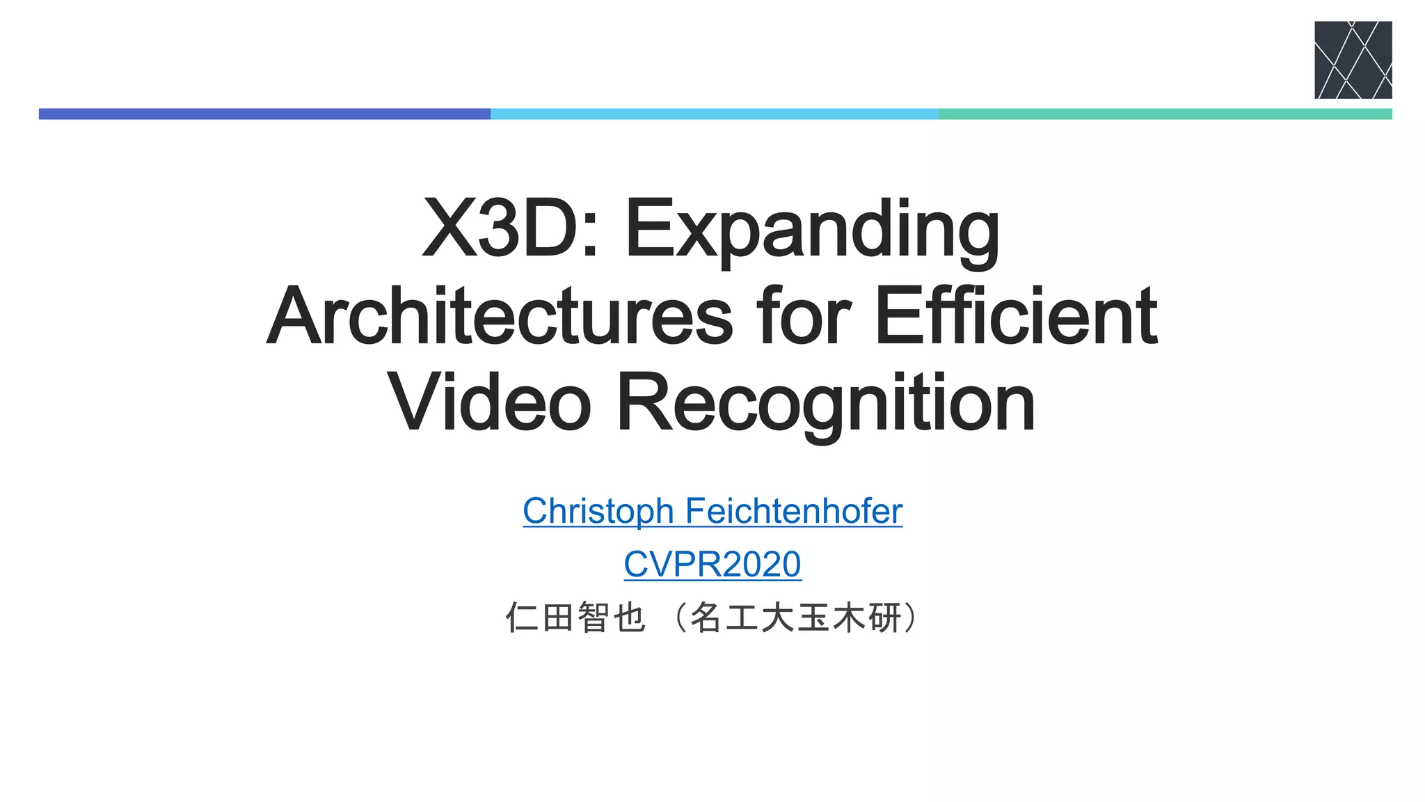
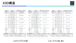
X3D-M - 76.0 92.3 82.9 6.2 × 30 3.8M
X3D-L - 77.5 92.9 83.8 24.8 × 30 6.1M
X3D-XL - 79.1 93.9 85.3 48.4 × 30 11.0M
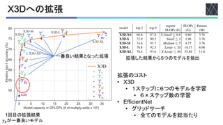
Table 4. Comparison to the state-of-the-art on K400-val & test.
We report the inference cost with a single “view" (temporal clip with
spatial crop) × the numbers of such views used (GFLOPs×views).
“N/A” indicates the numbers are not available for us. The “test”
model pretrain mAP GFLOPs×views Param
Nonlocal [68] ImageNet+Kinetics400 37.5 544 × 30 54.3M
STRG, +NL [69] ImageNet+Kinetics400 39.7 630 × 30 58.3M
Timeception [28] Kinetics-400 41.1 N/A×N/A N/A
LFB, +NL [71] Kinetics-400 42.5 529 × 30 122M
SlowFast, +NL [14] Kinetics-400 42.5 234 × 30 59.9M
SlowFast, +NL [14] Kinetics-600 45.2 234 × 30 59.9M
X3D-XL Kinetics-400 43.4 48.4 × 30 11.0M
X3D-XL Kinetics-600 47.1 48.4 × 30 11.0M
Table 6. Comparison with the state-of-the-art on Charades.
SlowFast variants are based on T×τ = 16×8.
model data top-1 top-5 FLOPs (G) Params (M)
EfficientNet3D-B0
K400
66.7 86.6 0.74 3.30
X3D-XS
val
68.6 (+1.9) 87.9 (+1.3) 0.60 (−1.4) 3.76 (+0.5)
EfficientNet3D-B3 72.4 89.6 6.91 8.19
X3D-M 74.6 (+2.2) 91.7 (+2.1) 4.73 (−2.2) 3.76 (−4.4)
EfficientNet3D-B4 74.5 90.6 23.80 12.16
X3D-L 76.8 (+2.3) 92.5 (+1.9) 18.37 (−5.4) 6.08 (−6.1)
EfficientNet3D-B0
K400
64.8 85.4 0.74 3.30
X3D-XS
test
66.6 (+1.8) 86.8 (+1.4) 0.60 (−1.4) 3.76 (+0.5)
EfficientNet3D-B3 69.9 88.1 6.91 8.19
X3D-M 73.0 (+2.1) 90.8 (+2.7) 4.73 (−2.2) 3.76 (−4.4)
EfficientNet3D-B4 71.8 88.9 23.80 12.16
X3D-XL - 79.1 93.9 85.3 48.4 × 30 11.0M
Table 4. Comparison to the state-of-the-art on K400-val & test.
We report the inference cost with a single “view" (temporal clip with
spatial crop) × the numbers of such views used (GFLOPs×views).
“N/A” indicates the numbers are not available for us. The “test”
column shows average of top1 and top5 on the Kinetics-400 testset.
model pretrain top-1 top-5 GFLOPs×views Param
I3D [3] - 71.9 90.1 108 × N/A 12M
Oct-I3D + NL [8] ImageNet 76.0 N/A 25.6 × 30 12M
SlowFast 4×16, R50 [14] - 78.8 94.0 36.1 × 30 34.4M
SlowFast 16×8, R101+NL [14] - 81.8 95.1 234 × 30 59.9M
X3D-M - 78.8 94.5 6.2 × 30 3.8M
X3D-XL - 81.9 95.5 48.4 × 30 11.0M
Table 5. Comparison with the state-of-the-art on Kinetics-600.
Results are consistent with K400 in Table 4 above.
Kinetics-600 is a larger version of Kinetics that shall
demonstrate further generalization of our approach. Re-
sults are shown in Table 5. Our variants demonstrate similar
performance as above, with the best model now providing
slightly better performance than the previous state-of-the-
art SlowFast 16×8, R101+NL [14], again for 4.8× fewer
FLOPs (i.e. multiply-add operations) and 5.5× fewer param-
eter. In the lower computation regime, X3D-M is compara-
ble to SlowFast 4×16, R50 but requires 5.8× fewer FLOPs
and 9.1× fewer parameters.
Charades [49] is a dataset with longer range activities. Ta-
model pre top-1 top-5 test GFLOPs×views Param
I3D [6]
ImageNet
71.1 90.3 80.2 108 × N/A 12M
Two-Stream I3D [6] 75.7 92.0 82.8 216 × N/A 25M
Two-Stream S3D-G [76] 77.2 93.0 143 × N/A 23.1M
MF-Net [9] 72.8 90.4 11.1 × 50 8.0M
TSM R50 [41] 74.7 N/A 65 × 10 24.3M
Nonlocal R50 [68] 76.5 92.6 282 × 30 35.3M
Nonlocal R101 [68] 77.7 93.3 83.8 359 × 30 54.3M
Two-Stream I3D [6] - 71.6 90.0 216 × NA 25.0M
R(2+1)D [64] - 72.0 90.0 152 × 115 63.6M
Two-Stream R(2+1)D [64] - 73.9 90.9 304 × 115 127.2M
Oct-I3D + NL [8] - 75.7 N/A 28.9 × 30 33.6M
ip-CSN-152 [63] - 77.8 92.8 109 × 30 32.8M
SlowFast 4×16, R50 [14] - 75.6 92.1 36.1 × 30 34.4M
SlowFast 8×8, R101 [14] - 77.9 93.2 84.2 106 × 30 53.7M
SlowFast 8×8, R101+NL [14] - 78.7 93.5 84.9 116 × 30 59.9M
model pretrain mAP GFLOPs×views Param
Nonlocal [68] ImageNet+Kinetics400 37.5 544 × 30 54.3M
STRG, +NL [69] ImageNet+Kinetics400 39.7 630 × 30 58.3M
Timeception [28] Kinetics-400 41.1 N/A×N/A N/A
LFB, +NL [71] Kinetics-400 42.5 529 × 30 122M
SlowFast, +NL [14] Kinetics-400 42.5 234 × 30 59.9M
SlowFast, +NL [14] Kinetics-600 45.2 234 × 30 59.9M
X3D-XL Kinetics-400 43.4 48.4 × 30 11.0M
X3D-XL Kinetics-600 47.1 48.4 × 30 11.0M
Table 6. Comparison with the state-of-the-art on Charades.
SlowFast variants are based on T×τ = 16×8.
model data top-1 top-5 FLOPs (G) Params (M)
EfficientNet3D-B0 66.7 86.6 0.74 3.30
"#$%&#'()*++
"#$%&#'(),++
-./0/1%(
事前
学習
既存
手法
同等の性能よりも
計算量削減

9. !$#性能比較
SlowFast, +NL [14] Kinetics-600 45.2 234 × 30 59.9M
X3D-XL Kinetics-400 43.4 48.4 × 30 11.0M
X3D-XL Kinetics-600 47.1 48.4 × 30 11.0M
Table 6. Comparison with the state-of-the-art on Charades.
SlowFast variants are based on T×τ = 16×8.
model data top-1 top-5 FLOPs (G) Params (M)
EfficientNet3D-B0
K400
66.7 86.6 0.74 3.30
X3D-XS
val
68.6 (+1.9) 87.9 (+1.3) 0.60 (−1.4) 3.76 (+0.5)
EfficientNet3D-B3 72.4 89.6 6.91 8.19
X3D-M 74.6 (+2.2) 91.7 (+2.1) 4.73 (−2.2) 3.76 (−4.4)
EfficientNet3D-B4 74.5 90.6 23.80 12.16
X3D-L 76.8 (+2.3) 92.5 (+1.9) 18.37 (−5.4) 6.08 (−6.1)
EfficientNet3D-B0
K400
64.8 85.4 0.74 3.30
X3D-XS
test
66.6 (+1.8) 86.8 (+1.4) 0.60 (−1.4) 3.76 (+0.5)
EfficientNet3D-B3 69.9 88.1 6.91 8.19
X3D-M 73.0 (+2.1) 90.8 (+2.7) 4.73 (−2.2) 3.76 (−4.4)
EfficientNet3D-B4 71.8 88.9 23.80 12.16
X3D-L 74.6 (+2.8) 91.4 (+2.5) 18.37 (−5.4) 6.08 (−6.1)
Table 7. Comparison to EfficientNet3D: We compare to a 3D
version of EfficientNet on K400-val and test. 10-Center clip testing
is used. EfficientNet3D has the same mobile components as X3D.
but was found by searching a large number of models for op-
timal trade-off on image-classification. This ablation studies
if a direct extension of EfficientNet to 3D is comparable to
X3D (which is expanded by only training few models). Effi-
cientNet models are provided for various complexity ranges.
233#'#%$&4%&56との比較
456のハイパーパラメータ探索が優れている
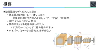
Inference cost per video in TFLOPs (# of multiply-adds x 1012
)
0.0 0.2 0.4 0.6 0.8
76
74
72
70
68
66
64
Kinetics
top-1
accuracy
(%)
78
SlowFast 8x8, R101+NL
SlowFast 8x8, R101
X3D-XL
X3D-M
X3D-S
CSN (Channel-Separated Networks)
TSM (Temporal Shift Module)
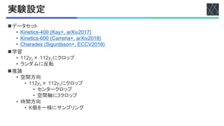
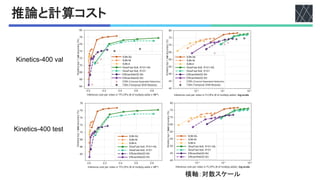
Figure 3. Accuracy/complexity trade-off on Kinetics-400 for dif-
ferent number of inference clips per video. The top-1 accuracy
(vertical axis) is obtained by K-Center clip testing where the num-
ber of temporal clips K ∈ {1, 3, 5, 7, 10} is shown in each curve.
The horizontal axis shows the full inference cost per video.
Inference cost. In many cases, like the experiments before,
推論時のクリップ数と認識率
!75クリップの
比較
5クリップ以上は
計算量に対して認識率の伸びが悪い

10. まとめ
nTつのハイパーパラメータを探索してできたモデル
• 探索にかかるコストが少ない
n計算量と性能の効率を重視したモデル
• 同等の性能のモデルと比べて軽い
n推論時の計算量
• 精度を重要視しないならクリップ数を多くする必要がない

11. 補足スライド

12. !$#への拡張
n𝑋 = 𝑎𝑟𝑔𝑚𝑎𝑥(,* ( +, 𝐽(𝑍)
• 𝑋:探索する軸{𝛾!, 𝛾", 𝛾#, 𝛾$, 𝛾%, 𝛾&}
• 𝐽 𝑋 ：ネットワークの精度を表す関数
• 𝐶(𝑋)：ネットワークの複雑性を表す関数
• 演算回数 （実験で使用）
• ランタイム
• パラメータ
• メモリ
• ,X目標とする複雑さ

13. !$#への拡張
n計算量が２倍になるように拡張
• 𝛾!：入力時間は同じで3UW𝛾!に変更
• フレーム数は倍になるので𝛾"が2𝛾"に変更される
• 𝛾"： 2𝛾"に変更し、𝛾!を3UDW𝛾!に変更
• フレームレートと入力時間がCUW倍になっている
• 𝛾#： 2𝛾#に変更
• 𝛾$：2𝛾$に変更
• 𝛾%：2U2W𝛾%に変更
• 𝛾&：2U2𝛾&に変更
n456モデルの抽出
• 基準となるY*NZ0%を超えないように𝛾を調整
• 456FJX７回目の𝛾"拡張を2Y*NZ0%以下になるように調整

14. !$#構造
stage filters output sizes T×H×W
data layer stride 6, 12
13×160×160
conv1 1×32, 3×1, 24 13×80×80
res2


1×12, 54
3×32, 54
1×12, 24

×3 13×40×40
res3


1×12, 108
3×32, 108
1×12, 48

×5 13×20×20
res4


1×12, 216
3×32, 216
1×12, 96

×11 13×10×10
res5


1×12, 432
3×32, 432
1×12, 192

×7 13×5×5
conv5 1×12, 432 13×5×5
pool5 13×5×5 1×1×1
fc1 1×12, 2048 1×1×1
fc2 1×12, #classes 1×1×1
(a) X3D-S with 1.96G FLOPs, 3.76M param, and
72.9% top-1 accuracy using expansion of γτ = 6,
γt= 13, γs=
√
2, γw= 1, γb= 2.25, γd= 2.2.
stage filters output sizes T×H×W
data layer stride 5, 12
16×224×224
conv1 1×32, 3×1, 24 16×112×112
res2


1×12, 54
3×32, 54
1×12, 24

×3 16×56×56
res3


1×12, 108
3×32, 108
1×12, 48

×5 16×28×28
res4


1×12, 216
3×32, 216
1×12, 96

×11 16×14×14
res5


1×12, 432
3×32, 432
1×12, 192

×7 16×7×7
conv5 1×12, 432 16×7×7
pool5 16×7×7 1×1×1
fc1 1×12, 2048 1×1×1
fc2 1×12, #classes 1×1×1
(b) X3D-M with 4.73G FLOPs, 3.76M param, and
74.6% top-1 accuracy using expansion of γτ = 5,
γt= 16, γs= 2, γw= 1, γb= 2.25, γd= 2.2.
stage filters output sizes T×H×W
data layer stride 5, 12
16×312×312
conv1 1×32, 3×1, 32 16×156×156
res2


1×12, 72
3×32, 72
1×12, 32

×5 16×78×78
res3


1×12, 162
3×32, 162
1×12, 72

×10 16×39×39
res4


1×12, 306
3×32, 306
1×12, 136

×25 16×20×20
res5


1×12, 630
3×32, 630
1×12, 280

×15 16×10×10
conv5 1×12, 630 16×10×10
pool5 16×10×10 1×1×1
fc1 1×12, 2048 1×1×1
fc2 1×12, #classes 1×1×1
(c) X3D-XL with 35.84G FLOPs & 10.99M param,
and 78.4% top-1 acc. using expansion of γτ = 5,
γt= 16, γs= 2
√
2, γw= 2.9, γb= 2.25, γd= 5.
Table 3. Three instantiations of X3D with varying complexity. The top-1 accuracy corresponds to 10-Center view testing on K400. The
models in (a) and (b) only differ in spatiotemporal resolution of the input and activations (γt, γτ , γs), and (c) differs from (b) in spatial
resolution, γs, width, γw, and depth, γd. See Table 1 for X2D. Surprisingly X3D-XL has a maximum width of 630 feature channels.
入力サイズだけが違う 入力、チャネル数、深さ

15. 学習 %&'()*'+,-.//0
nバッチサイズ：C32V
• Y0[１台につき８クリップ
• クリップでバッチノーマライゼーショ
ン
n反復数：2WTエポック
nオプティマイザー：JY6
• S'S+-&GSX3UI
• =+$]"&)?+,>^X5×10-.
• 学習率XCUT
nドロップアウト：3UW
nスケジューラ
• 最初の333反復
• 線形ウォームアップ
• コサインスケジューラ
• 𝜂 8 0.5 cos
/
/!"#
𝜋 + 1
• 𝜂：CUT
• 𝑛012：最大学習反復数

16. 学習
nO$-+&$,%FT33
• 反復数：O$-+&$,%FV33の倍
• スケジューラも同様に倍
n!">#>?+%
• O$-+&$,%のモデルをファインチューニ
ング
• バッチサイズ：CT
• 学習率：3U32
• =+$]"&)?+,>^：10-.
• 入力のフレームレートを半分
• 長い時間を推論するため
n_/_
• 反復数：Tエポック
• 最初のC333反復
• 線形ウォームアップ
• LZ[閾値：3UI

17. !$#性能比較 （アクション検出）
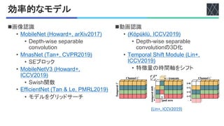
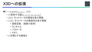
nデータセット
• _/_);YG@A)!/0123CE
n推論
• C28𝛾#×C2𝛾#にセンタークロップ
XL
M
S
model AVA pre val mAP GFLOPs Param
LFB, R50+NL [71]
v2.1 K400
25.8 529 73.6M
LFB, R101+NL [71] 26.8 677 122M
X3D-XL 26.1 48.4 11.0M
SlowFast 4×16, R50 [14]
v2.2 K600
24.7 52.5 33.7M
SlowFast, 8×8 R101+NL [14] 27.4 146 59.2M
X3D-M 23.2 6.2 3.1M
X3D-XL 27.4 48.4 11.0M
Table 8. Comparison with the state-of-the-art on AVA. All meth-
ods use single center crop inference; full testing cost is directly

18. 推論と計算コスト
Inference cost per video in TFLOPs (# of multiply-adds x 1012
)
0.0 0.2 0.4 0.6 0.8
76
74
72
70
68
66
64
Kinetics
top-1
val
accuracy
(%)
78
80
SlowFast 8x8, R101+NL
SlowFast 8x8, R101
X3D-XL
X3D-M
EfficientNet3D-B4
EfficientNet3D-B3
X3D-S
CSN (Channel-Separated Networks)
TSM (Temporal Shift Module)
Inference cost per video in FLOPs (# of multiply-adds), log-scale
SlowFast 8x8, R101+NL
SlowFast 8x8, R101
X3D-XL
X3D-M
EfficientNet3D-B4
EfficientNet3D-B3
X3D-S
CSN (Channel-Separated Networks)
TSM (Temporal Shift Module)
75
70
65
60
55
50
45
Kinetics
top-1
val
accuracy
(%)
80
40
1010
1011
1012
76
74
72
70
68
66
64
Kinetics
top-1
test
accuracy
(%)
78
Inference cost per video in TFLOPs (# of multiply-adds x 1012
)
0.0 0.2 0.4 0.6 0.8
SlowFast 8x8, R101+NL
SlowFast 8x8, R101
X3D-XL
X3D-M
EfficientNet3D-B4
EfficientNet3D-B3
X3D-S
SlowFast 8x8, R101+NL
SlowFast 8x8, R101
X3D-XL
X3D-M
EfficientNet3D-B4
EfficientNet3D-B3
X3D-S
75
70
65
60
55
50
45
Kinetics
top-1
test
accuracy
(%)
80
40
Inference cost per video in FLOPs (# of multiply-adds), log-scale
1010
1011
1012
Figure A.1. Accuracy/complexity trade-off on K400-val (top) & test (bottom) for varying # of inference clips per video. The top-1
accuracy (vertical axis) is obtained by K-Center clip testing where the number of temporal clips K 2 {1, 3, 5, 7, 10} is shown in each curve.
"#$%&#'()*++89/:
"#$%&#'()*++8&%(&
横軸：対数スケール

19. 追加実験
n6+(&"F=$%+)%+(>#>89+),'-B'9G&$'-
• 通常の56畳み込みに変更し𝛾%を変更
• パラメータ数が同等になるように
• 通常の56畳み込みに変更
nJ=$%"
• 1+N[に変更で性能が少し低下
• メモリを優先するなら1+N[
nJKブロック
• 削除で性能低下
• パフォーマンスに大きな影響を与えている
model top-1 top-5 FLOPs (G) Param (M)
X3D-S 72.9 90.5 1.96 3.76
CW conv b= 0.6 68.9 88.8 1.95 3.16
CW conv 73.2 90.4 17.6 22.1
swish 72.0 90.4 1.96 3.76
SE 71.3 89.9 1.96 3.60
(a) Ablating mobile components on a Small model.
X3D
C
Table A.1. Ablations of mobile components for video classification on K
parameters, and computational complexity measured in GFLOPs (floatin
input of size t⇥112 s⇥112 x. Inference-time computational cost is repo
The results show that removing channel-wise separable convolution (CW
increases mutliply-adds and parameters at slightly higher accuracy, while
[5] Ross Girshick, Ilija Radosavovic, Georgia Gkioxari, Piotr
Dollár, and Kaiming He. Detectron. https://github.
com/facebookresearch/detectron, 2018. 1
[6] Priya Goyal, Piotr Dollár, Ross Girshick, Pieter Noord-
huis, Lukasz Wesolowski, Aapo Kyrola, Andrew Tulloch,
Yangqing Jia, and Kaiming He. Accurate, large minibatch
SGD: training ImageNet in 1 hour. arXiv:1706.02677, 2017.
1
[7] Chunhui Gu, Chen Sun, David A. Ross, Carl Vondrick, Car-
oline Pantofaru, Yeqing Li, Sudheendra Vijayanarasimhan,
George Toderici, Susanna Ricco, Rahul Sukthankar, Cordelia
[1
[1
[1
model top-1 top-5 FLOPs (G) Param (M)
X3D-S 72.9 90.5 1.96 3.76
CW conv b= 0.6 68.9 88.8 1.95 3.16
CW conv 73.2 90.4 17.6 22.1
swish 72.0 90.4 1.96 3.76
SE 71.3 89.9 1.96 3.60
(a) Ablating mobile components on a Small model.
model top-1 top-5 FLOPs (G) Param (M)
X3D-XL 78.4 93.6 35.84 11.0
CW conv, b= 0.56 76.0 92.6 34.80 9.73
CW conv 79.2 93.5 365.4 95.1
swish 78.0 93.4 35.84 11.0
SE 77.1 93.0 35.84 10.4
(b) Ablating mobile components on an X-Large model.
Table A.1. Ablations of mobile components for video classification on K400-val. We show top-1 and top-5 classification accuracy (%
parameters, and computational complexity measured in GFLOPs (floating-point operations, in # of multiply-adds ⇥109
) for a single c
input of size t⇥112 s⇥112 x. Inference-time computational cost is reported GFLOPs ⇥10, as a fixed number of 10-Center views is us
The results show that removing channel-wise separable convolution (CW conv) with unchanged bottleneck expansion ratio, b, drastica
increases mutliply-adds and parameters at slightly higher accuracy, while swish has a smaller effect on performance than SE.
[5] Ross Girshick, Ilija Radosavovic, Georgia Gkioxari, Piotr
Dollár, and Kaiming He. Detectron. https://github.
com/facebookresearch/detectron, 2018. 1
quality estimation of multiple intermediate frames for vid
interpolation. In Proc. CVPR, 2018. 1
[17] Alex Krizhevsky, Ilya Sutskever, and Geoffrey E Hinton. Im