Jaejun Yoo, Namhyuk Ahn, Kyung-Ah Sohn; Rethinking Data Augmentation for Image Super-resolution: A Comprehensive Analysis and a New Strategy, Proceedings of the IEEE/CVF Conference on Computer Vision and Pattern Recognition (CVPR), 2020, pp. 8375-8384 https://openaccess.thecvf.com/content_CVPR_2020/html/Yoo_Rethinking_Data_Augmentation_for_Image_Super-resolution_A_Comprehensive_Analysis_and_CVPR_2020_paper.html

1. !"#$%&'%&()*+#+),-(."&#+#%/&)0/1)
2.+(")3-4"151"6/7-#%/&8
,)9/.41"$"&6%:"),&+7;6%6)+&<)
+)=">)3#1+#"(;
!"#$%&'())*'+",-.%/'0-&*'1.%&230-'4)-&*'56789:9:
木全潤（名工大玉木研）
論文紹介9:9;<;9<;=

2. 概要
nデータ拡張 >?0@
• 学習データの分布を広げることで追加の計算コストをかけずに性能向上
• 高レベル（分類など）のタスクで盛んに研究
n超解像 >48@
• 画像の解像度を復元する
• ほとんどが合成データセットに依存
• ?0の研究はほとんどされていない
nやったこと
• 高レベルタスク用の?0手法の48に対する効果の包括的な分析
• 48用の?0手法5%ABC%Dの提案

3. !"#$%&'"($
!"手法
n画素空間における?0手法
• 0%A)'0%2,#&A'EF/G&H*'
56789:;IJ
• ?0の最適なパラメータを探索
• KGL%M'EN-"&2H*'"DOGP9:;QJ
• 5%A)%A'E?#6DG#RH*'"DOGP9:;QJ
• 5%AKGL'E(%&H*'S5569:;IJ
esolution (b) Low resolution (c) CutBlur (d) Schematic illustration of CutBlur operation
ow resolution (c) CutBlur (d) Schematic illustration of CutBlur operation
GB permute (g) Cutout (25%) [7] (h) Mixup [30] (i) CutMix [29] (j) CutMixup
ethods. (Top) An illustrative example of our proposed method, CutBlur. CutBlur generates an augmented
ow resolution (LR) input image onto the ground-truth high resolution (HR) image region and vice versa
e examples of the existing augmentation techniques and a new variation of CutMix and Mixup, CutMixup.
rresponding ground-truth high 2. Data augmentation analysis
(a) High resolution (b) Low resolution (c) CutBlur (d) Schematic illustration of CutBlur operation
(e) Blend (f) RGB permute (g) Cutout (25%) [7] (h) Mixup [30] (i) CutMix [29] (j) CutMixup
Figure 1. Data augmentation methods. (Top) An illustrative example of our proposed method, CutBlur. CutBlur generates an augmented
image by cut-and-pasting the low resolution (LR) input image onto the ground-truth high resolution (HR) image region and vice versa
(Section 3). (Bottom) Illustrative examples of the existing augmentation techniques and a new variation of CutMix and Mixup, CutMixup.
(LR) image patch into its corresponding ground-truth high 2. Data augmentation analysis
(a) High resolution (b) Low resolution (c) CutBlur (d) Schematic illustration of CutBlur operation
(e) Blend (f) RGB permute (g) Cutout (25%) [7] (h) Mixup [30] (i) CutMix [29] (j) CutMixup
ure 1. Data augmentation methods. (Top) An illustrative example of our proposed method, CutBlur. CutBlur generates an augmented
age by cut-and-pasting the low resolution (LR) input image onto the ground-truth high resolution (HR) image region and vice versa
ction 3). (Bottom) Illustrative examples of the existing augmentation techniques and a new variation of CutMix and Mixup, CutMixup.
R) image patch into its corresponding ground-truth high 2. Data augmentation analysis
n特徴量空間における?0手法
• T#"A%D#',GLG&2
• K"&GU)CV'KGL%M'E6#D,"H*'
7KW89:;IJなど
• 特徴量を混合
• 4-"/G&2
• 4-"/#34-"/#'EX"RA"CVGH*'
"DOGP9:;QJ*'4-"/#?D)M
E(","V"H*'"DOGP9:;YJ
• 特長量を確率的アフィン変換
• ?D)MMG&2
• ?D)M)%A'E4DGP"RA"P"H*'
!KW89:;ZJ関連の手法
• 特長量を欠落
)*+,*+
-&.*/ )*+-&.

4. #$での効果の検証
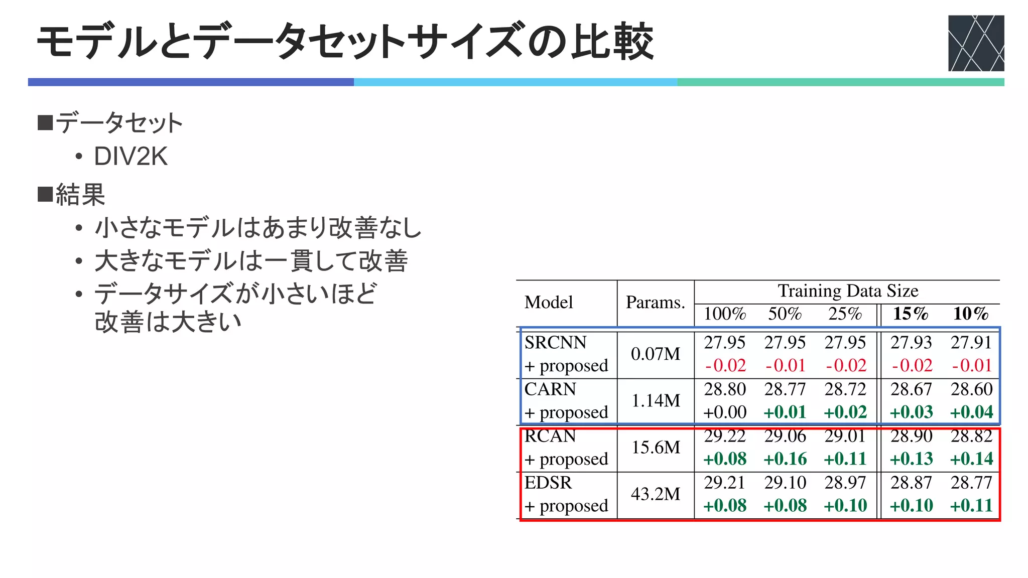
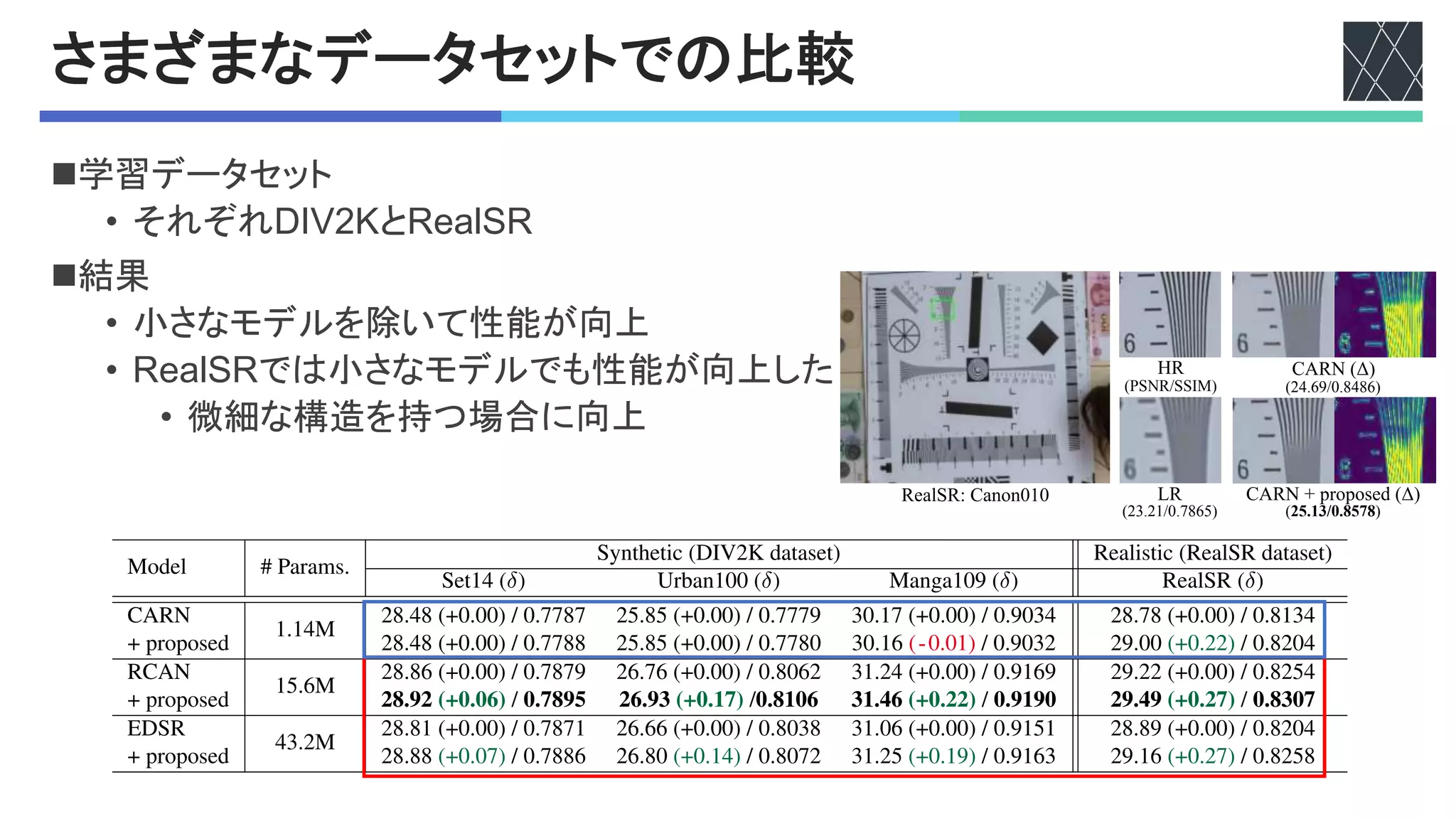
n結果
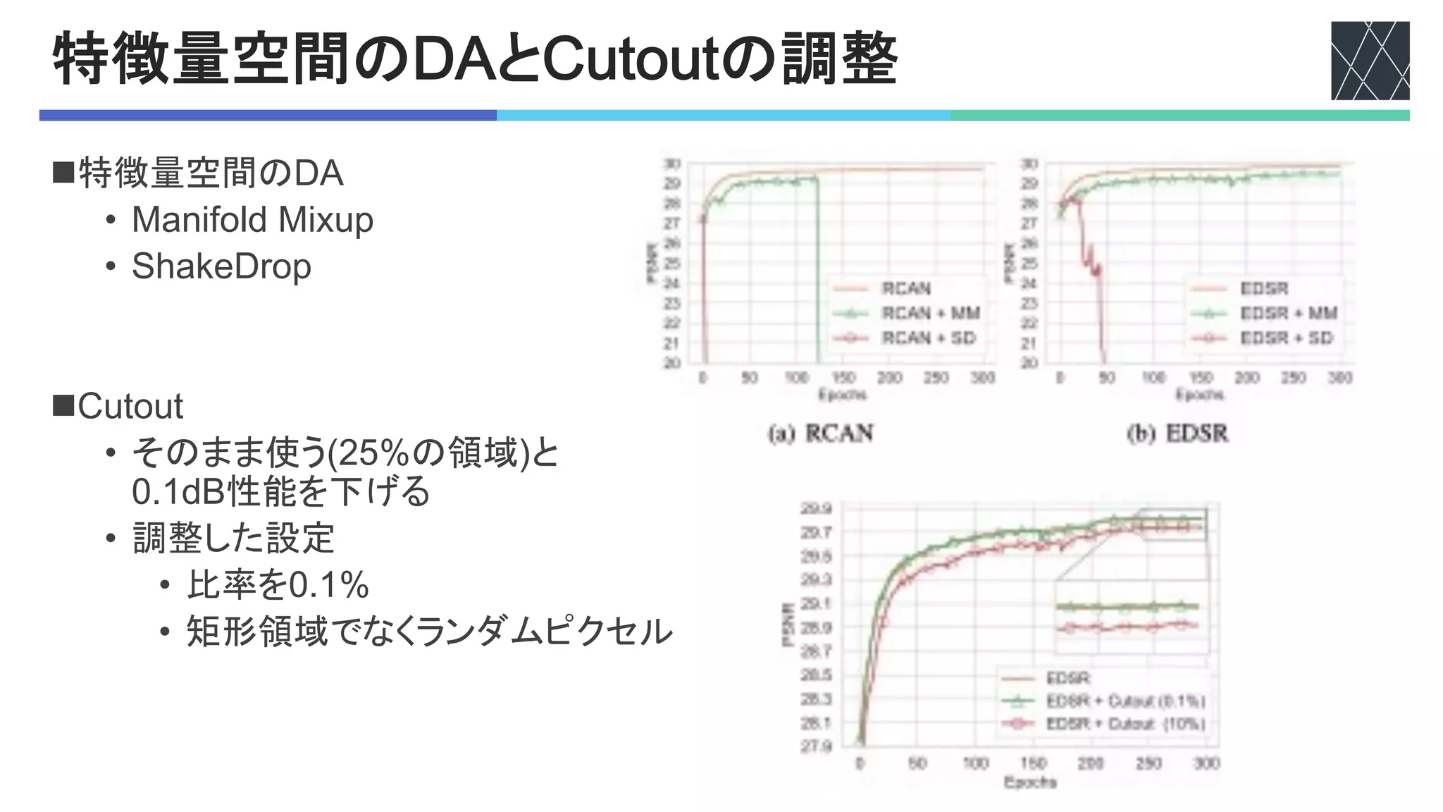
• 画素空間の?0は設定に注意すれば少し有効
• 特長空間の?0では性能低下
• 空間情報が失われるため
n分析
• 画像に構造的な変化を与えない?0が有効？
• テスト項目を追加
• 5%AKGL%M
• 5%AKGLとKGL%Mを合わせる
• 8XB'M#D,%A"AG)&
• BC#&V
(a) High resolution (b
(e) Blend (
Figure 1. Data augmentation
image by cut-and-pasting th
(a) High resolution (b) Low resolution (c) CutBlur
(e) Blend (f) RGB permute (g) Cutout (25%) [7] (h) Mix
Figure 1. Data augmentation methods. (Top) An illustrative example of our pro
image by cut-and-pasting the low resolution (LR) input image onto the ground
) Low resolution (c) CutBlur (d) Schematic illustration of CutBlur operation
) RGB permute (g) Cutout (25%) [7] (h) Mixup [30] (i) CutMix [29] (j) CutMixup
methods. (Top) An illustrative example of our proposed method, CutBlur. CutBlur generates an augmented
e low resolution (LR) input image onto the ground-truth high resolution (HR) image region and vice versa
2.2. Analysis of existing DA methods
The core idea of many augmentation methods is to
partially block or confuse the training signal so that the
model acquires more generalization power. However, unlike
the high-level tasks, such as classification, where a model
should learn to abstract an image, the local and global re-
lationships among pixels are especially more important in
the low-level vision tasks, such as denoising and super-
resolution. Considering this characteristic, it is unsurprising
that DA methods, which lose the spatial information, limit
the model’s ability to restore an image. Indeed, we observe
that the methods dropping the information [5, 11, 25] are
detrimental to the SR performance and especially harmful
in the feature space, which has larger receptive fields. Every
feature augmentation method significantly drops the perfor-
mance. Here, we put off the results of every DA method that
degrades the performance in the supplementary material.
On the other hand, DA methods in pixel space bring
some improvements when applied carefully (Table 1)1
. For
example, Cutout [7] with default setting (dropping 25%
of pixels in a rectangular shape) significantly degrades the
original performance by 0.1 dB. However, we find that
Cutout gives a positive effect (DIV2K: +0.01 dB and Re-
alSR: +0.06 dB) when applied with 0.1% ratio and erasing
random pixels instead of a rectangular region. Note that this
Table 1. PSNR (dB) comparison of different data augmentation
methods in super-resolution. We report the baseline model (EDSR
[15]) performance that is trained on DIV2K (×4) [2] and RealSR
(×4) [4]. The models are trained from scratch. δ denotes the per-
formance gap between with and without augmentation.
Method DIV2K (δ) RealSR (δ)
EDSR 29.21 (+0.00) 28.89 (+0.00)
Cutout [7] (0.1%) 29.22 (+0.01) 28.95 (+0.06)
CutMix [29] 29.22 (+0.01) 28.89 (+0.00)
Mixup [30] 29.26 (+0.05) 28.98 (+0.09)
CutMixup 29.27 (+0.06) 29.03 (+0.14)
RGB perm. 29.30 (+0.09) 29.02 (+0.13)
Blend 29.23 (+0.02) 29.03 (+0.14)
CutBlur 29.26 (+0.05) 29.12 (+0.23)
All DA’s (random) 29.30 (+0.09) 29.16 (+0.27)
3. CutBlur
In this section, we describe the CutBlur, a new augmen-
tation method that is designed for the super-resolution task.
3.1. Algorithm
Let xLR ∈ RW ×H×C
and xHR ∈ RsW ×sH×C
are LR
and HR image patches and s denotes a scale factor in the
)*+-&.*/ 01!%/$2' !3$45

5. %&'()&*
n低解像度画像 >W8@と高解像度画像 >[8@を合成
• W8をアップサンプリング
• [8と同じ解像度まで
• BG%]G'/#D&#Cを使用
• どちらかの一部をもう片方に合成
n特徴
• 大きな情報の損失や
構造の変化がない
• 「どこ」で「どのくらい」超解像
するかを学習
• ランダムな[8比率や
位置によって正則化
(a) High resolution (b) Low resolution (c) CutBlur
(a) High resolution (b) Low resolution (c) CutBlur (d) Schematic illustration of CutBl
(a) High resolution (b) Low resolution (c) CutBlur
(a) High resolution (b) Low resolution (c) CutBlur (d) Schematic illustration of CutBlur operation
(e) Blend (f) RGB permute (g) Cutout (25%) [7] (h) Mixup [30] (i) CutMix [29] (j) CutMixup
Figure 1. Data augmentation methods. (Top) An illustrative example of our proposed method, CutBlur. CutBlur generates an augmented
image by cut-and-pasting the low resolution (LR) input image onto the ground-truth high resolution (HR) image region and vice versa

6. 実験設定
n48モデル
• 小さなモデル
• 485++'E?)&2H*'70KS9:;^J
• 508+'E0-&H*'F5569:;YJ
• 大きなモデル
• 850+'EN-"&2H*'F5569:;YJ
• F?48'EWG,H*'5678_9:;QJ
n拡張の適用確率M
• 小さなモデル
• :`9
• 大きなモデル
• ;`:
nデータセット
• 学習画像
• 合成データセット
• !"#$%&'()*+,-./0&1#234$5678
• 実画像データセット
• 3.9:;3&'19)/0&9<=)>$56?8
• 評価画像
• 合成画像
• ;.-6@&'A9BC/0&"DDD$5658
• E<F9B655&'GH9BC/0&1#23$56I8
• J9BC965?&'J9-KH)/0&9<=)>$56I8
• 実画像
• 3.9:;3のテスト画像

7. +,"の説明と既存!"との比較
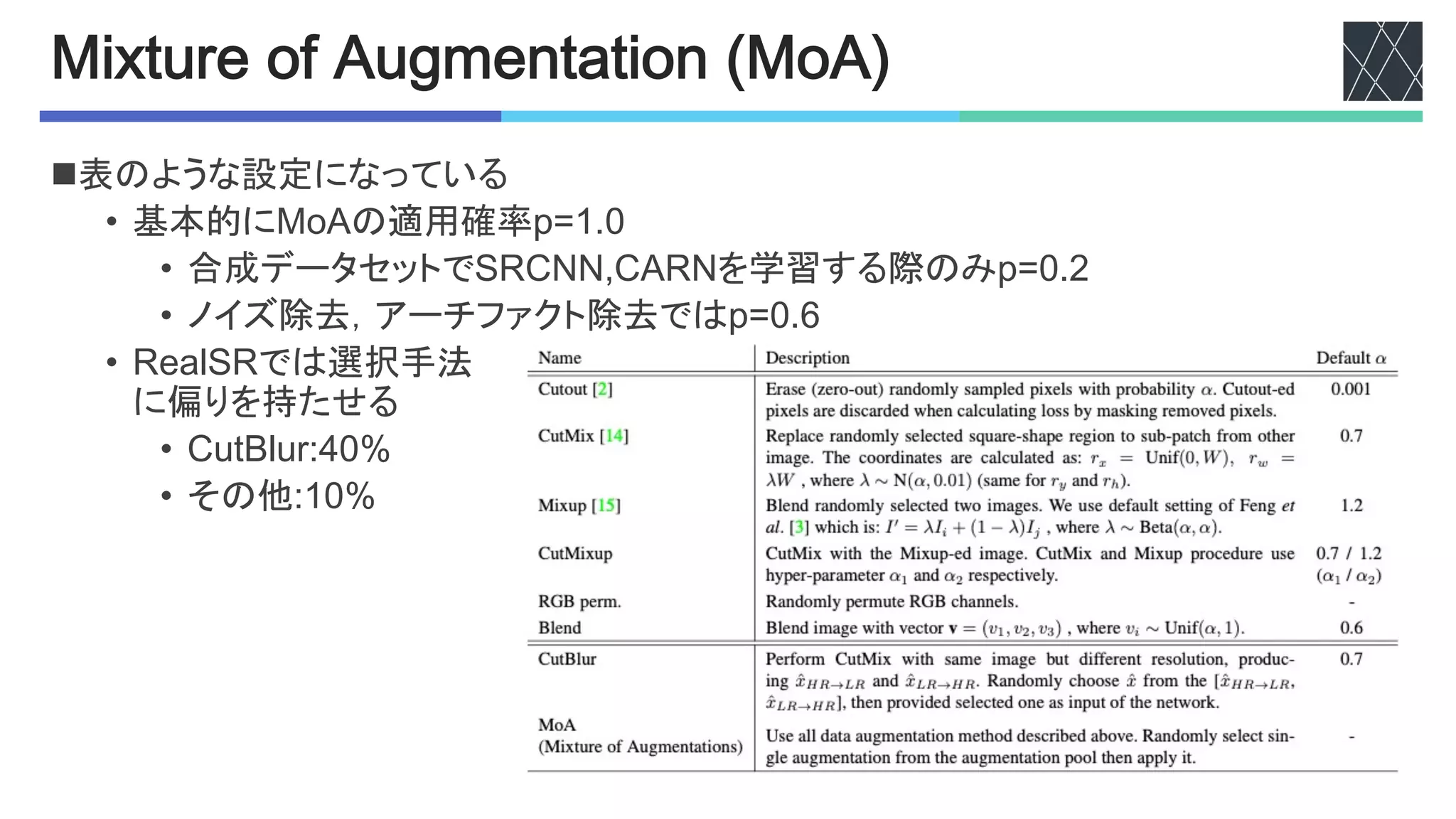
nKGLA%D#')U'"%2,#&A"AG)&'>K)0@
• さまざまな?0を統合
• 確率Mで?0するかを決定
• ?0するならランダムに選択
n比較結果
• 追加した項目は効果があった
• 5%ABC%Dでより良い結果
• K)0で最も良い結果
• 実画像データセットの方が
恩恵が大きい
nalysis of existing DA methods
core idea of many augmentation methods is to
y block or confuse the training signal so that the
acquires more generalization power. However, unlike
h-level tasks, such as classification, where a model
learn to abstract an image, the local and global re-
hips among pixels are especially more important in
w-level vision tasks, such as denoising and super-
on. Considering this characteristic, it is unsurprising
A methods, which lose the spatial information, limit
del’s ability to restore an image. Indeed, we observe
methods dropping the information [5, 11, 25] are
ntal to the SR performance and especially harmful
eature space, which has larger receptive fields. Every
augmentation method significantly drops the perfor-
Here, we put off the results of every DA method that
es the performance in the supplementary material.
Table 1. PSNR (dB) comparison of different data augmentation
methods in super-resolution. We report the baseline model (EDSR
[15]) performance that is trained on DIV2K (×4) [2] and RealSR
(×4) [4]. The models are trained from scratch. δ denotes the per-
formance gap between with and without augmentation.
Method DIV2K (δ) RealSR (δ)
EDSR 29.21 (+0.00) 28.89 (+0.00)
Cutout [7] (0.1%) 29.22 (+0.01) 28.95 (+0.06)
CutMix [29] 29.22 (+0.01) 28.89 (+0.00)
Mixup [30] 29.26 (+0.05) 28.98 (+0.09)
CutMixup 29.27 (+0.06) 29.03 (+0.14)
RGB perm. 29.30 (+0.09) 29.02 (+0.13)
Blend 29.23 (+0.02) 29.03 (+0.14)
CutBlur 29.26 (+0.05) 29.12 (+0.23)
All DA’s (random) 29.30 (+0.09) 29.16 (+0.27)

8. %&'()&*の効果
n5%ABC%D
• 過剰な先鋭化を防ぐ
• 正則化によりW8領域の48性能を向上
HR (input)
EDSR w/o CutBlur (Δ)
EDSR w/ CutBlur (Δ) HR (input)
EDSR w/o CutBlur (Δ)
EDSR w/ CutBlur (Δ)
HR (input)
EDSR w/o CutBlur (Δ)
EDSR w/ CutBlur (Δ) HR (input)
EDSR w/o CutBlur (Δ)
EDSR w/ CutBlur (Δ)
Figure 2. Qualitative comparison of the baseline with and without CutBlur when the network takes the HR image as an input during the
inference time. ∆ is the absolute residual intensity map between the network output and the ground-truth HR image. CutBlur successfully
preserves the entire structure while the baseline generates unrealistic artifacts (left) or incorrect outputs (right).
a mismatch between the image contents (e.g., Cutout and
CutMix). Unlike Cutout, CutBlur can utilize the entire im-
age information while it enjoys the regularization effect due
to the varied samples of random HR ratios and locations.
What does the model learn with CutBlur? Similar to
the other DA methods that prevent classification mod-
els from over-confidently making a decision (e.g., label
smoothing [21]), CutBlur prevents the SR model from over-
sharpening an image and helps it to super-resolve only the
necessary region. This can be demonstrated by performing
the experiments with some artificial setups, where we pro-
vide the CutBlur-trained SR model with an HR image (Fig-
ure 2) or CutBlurred LR image (Figure 3) as input.
When the SR model takes HR images at the test phase,
it commonly outputs over-sharpened predictions, especially
EDSR w/o CutBlur (Δ)
EDSR w/ CutBlur (Δ)
LR (CutBlurred)
LR
HR
HR

9. モデルとデータセットサイズの比較
nデータセット
• ?S691
n結果
• 小さなモデルはあまり改善なし
• 大きなモデルは一貫して改善
• データサイズが小さいほど
改善は大きい
(a) SRCNN (0.07M) (b) CARN (1.14M)
Table 2. PSNR (dB) comparison on DIV2K (×4) validation set by
varying the model and the size of dataset for training. Note that
the number of RealSR dataset, which is more difficult to collect, is
around 15% of DIV2K dataset.
Model Params.
Training Data Size
100% 50% 25% 15% 10%
SRCNN
0.07M
27.95 27.95 27.95 27.93 27.91
+ proposed -0.02 -0.01 -0.02 -0.02 -0.01
CARN
1.14M
28.80 28.77 28.72 28.67 28.60
+ proposed +0.00 +0.01 +0.02 +0.03 +0.04
RCAN
15.6M
29.22 29.06 29.01 28.90 28.82
+ proposed +0.08 +0.16 +0.11 +0.13 +0.14
EDSR
43.2M
29.21 29.10 28.97 28.87 28.77
+ proposed +0.08 +0.08 +0.10 +0.10 +0.11

10. さまざまなデータセットでの比較
n学習データセット
• それぞれ?S691と8#"C48
n結果
• 小さなモデルを除いて性能が向上
• 8#"C48では小さなモデルでも性能が向上した
• 微細な構造を持つ場合に向上
Table 3. Quantitative comparison (PSNR / SSIM) on SR (scale ×4) task in both synthetic and realistic settings. δ denotes the performance
gap between with and without augmentation. For synthetic case, we perform the ×2 scale pre-training.
Model # Params.
Synthetic (DIV2K dataset) Realistic (RealSR dataset)
Set14 (δ) Urban100 (δ) Manga109 (δ) RealSR (δ)
CARN
1.14M
28.48 (+0.00) / 0.7787 25.85 (+0.00) / 0.7779 30.17 (+0.00) / 0.9034 28.78 (+0.00) / 0.8134
+ proposed 28.48 (+0.00) / 0.7788 25.85 (+0.00) / 0.7780 30.16 (-0.01) / 0.9032 29.00 (+0.22) / 0.8204
RCAN
15.6M
28.86 (+0.00) / 0.7879 26.76 (+0.00) / 0.8062 31.24 (+0.00) / 0.9169 29.22 (+0.00) / 0.8254
+ proposed 28.92 (+0.06) / 0.7895 26.93 (+0.17) /0.8106 31.46 (+0.22) / 0.9190 29.49 (+0.27) / 0.8307
EDSR
43.2M
28.81 (+0.00) / 0.7871 26.66 (+0.00) / 0.8038 31.06 (+0.00) / 0.9151 28.89 (+0.00) / 0.8204
+ proposed 28.88 (+0.07) / 0.7886 26.80 (+0.14) / 0.8072 31.25 (+0.19) / 0.9163 29.16 (+0.27) / 0.8258
CARN + proposed (Δ)
(27.29/0.8402)
LR
(22.99/0.7440)
manga109: RisingGirl
CARN (Δ)
(27.29/0.8404)
HR
(PSNR/SSIM)
CARN + proposed (Δ)
(25.13/0.8578)
LR
(23.21/0.7865)
RealSR: Canon010
CARN (Δ)
(24.69/0.8486)
HR
(PSNR/SSIM)
CARN + proposed (Δ)
(29.61/0.8136)
LR
(29.12/0.7916)
RealSR: Nikon011
CARN (Δ)
(29.46/0.8072)
HR
(PSNR/SSIM)

11. 他のタスクへの拡張
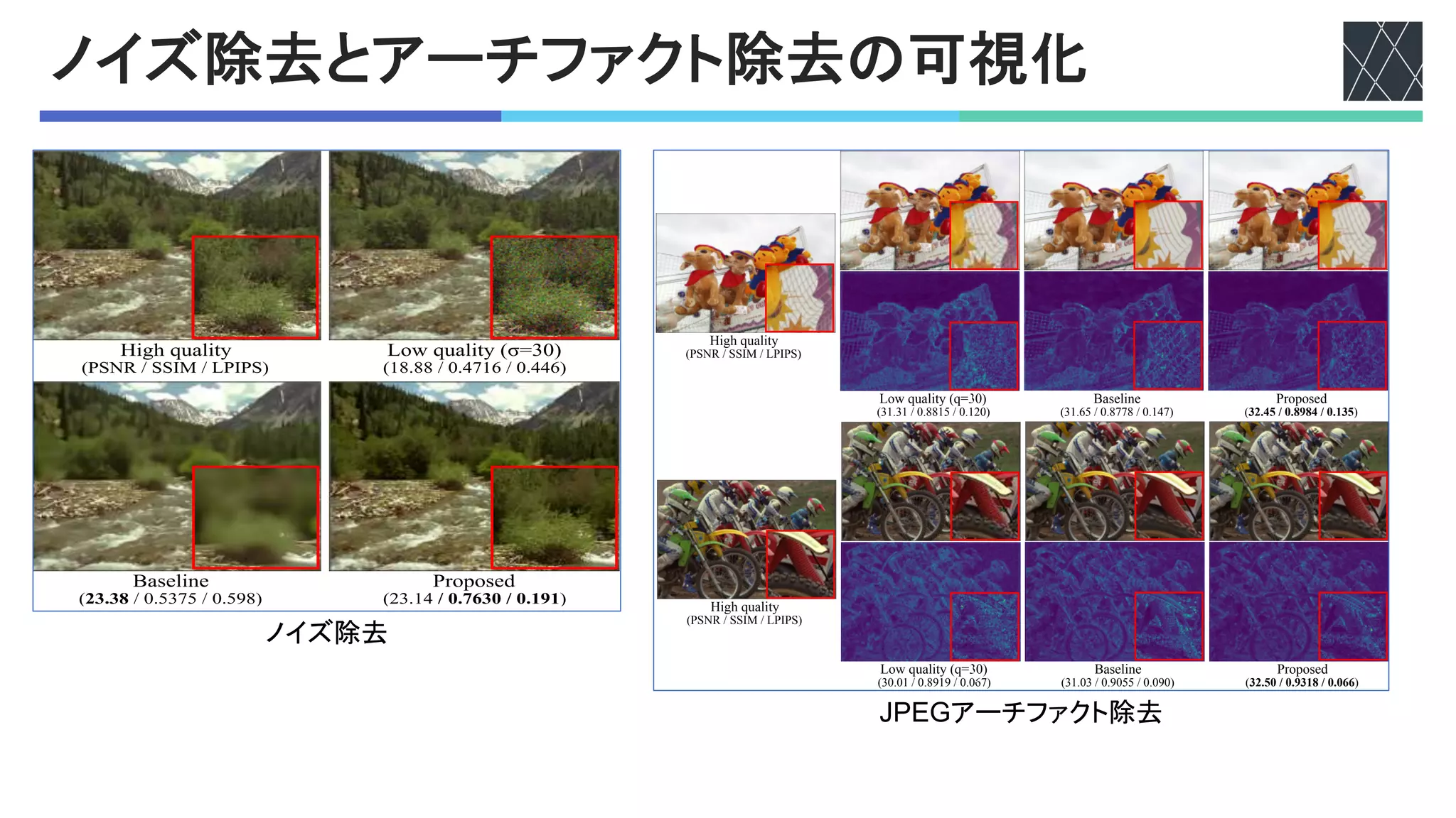
nノイズ除去
• ノイズの強さが違うもので比較
• aが大きいほど強いノイズ
n結果
• 過剰なスムージングを抑制
• 細かい構造を維持して
ノイズを除去
n!7FXアーチティファクト除去
• 圧縮の品質が違うもので比較
• bが低いほど強い圧縮
n結果
• 過剰な除去を抑制
• 全ての評価指標で性能向上
Table 4. Performance comparison on the color Gaussian denoising
task evaluated on the Kodak24 dataset. We train the model with
both mild (σ = 30) and severe noises (σ = 70) and test on the
mild setting. LPIPS [31] (lower is better) indicates the perceptual
distance between the network output and the ground-truth.
Model Train σ
Test (σ = 30)
PSNR ↑ SSIM ↑ LPIPS ↓
EDSR
30
31.92 0.8716 0.136
+ proposed +0.02 +0.0006 -0.004
EDSR
70
27.38 0.7295 0.375
+ proposed -2.51 +0.0696 -0.193
Table 5. Performance comparison on the color JPEG artifact re-
moval task evaluated on the LIVE1 [18] dataset. We train the
High quality
(PSNR / SSIM / LPIPS)
Low quality (σ=30)
(18.88 / 0.4716 / 0.446)
Table 4. Performance comparison on the color Gaussian denoising
task evaluated on the Kodak24 dataset. We train the model with
both mild (σ = 30) and severe noises (σ = 70) and test on the
mild setting. LPIPS [31] (lower is better) indicates the perceptual
distance between the network output and the ground-truth.
Model Train σ
Test (σ = 30)
PSNR ↑ SSIM ↑ LPIPS ↓
EDSR
30
31.92 0.8716 0.136
+ proposed +0.02 +0.0006 -0.004
EDSR
70
27.38 0.7295 0.375
+ proposed -2.51 +0.0696 -0.193
Table 5. Performance comparison on the color JPEG artifact re-
moval task evaluated on the LIVE1 [18] dataset. We train the
model with both mild (q = 30) and severe compression (q = 10)
and test on the mild setting.
Model Train q
Test (q = 30)
PSNR ↑ SSIM ↑ LPIPS ↓
EDSR
30
33.95 0.9227 0.118
+ proposed -0.01 -0.0002 +0.001
EDSR
10
32.45 0.8992 0.154
+ proposed +0.97 +0.0187 -0.023
4.4. Other low-level vision tasks
Fig
tas
σ
me
sm
JP
da
(lo

12. まとめ
n48に対する既存?0の分析
• 画像の構造的な変化が大きいものは使えない
n新たな手法5%ABC%D*'K)0を提案
• 48に効果がある
• K)0はモデルサイズが大きくデータセットが実世界から
収集されている場合に特に効果が大きい
• 8#"C48で4cd0を達成
• 他の低レベルの視覚タスクへの拡張性
• ノイズ除去
• !7FXアーティファクト除去

13. なぜ!"が必要なのか
n合成データセット
• システムの劣化関数により容易に学習サンプルを増強
• 合成データと実データの分布にはギャップ
• 実環境で性能を発揮できないことがある
• 解決には実データを使うことが必要
nデータ拡張
• 実データに対して使用
• 実データの収集にかかる時間とコストを減らせる

14. 従来の#$用の!"
n48に使われている?0手法
• 簡単な幾何学的操作
• 回転
• 並進
n8#V%ら E"DOGP9:;=Jによって有効性が確認 >0H*'0H0@

15. 特徴量空間の!"と%&',&'の調整
n特徴量空間の?0
• K"&GU)CV'KGL%M
• 4-"/#?D)M
n5%A)%A
• そのまま使う>9^eの領域@と
:`;VB性能を下げる
• 調整した設定
• 比率を:`;e
• 矩形領域でなくランダムピクセル

16. +-.'&*/0,10"&23/4'5'-,406+,"7
n表のような設定になっている
• 基本的にK)0の適用確率Mf;`:
• 合成データセットで485++*508+を学習する際のみMf:`9
• ノイズ除去，アーチファクト除去ではMf:`=
• 8#"C48では選択手法
に偏りを持たせる
• 5%ABC%DgZ:e
• その他g;:e

17. 想定する実環境での効果
n実世界での解像度にばらつきがある画像としてピンボケ写真でテスト
• _#]とGM-)&#;;でそれぞれ撮影された画像
• ベースラインは性能が低下するが
5%ABC%Dで学習したモデルは性能が低下しない
Table 3. Quantitative comparison (PSNR / SSIM) on SR (scale ×4) task in both synthetic and realistic settings. δ denotes the performance
gap between with and without augmentation. For synthetic case, we perform the ×2 scale pre-training.
Model # Params.
Synthetic (DIV2K dataset) Realistic (RealSR dataset)
Set14 (δ) Urban100 (δ) Manga109 (δ) RealSR (δ)
CARN
1.14M
28.48 (+0.00) / 0.7787 25.85 (+0.00) / 0.7779 30.17 (+0.00) / 0.9034 28.78 (+0.00) / 0.8134
+ proposed 28.48 (+0.00) / 0.7788 25.85 (+0.00) / 0.7780 30.16 (-0.01) / 0.9032 29.00 (+0.22) / 0.8204
RCAN
15.6M
28.86 (+0.00) / 0.7879 26.76 (+0.00) / 0.8062 31.24 (+0.00) / 0.9169 29.22 (+0.00) / 0.8254
+ proposed 28.92 (+0.06) / 0.7895 26.93 (+0.17) /0.8106 31.46 (+0.22) / 0.9190 29.49 (+0.27) / 0.8307
EDSR
43.2M
28.81 (+0.00) / 0.7871 26.66 (+0.00) / 0.8038 31.06 (+0.00) / 0.9151 28.89 (+0.00) / 0.8204
+ proposed 28.88 (+0.07) / 0.7886 26.80 (+0.14) / 0.8072 31.25 (+0.19) / 0.9163 29.16 (+0.27) / 0.8258
EDSR w/o CutBlur (Δ)
HR LR (input)
EDSR w/ CutBlur (Δ)
EDSR w/o CutBlur (Δ)
HR LR (input)
EDSR w/ CutBlur (Δ)
Figure 6. Qualitative comparison of the baseline and CutBlur model outputs. The inputs are the real-world out-of-focus photography (×2

18. ノイズ除去とアーチファクト除去の可視化
Proposed
(23.14 / 0.7630 / 0.191)
Baseline
(23.38 / 0.5375 / 0.598)
High quality
(PSNR / SSIM / LPIPS)
Low quality (σ=30)
(18.88 / 0.4716 / 0.446)
Figure 7. Comparison of the generalization ability in the denoising
task. Both the baseline and the proposed method are trained using
σ = 70 (severe) and tested with σ = 30 (mild). Our proposed
method effectively recovers the details while the baseline over-
smooths the input resulting in a blurry image.
JPEG artifact removal (color). We generate a synthetic
High quality
(PSNR / SSIM / LPIPS)
Proposed
(32.45 / 0.8984 / 0.135)
Baseline
(31.65 / 0.8778 / 0.147)
Low quality (q=30)
(31.31 / 0.8815 / 0.120)
High quality
High quality
(PSNR / SSIM / LPIPS)
Proposed
(32.45 / 0.8984 / 0.135)
Baseline
(31.65 / 0.8778 / 0.147)
Low quality (q=30)
(31.31 / 0.8815 / 0.120)
High quality
(PSNR / SSIM / LPIPS)
Proposed
(32.50 / 0.9318 / 0.066)
Baseline
(31.03 / 0.9055 / 0.090)
Low quality (q=30)
(30.01 / 0.8919 / 0.067)
ノイズ除去
6781アーチファクト除去