This document describes a new spatial-temporal attention graph convolution network (STAGCN) for traffic forecasting. STAGCN contains three key components: 1) a graph learning layer that learns both a static graph capturing global spatial relationships and a dynamic graph capturing local spatial changes, 2) an adaptive graph convolution layer, and 3) a gated temporal attention module using causal-trend attention to model long-term temporal dependencies by focusing on important historical information. Experimental results on four traffic datasets show STAGCN achieves better prediction accuracy than existing methods.
![Citation: Gu, Y.; Deng, L. STAGCN:
Spatial–Temporal Attention Graph
Convolution Network for Traffic
Forecasting. Mathematics 2022, 10,
1599. https://doi.org/10.3390/
math10091599
Academic Editors: Andrea Prati, Luis
Javier García Villalba and Vincent A.
Cicirello
Received: 9 April 2022
Accepted: 5 May 2022
Published: 8 May 2022
Publisher’s Note: MDPI stays neutral
with regard to jurisdictional claims in
published maps and institutional affil-
iations.
Copyright: © 2022 by the authors.
Licensee MDPI, Basel, Switzerland.
This article is an open access article
distributed under the terms and
conditions of the Creative Commons
Attribution (CC BY) license (https://
creativecommons.org/licenses/by/
4.0/).
mathematics
Article
STAGCN: Spatial–Temporal Attention Graph Convolution
Network for Traffic Forecasting
Yafeng Gu and Li Deng *
School of Science, Zhejiang Sci-Tech University, Hangzhou 310018, China; 202020102037@mails.zstu.edu.cn
* Correspondence: lideng75@zstu.edu.cn
Abstract: Traffic forecasting plays an important role in intelligent transportation systems. However,
the prediction task is highly challenging due to the mixture of global and local spatiotemporal depen-
dencies involved in traffic data. Existing graph neural networks (GNNs) typically capture spatial
dependencies with the predefined or learnable static graph structure, ignoring the hidden dynamic
patterns in traffic networks. Meanwhile, most recurrent neural networks (RNNs) or convolutional
neural networks (CNNs) cannot effectively capture temporal correlations, especially for long-term
temporal dependencies. In this paper, we propose a spatial–temporal attention graph convolution
network (STAGCN), which acquires a static graph and a dynamic graph from data without any prior
knowledge. The static graph aims to model global space adaptability, and the dynamic graph is
designed to capture local dynamics in the traffic network. A gated temporal attention module is
further introduced for long-term temporal dependencies, where a causal-trend attention mechanism
is proposed to increase the awareness of causality and local trends in time series. Extensive experi-
ments on four real-world traffic flow datasets demonstrate that STAGCN achieves an outstanding
prediction accuracy improvement over existing solutions.
Keywords: deep learning; traffic forecasting; graph convolution networks; attention mechanism;
spatial–temporal graph data
MSC: 68T07
1. Introduction
Traffic forecasting aims to predict future traffic conditions (e.g., traffic flow, interval
speed) based on historical traffic information that is as long as the prediction interval.
In general, traffic prediction tasks can be divided into two categories according to the
length of the prediction interval, namely short-term (5~30 min) and long-term (30~60 min)
prediction tasks [1]. Traffic forecasting also plays an important role in Intelligent Trans-
portation Systems (ITS), and it remains challenging due to its complex and changing
spatial–temporal dependencies in real-world road networks [2]. Traditional forecasting
methods, such as the autoregressive integrated moving average (ARIMA) model [3] and
Kalman filter [4], have a solid theoretical foundation, but they must rely on the stationarity
assumption. Furthermore, these methods are mainly applied to univariate time series,
which restricts their applications in real-world scenarios. With the development of data
availability and information computation, deep learning-based prediction work achieves
remarkable performance. Deep neural networks for spatiotemporal sequence modeling
are mainly divided into three categories: recurrent neural networks (RNNs), convolutional
neural networks (CNNs), and graph convolutional networks (GCNs) [5]. RNN-based
approaches employ hidden recurrent units to retain historical information, but they may
suffer from vanishing gradient issues when modeling long-term temporal dependencies
(i.e., temporal correlations between distant time steps in long sequences). CNN-based
approaches propagate spatiotemporal information under the assumption that traffic data
Mathematics 2022, 10, 1599. https://doi.org/10.3390/math10091599 https://www.mdpi.com/journal/mathematics](https://image.slidesharecdn.com/mathematics-10-01599-v2-220809053826-c54bffe1/75/mathematics-10-01599-v2-pdf-1-2048.jpg)
![Mathematics 2022, 10, 1599 2 of 16
are generated from grid-distributed sensors, and they fail to explicitly capture spatial corre-
lations in non-Euclidean data. GCN-based approaches receive widespread attention due to
their high adaptability in dealing with non-Euclidean data. At present, most GCNs rely on
the predefined static graph structure with prior knowledge. A fine-grained graph structure
will bring great improvements for prediction performance, and how to obtain the optimal
graph structure becomes a primary challenge. In most cases, complex spatiotemporal data
are not equipped with an explicit graph structure, because connections among arbitrary
nodes (e.g., sensors of traffic network) should be generated in a data-oriented manner.
Graph WaveNet [6] proposes a self-adaptive adjacency matrix to preserve hidden spatial
correlations. Wu et al. [7] extract a sparse graph adjacency matrix adaptively based on data
and updates the matrix during training. Yu et al. [8] introduce iterative learning for graph
learning by leveraging graph regularization. While the mentioned graph-based methods
have been successfully used in real-world applications, including but not limited to action
recognition, point cloud segmentation, and time series forecasting, they will still face the
following challenges:
• Global adaptability and local dynamics. Most GCNs only focus on constructing an
adaptive graph matrix to capture long-term or global space dependencies in traffic
data, while overlooking the fact that the correlation between local nodes is changing
significantly over time. As shown in Figure 1, sudden traffic accidents may lead to
local changes in spatial correlation among nodes. The primary question is how to keep
the balance between global adaptability and local dynamics in an end-to-end work.
• Long-term temporal correlations. Current graph-based methods are ineffective to
model long-term temporal dependencies. Existing methods either integrate GCNs into
RNNs or CNNs, in which small prediction errors at each time step may be magnified as
the prediction interval grows. This type of error forward propagation makes long-term
forecasting more challenging.
(a) Detection sensors on road network (b) Traffic flow of different detectors
Figure 1. Example of spatiotemporal dependencies in PEMSD8 Dataset. (a) Global space correlation
is dominated by the road network structure. (b) Sudden events, as marked with black boxes in
the figure.
In this paper, we propose a novel approach to overcome the aforementioned chal-
lenges. Our framework consists of three components: graph learning layer, adaptive graph
convolution layer, and gated temporal attention module. For challenge 1, we propose
a graph learning layer in which two types of graph matrices can be learned from data,
namely a static graph and dynamic graph. The static graph aims to explore global space
adaptability in traffic graph networks, and graph regularization is further employed to
control the quality of the static graph. The dynamic graph is designed to capture the
locally changing information among nodes. For challenge 2, we propose a gated temporal
attention module, which adopts multi-head self-attention to address long-term prediction
issues. In contrast to RNNs and CNNs, the attention mechanism aggregates temporal
features through a summation function with dynamically generated weights. This leads to
an effective global receptive field and allows the model to focus on significant historical](https://image.slidesharecdn.com/mathematics-10-01599-v2-220809053826-c54bffe1/75/mathematics-10-01599-v2-pdf-2-2048.jpg)
![Mathematics 2022, 10, 1599 3 of 16
information, which can alleviate error forward propagation. To be more aware of causality
and local trends in time series, we introduce a causal-trend attention mechanism instead of
using traditional multi-head attention directly. In summary, our main contributions are
as follows:
• We propose a novel graph learning layer to explore the interactions between global
space adaptability and local dynamics in traffic networks without any guidance of
prior knowledge. The static graph aims to model global adaptability, and the dynamic
graph is designed to capture local spatial changes.
• We propose a gated temporal attention module to model long-term temporal depen-
dencies. Furthermore, we design a causal-trend attention mechanism that enables our
model to extract causality and local trends in time series.
• Extensive experiments are conducted on four public traffic datasets, and the experi-
mental results show that our method consistently outperforms all baseline methods.
2. Related work
2.1. Traffic Forecasting
Traffic forecasting has been extensively studied in the past few decades. Earlier work
is usually based on the traditional statistical methods, such as ARIMA and the Kalman
filter. Although statistical methods are widely adopted for traffic forecasting due to their
simplicity and interpretability, they have to rely on the stationary assumption and do not
scale well for complex traffic data. Deep learning approaches can effectively capture the
non-linearity of traffic data. Many of them initially employed RNNs [9] or TCNs [10]
to model temporal dependency, ignoring the spatial correlations in traffic data. Later,
researchers used CNNs [11] to extract spatial dependencies in Euclidean space, but this
fails to effectively process non-Euclidean data and limits the prediction performance.
Recently, many studies have attempted to employ graph convolution methods to
model spatial and temporal dependencies in non-Euclidean road networks. Most of them
assume that a well-defined graph structure has already existed. Li et al. [12] integrate
diffusion convolution into gated recurrent units (GRUs), where the predefined graph ma-
trix is generated from road network distances. Now, many researchers are devoted to
finding optimal graph structures in a data-driven way. Wang et al. [13] propose a new adap-
tive feature graph to learn correlations between topological structures and node features.
Song et al. [14] propose a spatiotemporal graph to simultaneously capture the localized
spatiotemporal dependencies, which requires prior graph knowledge and additional graph
construction operation. The above graph-based methods mainly concentrate on adaptive
graph construction or heavily rely on the predefined graph structure, ignoring dynamic
correlations in traffic data.
2.2. Graph Convolutional Network
Graph convolutional networks (GCNs) have achieved extraordinary performance on
several types of graph-based tasks, such as node classification [15], link prediction [16],
and clustering [17]. From the perspective of convolution operators, GCNs have two
mainstreams, namely spectral approaches and spatial approaches. Spectral approaches
smooth graph signals in the spectral domain through Fourier transform. Spatial approaches
define convolution operations directly on the graph based on the topology structure.
Velickovic et al. [18] assign different weights to neighbor nodes via an attention mechanism.
Li et al. [19] incorporate residual connections to increase the depth of GCNs and alleviates
oversmoothing and vanishing gradient issues. In these methods, the graph adjacency matrix
is regarded as prior knowledge and is static throughout the training phase. Wang et al. [20]
employ distance metrics to adaptively learn a similarity graph weight matrix for label
learning. The generated matrix relies on dynamic node representation and may hamper
model performance on graphs where the node set keeps changing.](https://image.slidesharecdn.com/mathematics-10-01599-v2-220809053826-c54bffe1/75/mathematics-10-01599-v2-pdf-3-2048.jpg)
![Mathematics 2022, 10, 1599 4 of 16
2.3. Attention Mechanism
The attention mechanism has been widely used in diverse application domains due to
its high efficiency and flexibility in modeling dependencies. The core idea of the attention
mechanism is to adaptively focus on significant parts when processing massive amounts
of information. Fukui et al. [21] extend the attention mechanism to a response-based
visual explanation model and achieves remarkable performance. Yan et al. [22] employ
attention mechanisms to adaptively encode local and global point cloud context information.
Zheng et al. [23] propose a spatiotemporal attention mechanism to explore dynamic spatial
and non-linear temporal correlations. In this paper, we adopt an attention mechanism for
long-term temporal dependency modeling.
3. Methodology
3.1. Preliminaries
Traffic Networks: The traffic prediction task can be expressed as a typical spatiotempo-
ral series forecasting problem. We define the topological road network as a directed graph
G(V, A). Here, V is the set of N = |V| vertices representing detectors installed on the road.
The graph structure can be represented as a weighted adjacency matrix A ∈ RN×N, where
Ai,j 0 indicates the correlation between vertices vi and vj. In general, the values on the
diagonal of the initialized adjacency matrix A are equal to 1, which could avoid ignoring
the feature of the node itself. The traffic signals observed at time step t on traffic network G
can be defined as xt ∈ RN×C, where C denotes the feature dimension of vertices (e.g., traffic
flow, traffic speed).
Problem Statement: Given the historical observed P time steps traffic signals, denoted
as X = {xt1 , xt2 , . . . , xtp } ∈ RP×N×C, our goal is to predict next H time step traffic signals
Y = {xtp+1 , xtp+2 , . . . , xtp+h } ∈ RH×N×C.
Scaled Dot-Product Attention: The attention function aims to map a query and a set
of key–value pairs to an output, where the query and key–value pairs are all vectors. The
output is a weighted sum of values, where the weight assigned to each value is determined
jointly by a query and the corresponding key. The dot-product attention is a widely adopted
attention function, which enjoys remarkable properties such as time and space efficiency.
Finally, the output is as follows:
Attention(Q, K, V) = So f tMax(
Q · KT
√
dk
)V. (1)
where Q, K, V, and dk represent the query, keys, values, and dimensions, respectively.
3.2. Framework of STAGCN
Figure 2 illustrates the architecture of our proposed STAGCN model, which consists
of a static–dynamic graph learning layer, gated temporal attention module (Gated TAM),
and adaptive graph convolution layer (GCN). To explore the complex correlations between
global and local spatiotemporal dependencies, two types of graphs are learned from data,
i.e., static graph and dynamic graph. Gated TAM consists of two parallel temporal attention
layers, where causal-trend attention is proposed for long-term temporal dependencies. In
GCN, we employ two separate modules to aggregate spatial information based on the static
and dynamic graph. Every layer adopts residual connections and is skipped to the output
module. In more detail, the core components of our model are illustrated in the following.
3.3. Spatial Static–Dynamic Graph Learning Layer
3.3.1. Static Graph Learning
The spatial static graph learning layer aims to learn a static adaptive adjacency matrix,
which can capture the global spatial correlations among traffic data without the predefined](https://image.slidesharecdn.com/mathematics-10-01599-v2-220809053826-c54bffe1/75/mathematics-10-01599-v2-pdf-4-2048.jpg)
![Mathematics 2022, 10, 1599 5 of 16
graph structure. We employ node embedding to construct the static adjacency matrix [7,24],
denoted as follows:
M1 = tanh(E1 · θ1), (2)
M2 = tanh(E2 · θ2), (3)
As = So f tMax(ReLU(M1 · MT
2 )), (4)
where E1, E2 represent randomly initialized node embedding, whose parameters can be
learned during training, and θ1, θ2 are model parameters. We employ ReLU activation to
eliminate weak connections between nodes. So f tMax activation is adopted to normalize
the learned adjacency matrix.
Figure 2. The framework of STAGCN. The model consists of a spatial static–dynamic graph learning
layer, gated temporal attention module (Gated TAM), and adaptive graph convolution layer (GCN).
The input and learned spatiotemporal embedding are first passed through Gated TAM, followed
by the graph learning layer to obtain static and dynamic graphs. Then, feature representation and
graphs are passed to GCN for spatial modeling.
A well-defined graph structure can bring significant benefits to the prediction task,
so it is essential to control the sparsity and smoothness of the learned graph structure.
Therefore, we add a graph regularization loss function following previous work [8] to
improve the quality of the graph structure. For the learned global adjacency matrix A and
the given node feature matrix XF = (x1, x2, . . . , xN) ∈ RN×D, the graph regularization loss
is as follows:
LG = α
1
N2
N
∑
i,j
Ai,jkxi − xjk2
+ βkAk2
F, (5)
where α, β are model hyperparameters and k·k2
F denotes the Frobenius norm of the matrix.
A widely recognized assumption is that graph signals change smoothly through adjacent
nodes, so minimizing the first term will force adjacent nodes to have similar features.
However, only restricting the smoothness of the graph will lead to A = 0, so we add the
Frobenius norm of the matrix to control the sparsity of the graph. Instead of applying
regularization to all inputs or node embedding at once, we apply it to the node output
features in the gradient update section.
3.3.2. Dynamic Graph Learning
For spatiotemporal traffic data, the dependencies among nodes are very likely to
dynamically change over time, e.g., traffic congestion upstream will affect the traffic flow
downstream. Therefore, only applying the static graph structure may fail to grasp such](https://image.slidesharecdn.com/mathematics-10-01599-v2-220809053826-c54bffe1/75/mathematics-10-01599-v2-pdf-5-2048.jpg)
![Mathematics 2022, 10, 1599 6 of 16
local dynamic correlation. To this end, we introduce a dynamic graph that can adaptively
alter the relationship among nodes at all time steps.
The key idea of our method is to adopt a self-attention mechanism to calculate the
spatial correlations among nodes. To be concrete, given the dynamic node feature set
Xt ∈ RN×dmodel , the dynamic spatial adjacency matrix can be denoted as:
Ad = So f tMax(
Xt · XT
t
√
dmodel
) ∈ RN×N
. (6)
3.4. Adaptive Graph Convolution Module
A graph convolution network is widely adopted to process non-grid or unstructured
data and aims to extract a high-level node feature representation through the neighborhood
aggregation method. Li et al. [12] proposed a graph diffusion convolution layer to learn
node representations by iteratively aggregating adjacent node features. For a k-layer
diffusion model, the l-th layer information propagation step can be formulated as:
H(l)
= ÂH(l−1)
W(l)
, (7)
where H(l) ∈ RN×dl denotes the output of node features of layer l, H(0) represents the
initialized node feature, Â denotes the normalized adjacency matrix, and W(l) ∈ Rdl−1×dl
denotes the layer-specific model weight matrix.
However, a common challenge faced by graph convolution operation is that the node
hidden states will become more similar when graph convolution layers go deeper. On
the other hand, a shallow graph convolution network cannot sufficiently propagate the
edge node information to the entire graph. Depending on the application, an appropriate
receptive field or neighborhood size should be more desirable. To achieve this, motivated
by [25], we explore an adaptive attention mechanism that can adaptively adjust the neigh-
borhood size of each node. As shown in Figure 3, compared to simply concatenating
[H(0), H(1), . . . , H(k)] to combine different layers, the mechanism can maintain a better bal-
ance between local and global information propagation, which leads to more discriminative
node features. The mechanism formula is as follows:
H(0)
= MLP(X), ∈RN×D
H(l)
= αH(0)
+ (1 − α)ÂH(l−1)
, ∈RN×D
P = stack(H(0)
, H(1)
. . . , H(k)
), ∈RN×(k+1)×D
S = reshape(σ(PW)), ∈RN×1×(k+1)
Z = squeeze(SP), ∈RN×D
(8)
where H(0) denotes the feature matrix derived from applying MLP to the initialized node
features X, W represents the trainable model parameters, and S represents the attention
score for each layer. σ denotes the activation function and we employ sigmoid here. α
is a hyperparameter that controls the original node feature retention rate to preserve the
local property.
To explore the interaction between global spatial adaptability and local dynamics,
we apply static and dynamic graph structures to the adaptive graph convolution layer
separately, i.e., replacing  with learned As and Ad. The final output is as follows:
Z = Zstatic + Zdynamic. (9)
3.5. Gated Temporal Attention Module
The temporal attention module applies attention mechanisms to extract long-term
temporal dependencies. As shown in Figure 2, this module consists of two parallel temporal
attention layers, where the causal-trend attention mechanism is proposed. One layer is](https://image.slidesharecdn.com/mathematics-10-01599-v2-220809053826-c54bffe1/75/mathematics-10-01599-v2-pdf-6-2048.jpg)
![Mathematics 2022, 10, 1599 7 of 16
followed by a tangent hyperbolic activation function, which works as a filter. The other
layer is followed by a sigmoid activation function as a gate, which controls the information
that needs to be passed to the next module.
(a) (b)
Figure 3. An illustration of the proposed adaptive graph convolution module. This module can
adaptively adjust the node neighborhood size according to the application. (a) K-hop neighbor nodes,
(b) adaptive neighborhood size adjustment.
Multi-head self-attention [26] can effectively attend to information from different
representation subspaces. The basic operation in multi-head self-attention has been defined
in Equation (1), where all the keys, values, and queries are the same sequence representation,
i.e., Q = K = V. It first linearly projects the queries, keys, and values to different feature
subspaces and then the attention function is performed in parallel. Lastly, the outputs are
concatenated and once projected again. Formally, the final value can be defined as:
MultiHead(Q, K, V) = ⊕(head1, . . . , headh)Wo
headj = Attention(QWj
Q
, KWj
K
, VWj
V
),
(10)
where Wj
Q
, Wj
K
, Wj
V
are the projection matrices applied to Q, K, V, Wo is the output
projection matrix, and the subscript h represents the number of attention heads. The multi-
head self-attention can selectively focus on important information and efficiently explore
the correlation between arbitrary elements in the sequence, thus leading to a flexible global
receptive field.
Note that the attention mechanism was originally proposed to process discrete word
sequences and it fails to learn the causality and local trends inherent in time series. The
traditional attention mechanism may incorrectly match two points in the sequence because
they are numerically similar. However, two points will exhibit significantly different local
trends (e.g., uptrend or downtrend). Inspired by ASTGNN [27], we introduce a causal-trend
attention mechanism to explore traffic series’ temporal property, as shown in Figure 4. To
take local contextual information into consideration, we replace the projection operation on
the queries and keys with 1D convolution. For masking future information, we employ
causal convolution [28] on the values. Contextual information is taken as input and future
information will not be intercepted, thus eventually benefiting the entire model to be aware
of local changes and effectively fit predicted values. Formally, our causal-trend attention
mechanism is defined as follows:
CTAttention(Q, K, V) = ⊕(head1, . . . , headh)Wo
headj = Attention(Q · ΦQ
j , K · ΦK
j , V · ΨV
j ),
(11)
where ΦQ
j , ΦK
j are 1D convolution kernel parameters and ΨV
j represents causal convolution
kernel parameter.](https://image.slidesharecdn.com/mathematics-10-01599-v2-220809053826-c54bffe1/75/mathematics-10-01599-v2-pdf-7-2048.jpg)
![Mathematics 2022, 10, 1599 8 of 16
Figure 4. Comparison of traditional self-attention mechanism and our causal-trend attention mech-
anism. Traditional self-attention mechanisms may incorrectly match points in the sequence with
similar values shown in (a). Our causal-trend attention mechanism is shown in (c), which replaces the
projection operations with 1D and causal convolution. As shown in (b), such awareness of locality
and causality in time series can correctly match the most relevant feature in the series.
3.6. Extra Components
In this section, we introduce extra components that the SATGCN adopts to enhance
its representation power.
3.6.1. Spatial–Temporal Embedding
Though our method can capture spatial and temporal dynamic properties through
separate modules, we ignore the spatioemporal heterogeneity and intrinsic signal order.
Inspired by STSGCN [14], we equip position embedding into the model so that we can
take into account both spatial and temporal information, which can enhance the ability
to model spatial–temporal correlations. For the traffic signal sequence XG ∈ RN×T×C,
we create a learnable temporal embedding matrix TE ∈ RT×C and spatial embedding
matrix SE ∈ RN×C. After the training phase, the embedding matrix will contain extra
spatial–temporal information to improve the prediction performance.
We add the embedding matrix to the input traffic signal sequence with broadcasting
operation for augmenting sequence representation:
XG+Temb+Semb = XG + TE + SE, (12)
3.6.2. Loss Function
Compared with most current approaches, we learn the graph structure and optimize
model parameters by minimizing a hybrid loss function that combines graph regularization
loss and prediction loss. The hybrid loss function is as follows:
L(Y, b
Y) = LG + L1loss(Y, b
Y). (13)
where Y, b
Y denote the ground truth and predictions of the model, L1loss is computed for
back-propagation, and graph regularization loss LG is formulated following Equation (5).
4. Experiments
4.1. Datasets
We verify the performance of STAGCN on four public traffic network datasets,
PEMS03, PEMS04, PEMS07, and PEMS08, collected from the Caltrans Performance Mea-
surement System (PEMS).
PEMSD3: The dataset records the highway traffic flow information in the North
Central Area. There are 358 road detectors placed in different regions, and the data were
collected from 1 September 2018 to 30 November 2018.
PEMSD4: The dataset contains traffic flow data in the San Francisco Bay Area. We
select 307 road detectors and capture the data from 1 January 2018 to 28 February 2018.
PEMSD7: The dataset refers to the traffic information collected from 883 loop detectors
on Los Angeles County highways from 1 May 2017 to 31 August 2018.](https://image.slidesharecdn.com/mathematics-10-01599-v2-220809053826-c54bffe1/75/mathematics-10-01599-v2-pdf-8-2048.jpg)
![Mathematics 2022, 10, 1599 9 of 16
PEMSD8: The dataset includes the traffic flow information in the San Bernardino area.
It is gathered from 170 road detectors within the period from 1 July 2016 to 31 August 2016.
These datasets record traffic flow statistics on the highways of California and are
aggregated into 5-min windows, which means that the sequence has 12 time steps in one
hour. We utilize the historical data for the 12 time steps (1 h) to predict traffic flow for the
next hour. In addition, we employ the same data pre-processing measures as STSGCN,
and the data are normalized via the Z-score method. Further detailed dataset statistical
information is provided in Table 1.
Table 1. Dataset statistics.
Datasets Samples Nodes Time Range
PEMS03 26,208 358 1 September 2018–30 November 2018
PEMS04 16,992 307 1 January 2018–28 February 2018
PEMS07 28,224 883 1 May 2017–31 August 2017
PEMS08 17,856 170 1 July 2016–31 August 2016
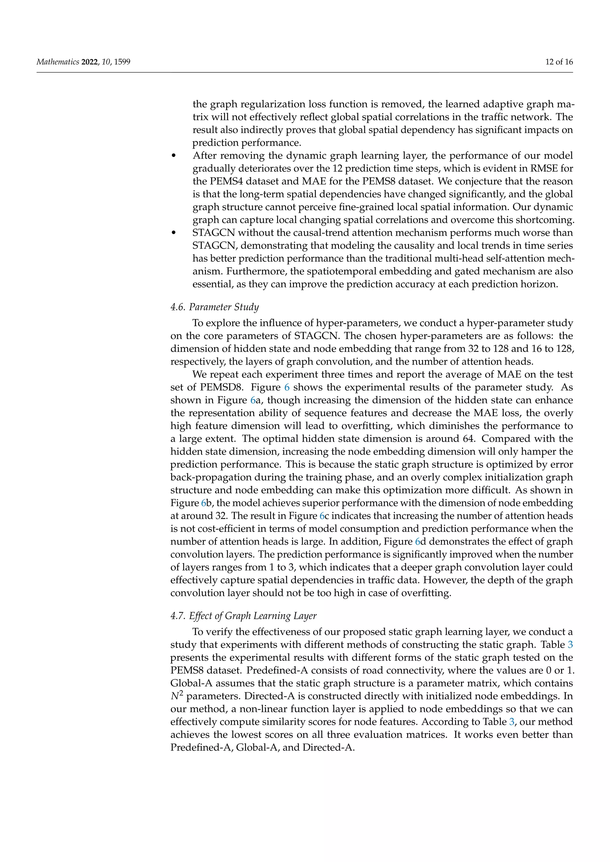
4.2. Experimental Setting
We split all datasets with ratio 6:2:2 into training sets, validation sets, and testing
sets [29]. We use Equation (8) for the graph convolution operation and diffusion step k = 3.
The size of the hidden state is set to 64, and the dimension of node embeddings is set to
32. The number of attention heads is set to 8, and early stopping is employed to avoid
overfitting. In addition, we train our model using the Adam optimizer [30] with an initial
learning rate of 0.001. We choose mean absolute error (MAE), root mean squared error
(RMSE), and mean absolute percentage error (MAPE) to evaluate the performance of our
model. The evaluation metrics’ formulas are as follows:
(1) Mean absolute error (MAE):
MAE =
1
n
n
∑
t=1
|Yt − b
Yt|, (14)
MAE represents the average absolute difference between the predicted values and the
ground truth. The smaller the MAE value, the better the prediction performance.
(2) Root mean square error (RMSE):
RMSE =
s
1
n
n
∑
t=1
(Yt − b
Yt)2, (15)
RMSE describes how far predictions fall from measured true values using Euclidean
distance. It is mainly used to evaluate the prediction error.
(3) Mean absolute percentage error (MAPE):
MAPE =
1
n
n
∑
t=1
|
Yt − b
Yt
Yt
|. (16)
MAPE measures the prediction accuracy as a percentage and works best if the data
have no extreme values.
4.3. Baseline Methods
• SVR: Support vector regression [31], which uses a support vector machine for prediction tasks.
• FC-LSTM: LSTM encoder–decoder predictor model, which employs a recurrent neural
network with fully connected LSTM hidden units [32].
• DCRNN: Diffusion convolutional recurrent neural network [12], which integrates
diffusion graph convolution into gated recurrent units.](https://image.slidesharecdn.com/mathematics-10-01599-v2-220809053826-c54bffe1/75/mathematics-10-01599-v2-pdf-9-2048.jpg)
![Mathematics 2022, 10, 1599 10 of 16
• STGCN: Spatio–temporal graph convolutional network [33], which adopts graph convo-
lutional and causal convolutional layers to model spatial and temporal dependencies.
• ASTGCN (r): Attention-based spatial-temporal graph convolutional network [34],
which designs a spatiotemporal attention mechanism for traffic forecasting. It ensem-
bles three different components to model the periodicity of traffic data, and we only
use its recent input segment for a fair comparison.
• STSGCN: Spatial–temporal synchronous graph convolutional network [14], which
captures correlations directly through a localized spatial–temporal graph.
• AGCRN: Adaptive graph convolutional recurrent network [35], which captures the
node-specific spatial and temporal dynamics through a generated adaptive graph.
• STFGNN: Spatial–temporal fusion graph neural networks [36], which use the dynamic
time warping algorithm (DTW) for graph construction to explore local and global
spatial correlations.
4.4. Experimental Results
Table 2 quantitatively presents the performance of our network on the PEMS datasets
compared to other representative methods. STAGCN obtains superior performance with
overall accuracy. We can observe that (1) SVR and FC-LSTM only take temporal correla-
tions into consideration and ignore the spatial dependencies in road networks. Therefore,
their performance is the worst. Especially, as shown in Table 2, SVR and FC-LSTM drop
significantly on the PEMS04 and PEMS07 datasets with more detection nodes. GCN-based
networks consistently outperform SVR and LSTM, demonstrating that graph convolution
can effectively capture spatial heterogeneity in time series. For instance, urban and rural
traffic flows have similar trend fluctuations during rush hours, but urban traffic is signifi-
cantly higher than rural traffic. (2) Adaptive graph network AGCRN surpasses pre-defined
graph models including DCRNN, ASTGCN, and STGCN by a large margin, indicating
that data-driven spatial dependency modeling plays an integral role in traffic forecasting
tasks. In most cases, the predefined graph is not optimal and struggles to adapt to complex
spatiotemporal traffic data. Compared with the predefined graph structure, the learned
adaptive graph matrix can uncover unseen graph structures automatically from the data,
without any guidance of prior knowledge. (3) Compared to other graph-based works,
STAGCN achieves superior performance, especially on the RMSE metric, for all datasets.
We argue that our static–dynamic graph learning layer significantly improves the capability
to capture local changing spatial heterogeneity and global spatial dependencies. The spatial
dependencies between different locations are highly dynamic, which is determined by
real-time traffic conditions and road networks. All the above baseline methods fail to
model this dynamic attribute of the traffic network, restricting the prediction performance.
(4) DCRNN and AGCRN are the typical RNN-based traffic forecasting works. Limited
by the capability to model long-term temporal dependencies, their forecasting accuracy is
much lower than our method. CNN-based forecasting works such as STGCN employ 1D
convolution or TCN for temporal dependencies. Similar to the RNN-based works, it cannot
effectively capture long-term temporal dependencies due to the size of the convolution
kernel. Compared with RNN and CNN-based works, our temporal modeling layer based
on the causal-trend attention mechanism can mitigate prediction error propagation to some
extent, and further improve the prediction accuracy.
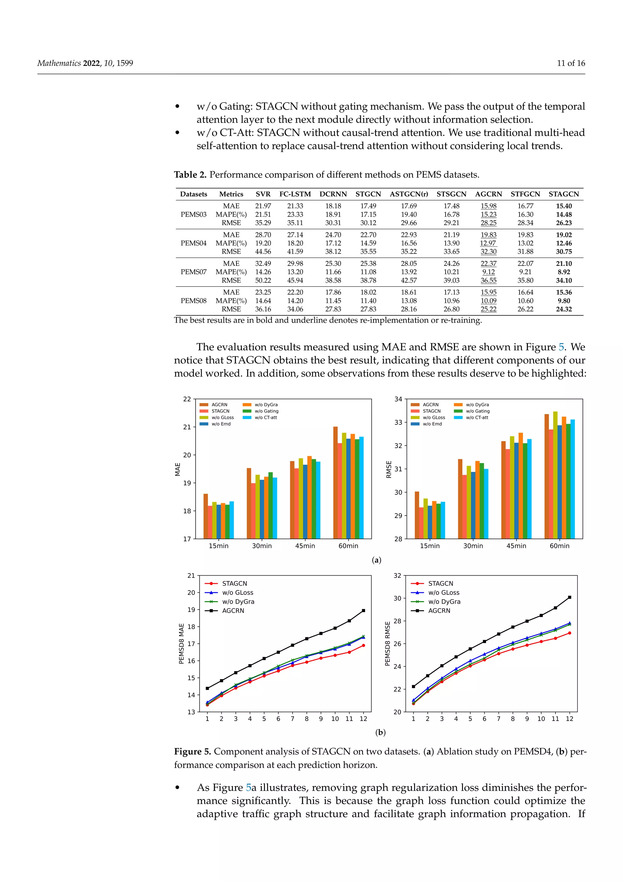
4.5. Ablation Study
To further investigate the effectiveness of different components that contribute to the
superior performance of our model, we conduct ablation studies on the PEMS4 and PEMS8
datasets. We name the models without different components as follows:
• w/o GLoss: STAGCN without graph regularization loss.
• w/o Emb: STAGCN without spatial and temporal embedding.
• w/o DyGra: STAGCN without dynamic graph learning layer. We only use a static
graph learning layer to adaptively model spatial correlation.](https://image.slidesharecdn.com/mathematics-10-01599-v2-220809053826-c54bffe1/75/mathematics-10-01599-v2-pdf-10-2048.jpg)
![Mathematics 2022, 10, 1599 15 of 16
methods. However, our model suffers from some inadequacies. For example, we argue that
there should be information interaction between the static and dynamic graphs, and the
two graph structures could complement each other. In the future, it would be worthwhile
to explore the interaction between the static and dynamic graph structures and how to
accelerate the inference speed of our proposed network. We will also attempt to apply our
model to other multivariate time series forecasting tasks.
Author Contributions: Y.G. conceived and designed the experiments, analyzed the data, and wrote
the paper. L.D. supervised the work, helped with designing the experimental framework, and edited
the manuscript. All authors have read and agreed to the published version of the manuscript.
Funding: This work was supported by grants from the National Natural Science Foundation of China
(61806204) and the Basic Public Welfare Research Project of Zhejiang Province (LGF22F020020).
Institutional Review Board Statement: Not applicable.
Informed Consent Statement: Not applicable.
Data Availability Statement: Not applicable.
Conflicts of Interest: The authors declare no conflict of interest.
References
1. Huang, R.; Huang, C.; Liu, Y.; Dai, G.; Kong, W. LSGCN: Long Short-Term Traffic Prediction with Graph Convolutional Networks.
In Proceedings of the Twenty-Ninth International Joint Conference on Artificial Intelligence, Yokohama, Japan, 11–17 July 2020;
pp. 2355–2361.
2. Fang, Y.; Qin, Y.; Luo, H.; Zhao, F.; Zeng, L.; Hui, B.; Wang, C. CDGNet: A Cross-Time Dynamic Graph-based Deep Learning
Model for Traffic Forecasting. arXiv 2021, arXiv:2112.02736.
3. Williams, B.M.; Hoel, L.A. Modeling and forecasting vehicular traffic flow as a seasonal ARIMA process: Theoretical basis and
empirical results. J. Transp. Eng. 2003, 129, 664–672. [CrossRef]
4. Guo, J.; Huang, W.; Williams, B.M. Adaptive Kalman filter approach for stochastic short-term traffic flow rate prediction and
uncertainty quantification. Transp. Res. Part C Emerg. Technol. 2014, 43, 50–64. [CrossRef]
5. Lim, B.; Zohren, S. Time-series forecasting with deep learning: A survey. Philos. Trans. R. Soc. A 2021, 379, 20200209. [CrossRef]
[PubMed]
6. Wu, Z.; Pan, S.; Long, G.; Jiang, J.; Zhang, C. Graph WaveNet for Deep Spatial-Temporal Graph Modeling. In Proceedings of the
IJCAI, Macao, China, 10–16 August 2019; pp. 1907–1913.
7. Wu, Z.; Pan, S.; Long, G.; Jiang, J.; Chang, X.; Zhang, C. Connecting the dots: Multivariate time series forecasting with graph
neural networks. In Proceedings of the 26th ACM SIGKDD International Conference on Knowledge Discovery Data Mining,
Virtual Event, 6–10 July 2020; pp. 753–763.
8. Chen, Y.; Wu, L.; Zaki, M. Iterative deep graph learning for graph neural networks: Better and robust node embeddings. Adv.
Neural Inf. Process. Syst. 2020, 33, 19314–19326.
9. Zhao, Z.; Chen, W.; Wu, X.; Chen, P.C.; Liu, J. LSTM network: A deep learning approach for short-term traffic forecast. IET Intell.
Transp. Syst. 2017, 11, 68–75. [CrossRef]
10. Liu, Y.; Dong, H.; Wang, X.; Han, S. Time series prediction based on temporal convolutional network. In Proceedings of the
2019 IEEE/ACIS 18th International Conference on Computer and Information Science (ICIS), Beijing, China, 17–19 June 2019;
pp. 300–305.
11. Yan, S.; Xiong, Y.; Lin, D. Spatial temporal graph convolutional networks for skeleton-based action recognition. In Proceedings of
the Thirty-Second AAAI Conference on Artificial Intelligence, New Orleans, LA, USA, 2–7 February 2018; pp. 3482–3489.
12. Li, Y.; Yu, R.; Shahabi, C.; Liu, Y. Diffusion Convolutional Recurrent Neural Network: Data-Driven Traffic Forecasting. In
Proceedings of the International Conference on Learning Representations, Vancouver, BC, Canada, 30 April–3 May 2018.
13. Wang, X.; Zhu, M.; Bo, D.; Cui, P.; Shi, C.; Pei, J. Am-gcn: Adaptive multi-channel graph convolutional networks. In Proceedings
of the 26th ACM SIGKDD International Conference on Knowledge Discovery Data Mining, Virtual Event, 6–10 July 2020;
pp. 1243–1253.
14. Song, C.; Lin, Y.; Guo, S.; Wan, H. Spatial-temporal synchronous graph convolutional networks: A new framework for spatial-
temporal network data forecasting. In Proceedings of the AAAI Conference on Artificial Intelligence, New York, NY, USA, 7–12
February 2020; Volume 34, pp. 914–921.
15. Kipf, T.N.; Welling, M. Semi-supervised classification with graph convolutional networks. In Proceedings of the International
Conference on Learning Representations, Toulon, France, 24–26 April 2017.
16. Zhang, M.; Chen, Y. Link prediction based on graph neural networks. In Proceedings of the Advances in Neural Information
Processing Systems, Montreal, QC, Canada, 3–8 December 2018; pp. 5165–5175.](https://image.slidesharecdn.com/mathematics-10-01599-v2-220809053826-c54bffe1/75/mathematics-10-01599-v2-pdf-15-2048.jpg)
![Mathematics 2022, 10, 1599 16 of 16
17. Zhang, C.; Song, D.; Huang, C.; Swami, A.; Chawla, N.V. Heterogeneous graph neural network. In Proceedings of the 25th ACM
SIGKDD International Conference on Knowledge Discovery Data Mining, Anchorage, AK, USA, 4–8 August 2019; pp. 793–803.
18. Velickovic, P.; Cucurull, G.; Casanova, A.; Romero, A.; Lio, P.; Bengio, Y. Graph attention networks. Stat 2018, 1050, 4.
19. Li, G.; Muller, M.; Thabet, A.; Ghanem, B. Deepgcns: Can gcns go as deep as cnns? In Proceedings of the IEEE/CVF International
Conference on Computer Vision, Seoul, Korea, 27–28 October 2019; pp. 9267–9276.
20. Wang, D.B.; Zhang, M.L.; Li, L. Adaptive graph guided disambiguation for partial label learning. IEEE Trans. Pattern Anal. Mach.
Intell. 2021 . [CrossRef] [PubMed]
21. Fukui, H.; Hirakawa, T.; Yamashita, T.; Fujiyoshi, H. Attention branch network: Learning of attention mechanism for visual
explanation. In Proceedings of the IEEE/CVF conference on Computer Vision and Pattern Recognition, Seoul, Korea, 27–28
October 2019; pp. 10705–10714.
22. Yan, X.; Zheng, C.; Li, Z.; Wang, S.; Cui, S. Pointasnl: Robust point clouds processing using nonlocal neural networks with
adaptive sampling. In Proceedings of the IEEE/CVF Conference on Computer Vision and Pattern Recognition, Seattle, WA, USA,
14–19 June 2020; pp. 5589–5598.
23. Zheng, C.; Fan, X.; Wang, C.; Qi, J. Gman: A graph multi-attention network for traffic prediction. In Proceedings of the AAAI
Conference on Artificial Intelligence, New York, NY, USA, 7–12 February 2020; Volume 34, pp. 1234–1241.
24. Li, Z.; Zhang, G.; Xu, L.; Yu, J. Dynamic Graph Learning-Neural Network for Multivariate Time Series Modeling. arXiv 2021,
arXiv:2112.03273.
25. Liu, M.; Gao, H.; Ji, S. Towards deeper graph neural networks. In Proceedings of the 26th ACM SIGKDD International Conference
on Knowledge Discovery Data Mining, Virtual Event, 6–10 July 2020; pp. 338–348.
26. Vaswani, A.; Shazeer, N.; Parmar, N.; Uszkoreit, J.; Jones, L.; Gomez, A.N.; Kaiser, Ł.; Polosukhin, I. Attention is all you need. In
Proceedings of the Advances in Neural Information Processing Systems, Long Beach, CA, USA, 4–9 December 2017; Volume 30.
27. Guo, S.; Lin, Y.; Wan, H.; Li, X.; Cong, G. Learning dynamics and heterogeneity of spatial-temporal graph data for traffic
forecasting. IEEE Trans. Knowl. Data Eng. 2021 . [CrossRef]
28. Oord, A.V.D.; Dieleman, S.; Zen, H.; Simonyan, K.; Vinyals, O.; Graves, A.; Kalchbrenner, N.; Senior, A.; Kavukcuoglu, K.
Wavenet: A generative model for raw audio. arXiv 2016, arXiv:1609.03499.
29. Demšar, J. Statistical comparisons of classifiers over multiple data sets. J. Mach. Learn. Res. 2006, 7, 1–30.
30. Kingma, D.P.; Ba, J. Adam: A Method for Stochastic Optimization. In Proceedings of the International Conference on Learning
Representations, San Diego, CA, USA, 7–9 May 2015.
31. Drucker, H.; Burges, C.J.; Kaufman, L.; Smola, A.; Vapnik, V. Support vector regression machines. Adv. Neural Inf. Process. Syst.
1996, 9, 155–161.
32. Sutskever, I.; Vinyals, O.; Le, Q.V. Sequence to sequence learning with neural networks. In Proceedings of the Advances in
Neural Information Processing Systems, Montreal, QC, Canada, 3–8 December 2014; Volume 27.
33. Yu, B.; Yin, H.; Zhu, Z. Spatio-Temporal Graph Convolutional Networks: A Deep Learning Framework for Traffic Forecasting. In
Proceedings of the IJCAI, Stockholm, Sweden, 13–19 July 2018; pp. 3634–3640.
34. Guo, S.; Lin, Y.; Feng, N.; Song, C.; Wan, H. Attention based spatial-temporal graph convolutional networks for traffic flow
forecasting. In Proceedings of the AAAI Conference on Artificial Intelligence, Honolulu, HI, USA, 27–28 January 2019; Volume 33,
pp. 922–929.
35. Bai, L.; Yao, L.; Li, C.; Wang, X.; Wang, C. Adaptive graph convolutional recurrent network for traffic forecasting. Adv. Neural Inf.
Process. Syst. 2020, 33, 17804–17815.
36. Li, M.; Zhu, Z. Spatial-temporal fusion graph neural networks for traffic flow forecasting. In Proceedings of the AAAI Conference
on Artificial Intelligence, Virtually, 2–9 February 2021; Volume 35, pp. 4189–4196.](https://image.slidesharecdn.com/mathematics-10-01599-v2-220809053826-c54bffe1/75/mathematics-10-01599-v2-pdf-16-2048.jpg)


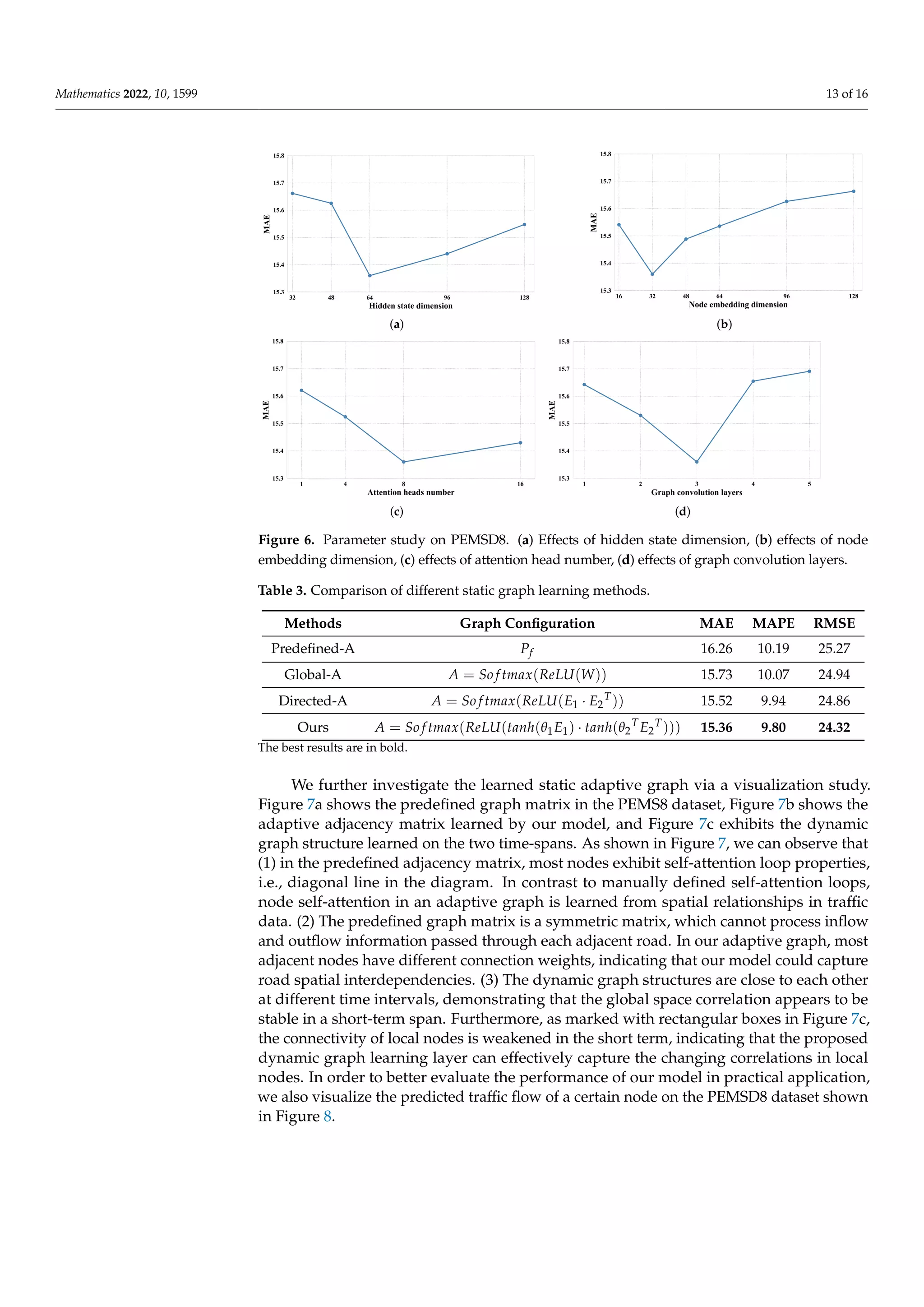
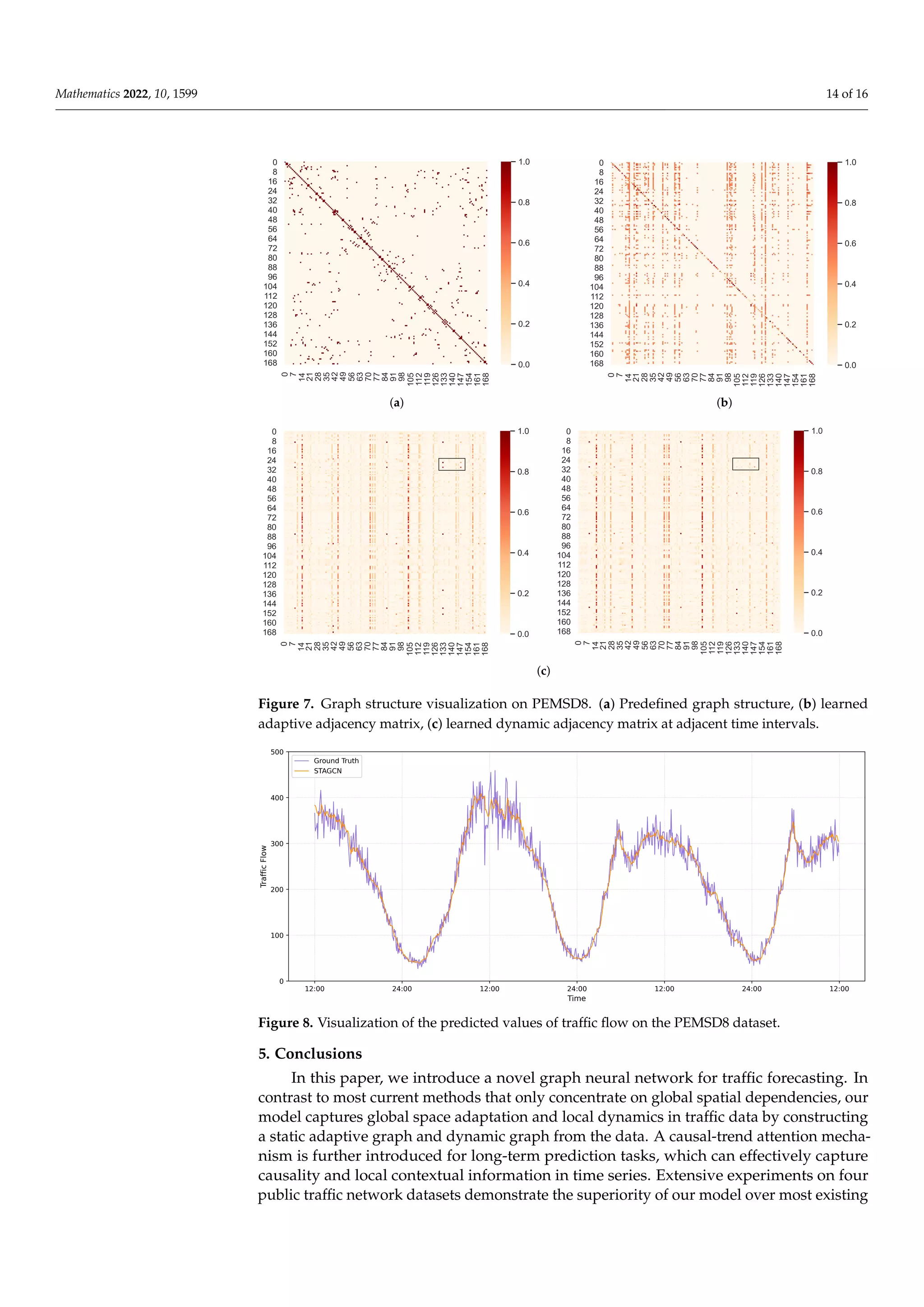
![[20240520_LabSeminar_Huy]DSTAGNN: Dynamic Spatial-Temporal Aware Graph Neural...](https://cdn.slidesharecdn.com/ss_thumbnails/20240520labseminarhuydstagnn-240520123156-67d80b3a-thumbnail.jpg?width=640&height=640&fit=bounds)
![[20240617_LabSeminar_Huy]Long-term Spatio-Temporal Forecasting via Dynamic Mu...](https://cdn.slidesharecdn.com/ss_thumbnails/20240617labseminarhuylstf-240624082154-84b13b22-thumbnail.jpg?width=640&height=640&fit=bounds)
![[20240325_LabSeminar_Huy]Spatial-Temporal Fusion Graph Neural Networks for Tr...](https://cdn.slidesharecdn.com/ss_thumbnails/20240325labseminarhuystfgnn-240409103218-8b4b7f23-thumbnail.jpg?width=640&height=640&fit=bounds)

![[20240805_LabSeminar_Huy]GPT-ST: Generative Pre-Training of Spatio-Temporal G...](https://cdn.slidesharecdn.com/ss_thumbnails/20240805labseminarhuygpt-st-240806102941-cd305d0d-thumbnail.jpg?width=640&height=640&fit=bounds)

![[20240703_LabSeminar_Huy]MakeGNNGreatAgain.pptx](https://cdn.slidesharecdn.com/ss_thumbnails/20240703labseminarhuymakegnngreatagain-240704111952-a7569149-thumbnail.jpg?width=640&height=640&fit=bounds)
![[20240318_LabSeminar_Huy]GSTNet: Global Spatial-Temporal Network for Traffic ...](https://cdn.slidesharecdn.com/ss_thumbnails/20240318labseminarhuygstnet-240409103756-4593be7d-thumbnail.jpg?width=640&height=640&fit=bounds)
![[20240408_LabSeminar_Huy]PivotalSTGNN.pptx](https://cdn.slidesharecdn.com/ss_thumbnails/20240408labseminarhuypivotalstgnn-240408123002-61e9cc31-thumbnail.jpg?width=640&height=640&fit=bounds)

![[20240710_LabSeminar_Huy]PDFormer: Propagation Delay-Aware Dynamic Long-Range...](https://cdn.slidesharecdn.com/ss_thumbnails/20240710labseminarhuypdformer-240723105641-9851ce9f-thumbnail.jpg?width=640&height=640&fit=bounds)
![[20240624_LabSeminar_Huy]Towards Dynamic Spatial-Temporal Graph Learning: A D...](https://cdn.slidesharecdn.com/ss_thumbnails/20240624labseminarhuytowardst-240624082308-89113683-thumbnail.jpg?width=640&height=640&fit=bounds)
![[20240712_LabSeminar_Huy]Spatio-Temporal Neural Structural Causal Models for ...](https://cdn.slidesharecdn.com/ss_thumbnails/20240712labseminarhuystnscm-240723105601-536070f4-thumbnail.jpg?width=640&height=640&fit=bounds)
![[20240729_LabSeminar_Huy]Spatio-Temporal Self-Supervised Learning for Traffic...](https://cdn.slidesharecdn.com/ss_thumbnails/20240729labseminarhuystsll-240806102730-f08a46d6-thumbnail.jpg?width=640&height=640&fit=bounds)
![[20240429_LabSeminar_Huy]Spatio-Temporal Graph Neural Point Process for Traff...](https://cdn.slidesharecdn.com/ss_thumbnails/20240429labseminarhuynpp-240429122642-30caa8b7-thumbnail.jpg?width=640&height=640&fit=bounds)
![[20240527_LabSeminar_Huy]Meta-Graph.pptx](https://cdn.slidesharecdn.com/ss_thumbnails/20240527labseminarhuymeta-graph-240603120740-05a0fa30-thumbnail.jpg?width=640&height=640&fit=bounds)
![[20240628_LabSeminar_Huy]ScalableSTGNN.pptx](https://cdn.slidesharecdn.com/ss_thumbnails/20240628labseminarhuyscalablestgnn-240628124039-93589631-thumbnail.jpg?width=640&height=640&fit=bounds)
![[20240415_LabSeminar_Huy]Deciphering Spatio-Temporal Graph Forecasting: A Cau...](https://cdn.slidesharecdn.com/ss_thumbnails/20240415labseminarhuydecipher-240416043604-ff3fafd1-thumbnail.jpg?width=640&height=640&fit=bounds)
![[Seminar] hyunwook 0624](https://cdn.slidesharecdn.com/ss_thumbnails/seminarhyunwook0624-200725001151-thumbnail.jpg?width=640&height=640&fit=bounds)
![[Yonsei AI Workshop 2022] Graph Neural Controlled Differential Equations for ...](https://cdn.slidesharecdn.com/ss_thumbnails/dhcx9l1rc2acdkwbnqyx-aaai22-workshop-221019003243-979010ab-thumbnail.jpg?width=640&height=640&fit=bounds)
![[20240701_LabSeminar_Huy]TelTrans: Applying Multi-Type Telecom Data to Transp...](https://cdn.slidesharecdn.com/ss_thumbnails/20240701labseminarhuyteltrans-240702022853-b137d3d6-thumbnail.jpg?width=640&height=640&fit=bounds)


![[Seminar] 20210122 Kyunghwan Moon](https://cdn.slidesharecdn.com/ss_thumbnails/210122revisitingspatial-temporalsimilarityadeeplearningframeworkfortrafficprediction-210201005515-thumbnail.jpg?width=640&height=640&fit=bounds)
![[20240422_LabSeminar_Huy]Taming_Effect.pptx](https://cdn.slidesharecdn.com/ss_thumbnails/20240422labseminarhuytamingeffect-240423153149-d879b2ce-thumbnail.jpg?width=640&height=640&fit=bounds)


![[DSC Europe 25] Miodrag Pesovic & Vladislav Radonjic - Federated Data Archite...](https://cdn.slidesharecdn.com/ss_thumbnails/gsbe3y5it5uhndi4e08e-1-251212103249-f1008e0c-thumbnail.jpg?width=640&height=640&fit=bounds)

![[DSC Europe 25] Dunja Adzic Jovanovic - AI and Cybersecurity: Defending Data ...](https://cdn.slidesharecdn.com/ss_thumbnails/o1zylpbhrtwnixxq2xj8-7-251211083048-185086f6-thumbnail.jpg?width=640&height=640&fit=bounds)


![[DSC Europe 25] Tatevik Maytesyan - How to actually use AI in marketing: gett...](https://cdn.slidesharecdn.com/ss_thumbnails/tjo626lsqdgfntbgl2mw-4-251216103155-e36cd239-thumbnail.jpg?width=640&height=640&fit=bounds)


![[DSC Europe 25] Uros Pesic - The Reality of AI in Marketing.pdf](https://cdn.slidesharecdn.com/ss_thumbnails/rtkodnmtycovsllvzsyn-9-251215095918-b0c6bfe3-thumbnail.jpg?width=640&height=640&fit=bounds)


![[DSC Europe 25] Dusan Nesic - Securing Tomorrow’s Infrastructure: Why Cyber-P...](https://cdn.slidesharecdn.com/ss_thumbnails/qikbszfftyowjm2q6duw-1-251211083848-8f2ead6b-thumbnail.jpg?width=640&height=640&fit=bounds)


![[DSC Europe 25] Katherine Forrest - AI NOW: Understanding the Velocity of Cha...](https://cdn.slidesharecdn.com/ss_thumbnails/wvvbruqfrci0sfq9xwgb-4-251212104007-e5ad1987-thumbnail.jpg?width=640&height=640&fit=bounds)