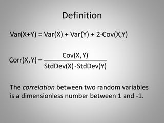
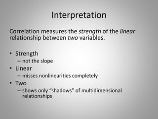
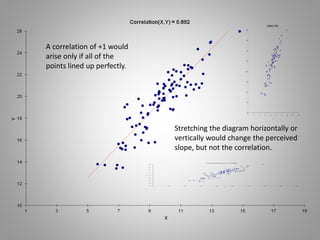
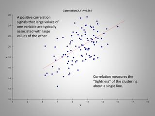
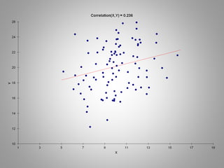
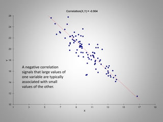
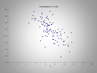
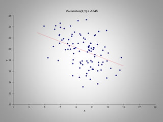
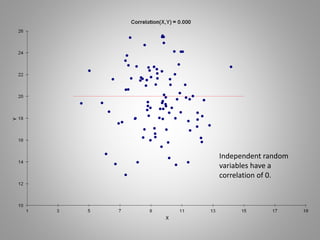
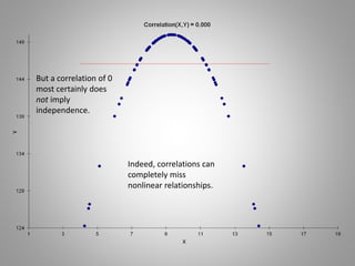
Correlation measures the strength of a linear relationship between two variables on a scale from -1 to 1. A correlation of 0 means there is no linear relationship, 1 means a perfect positive linear relationship, and -1 means a perfect negative linear relationship. Correlation only measures linear relationships and can miss nonlinear relationships. While correlation indicates association, it does not prove causation between the variables. Regression is needed to determine the relative weights and significance of predictors for a dependent variable.

1. Correlation
... beware

2. Definition
Var(X+Y) = Var(X) + Var(Y) + 2·Cov(X,Y)
The correlation between two random variables
is a dimensionless number between 1 and -1.
)
Y
(
StdDev
)
X
(
StdDev
)
Y
,
X
(
Cov
)
Y
,
X
(
Corr



3. Interpretation
Correlation measures the strength of the linear
relationship between two variables.
• Strength
– not the slope
• Linear
– misses nonlinearities completely
• Two
– shows only “shadows” of multidimensional
relationships

4. A correlation of +1 would
arise only if all of the
points lined up perfectly.
Stretching the diagram horizontally or
vertically would change the perceived
slope, but not the correlation.

5. Correlation measures the
“tightness” of the clustering
about a single line.
A positive correlation
signals that large values of
one variable are typically
associated with large
values of the other.

7. A negative correlation
signals that large values of
one variable are typically
associated with small
values of the other.

10. Independent random
variables have a
correlation of 0.

11. But a correlation of 0
most certainly does
not imply
independence.
Indeed, correlations can
completely miss
nonlinear relationships.

12. Correlations Show (only)
Two-Dimensional Shadows
In the motorpool case, the correlations between Age and Cost, and between
Make and Cost, show precisely what the manager’s two-dimensional tables
showed:
There’s little linkage directly between Age and Cost.
Fords had higher average costs than did Hondas.
But each of these facts is due to the confounding effect of Mileage!
The pure effect of each variable on its own is only revealed in the most-
complete model.
Costs Mileage Age Make
Costs 1.000 0.771 0.023 -0.240
Mileage 0.771 1.000 -0.496 -0.478
Age 0.023 -0.496 1.000 0.164
Make -0.240 -0.478 0.164 1.000

13. Tilting at Shadows
(received via email from a former student, all employer references
removed)
“One of the pieces of the research is to identify key attributes that
drive customers to choose a vendor for buying office products.
“The market research guy that we have hired (he is an MBA/PhD from
Wharton) says the following:
“‘I can determine the relative importance of various attributes that
drive overall satisfaction by running a correlation of each one of them
against overall satisfaction score and then ranking them based on the
(correlation) coefficient scores.’
“I am not really certain if we can do that. I would tend to think we
should run a regression to get relative weightage.”

14. Correlations with Satisfaction
leadtime -0.766
ol-tracking -0.242
cost 0.097
Customer Satisfaction
• Consider overall customer satisfaction (on a 100-point scale) with
a Web-based provider of customized software as the order
leadtime (in days), product acquisition cost, and availability of
online order-tracking (0 = not available, 1 = available) vary.
• Here are the correlations:
 Customers forced to wait are unhappy.
 Those without access to online order tracking are more satisfied.
 Those who pay more are somewhat happier.
 ?????

15. Regression: satisfaction constant leadtime cost ol-track
coefficient 192.7338 -6.8856 -1.8025 8.5599
std error of coef 16.1643 0.5535 0.3137 4.0729
t-ratio 11.9234 -12.4391 -5.7453 2.1017
significance 0.0000% 0.0000% 0.0000% 4.0092%
beta-weight -1.0879 -0.4571 0.1586
standard error of regression 13.9292
coefficient of determination 75.03%
adjusted coef of determination 73.70%
The Full Regression
Customers dislike high cost, and like online order tracking.
Why does customer satisfaction vary? Primarily because
leadtimes vary; secondarily, because cost varies.

16. Reconciliation
• Customers can pay extra for expedited service (shorter
leadtime at moderate extra cost), or for express service
(shortest leadtime at highest cost)
– Those who chose to save money and wait longer ended up
(slightly) regretting their choice.
• Most customers who chose rapid service weren’t given
access to order tracking.
– They didn’t need it, and were still happy with their fast
deliveries.
satisfaction leadtime cost ol-tracking
satisfaction 1.000 -0.766 -0.097 -0.242
leadtime -0.766 1.000 -0.543 0.465
cost -0.097 -0.543 1.000 -0.230
ol-tracking -0.242 0.465 -0.230 1.000

17. Finally …
• The correlations between the explanatory variables can help flesh out the
“story.”
• In a “simple” (i.e., one explanatory variable) regression:
– The (meaningless) beta-weight is the correlation between the two variables.
– The square of the correlation is the unadjusted coefficient of determination (r-
squared).
Regression: Costs
constant Mileage
coefficient 364.476942 19.812076
std error of coef 76.8173302 4.54471998
t-ratio 4.7447 4.3594
significance 0.0383% 0.0774%
beta-weight 0.7706
standard error of regression 73.8638412
coefficient of determination 59.38%
adjusted coef of determination 56.26%
If you give me a correlation, I’ll
interpret it by squaring it and
looking at it as a coefficient of
determination.

18. A Pharmaceutical Ad
Correlation(anxiety,depression) = 0.7
0
10
20
30
40
50
60
70
80
90
100
0 10 20 30 40 50 60 70 80 90 100
depression
anxiety
Diagnostic scores from sample of patients receiving psychiatric care
So, if your patients have anxiety problems, consider prescribing our antidepressant!

19. Evaluation
• At most 49% of the variability in patients’
anxiety levels can potentially be explained by
variability in depression levels.
– “potentially” = might actually be explained by
something else which covaries with both.
• The regression provides no evidence that
changing a patient’s depression level will
cause a change in their anxiety level.

20. Association vs. Causality
• Polio and Ice Cream
• Regression (and correlation) deal only with association
– Example: Greater values for annual mileage are typically
associated with higher annual maintenance costs.
– No matter how “good” the regression statistics look, they will
not make the case that greater mileage causes greater costs.
– If you believe that driving more during the year causes higher
costs, then it’s fine to use regression to estimate the size of the
causal effect.
• Evidence supporting causality comes only from controlled
experimentation.
– This is why macroeconomists continue to argue about which
aspects of public policy are the key drivers of economic growth.
– It’s also why the cigarette companies won all the lawsuits filed
against them for several decades.