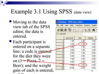
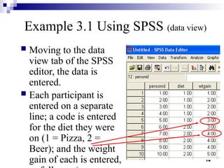
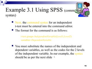
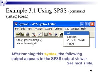
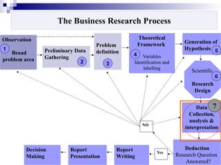
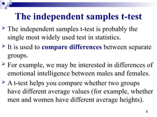
Business Research Process (Step-7):
Data Analysis &
Interpretation
Chapter 12
References:
• Research Methods For Business (Uma Sekaran)
• VU Book of BRM
• Business Research Methods (William G. Zikmund)
• Internet
The Business Research Process
Observation
Broad
problem area
Preliminary Data
Gathering
Problem
definition
Theoretical
Framework
Variables
Identification and
labelling
Generation of
Hypothesis
Scientific
Research
Design
Data
Collection,
analysis &
interpretation
Deduction
Research Question
Answered?
Report
Writing
Report
Presentation
Decision
Making
Yes
NO
1
2 3
4
5
6
7
3
The independent samples t-test
 The independent samples t-test is probably the
single most widely used test in statistics.
 It is used to compare differences between separate
groups.
 For example, we may be interested in differences of
emotional intelligence between males and females.
 A t-test helps you compare whether two groups
have different average values (for example, whether
men and women have different average heights).
4
When to use the independent samples t-test
 Any differences between groups can be explored
with the independent t-test, as long as the tested
members of each group are reasonably
representative of the population. [1]
[1] There are some technical
requirements as well. Principally,
each variable must come from a
normal (or nearly normal) distribution.
5
Example
 Suppose we put people on 2 diets:
the pizza diet and the beer diet.
 Participants are randomly assigned to either
1-week of eating exclusively pizza or 1-week
of exclusively drinking beer.
6
 At the end of the week, we measure
weight gain by each participant. Which diet causes
more weight gain?
 In other words, the null hypothesis is:
Ho: wt. gain pizza diet =wt. gain beer diet.
 The null hypothesis is the opposite of what we hope
to find.
 In this case, our research hypothesis is that there
ARE differences between the 2 diets.
 Therefore, our null hypothesis is that there are NO
differences between these 2 diets.
7
Some theory
 The “t” is calculated under the
assumption, called the null hypothesis,
that there are no differences between the
pizza and beer diet.
 If this were true, when we repeatedly
sample 10 people from the population and
put them in our 2 diets, most often we
would calculate a “t” of “0.”
8
Example Using SPSS
 First, the variables must be setup in the SPSS data editor.
 We need to include both the independent and dependent
variables.
 Although it is not strictly necessary, it is good practice to
give each person a unique code
(e.g., personid):
9
 In the previous example:
Dependent Variable
= wtgain (or weight gain)
Independent Variable = diet
 Why?
 The independent variable (diet) causes
changes in the dependent variable (weight
gain).
10
Example 3.1 Using SPSS (cont.)
 Next, we need to provide “codes” that
distinguish between the 2 types of diets.
 By clicking in the grey box of the “Label”
field in the row containing the “diet”
variable, we get a pop-up dialog that
allows us to code the diet variable.
 Arbitrarily, the pizza diet is coded as diet
“1” and the beer diet is diet “2.”
 Any other 2 codes would work, but these
suffice . See next slide.
11
Example 3.1 Using SPSS (coding)
12
Example 3.1 Using SPSS (data view)
 Moving to the data
view tab of the SPSS
editor, the data is
entered.
 Each participant is
entered on a separate
line; a code is entered
for the diet they were
on (1 = Pizza, 2 =
Beer); and the weight
gain of each is entered,
13
Example 3.1 Using SPSS (data view)
 Moving to the data
view tab of the SPSS
editor, the data is
entered.
 Each participant is
entered on a separate
line; a code is entered
for the diet they were
on (1 = Pizza, 2 =
Beer); and the weight
gain of each is entered,
14
Example 3.1 Using SPSS (data view)
 Moving to the data
view tab of the SPSS
editor, the data is
entered.
 Each participant is
entered on a separate
line; a code is entered
for the diet they were
on (1 = Pizza, 2 =
Beer); and the weight
gain of each is entered,
15
Example 3.1 Using SPSS (command
syntax)
 Next, the command syntax for an independent
t-test must be entered into the command editor.
 The format for the command is as follows:
t-test groups IndependentVariable(Level1,Level2)
variables=DependentVariable.
 You must substitute the names of the independent and
dependent variables, as well as the codes for the 2 levels
of the independent variable. In our example, the syntax
should be as per the next slide 
16
Example 3.1 Using SPSS (command
syntax) (cont.)
After running this syntax, the following
output appears in the SPSS output viewer
See next slide.
17
Example 3.1: SPSS Output viewer
Independent Samples Test
18
Example 3.1 Using SPSS (cont.)
 SPSS gives the means for each of the
conditions (Pizza Mean = 2 and Beer
Mean = 4).
 In addition, SPSS provides a t-value of -
4.47 with 8 degrees of freedom.
 These are the same figures that were
computed “by hand” previously.
 However, SPSS does not provide a critical
value.
 Instead, an exact probability is provided (p
19
Example 3.1 Using SPSS (cont.)
 As long as this p-value falls below the
standard of “.05,” we can declare a significant
difference between our mean values.
 Since “.002” is below “.05” we can conclude:
Participants on the Beer diet (M = 4.00) gained
significantly more weight than
those on the Pizza diet (M = 2.00),
t(8) = 4.47, p < .01 (two-tailed).
20
Example 3.1 Using SPSS (cont.)
Repeat from previous slide:
Participants on the Beer diet (M = 4.00) gained
significantly more weight than those on the Pizza diet (M
= 2.00), t(8) = 4.47,
p < .01 (two-tailed).
 In APA style we normally only
display significance to 2 significant digits.
 Therefore, the probability is displayed as
“p<.01,” which is the smallest probability
within this range of accuracy.
21
Example 3.1 Using SPSS (cont.)
 The SPSS output also displays Levene’s Test for
Equality of Variances (see the first 2 columns in second
table on slide 30).
 Why?
 Strictly speaking, the t-test is only valid if we have
approximately equal variances within each of our two
groups.
 In our example, this was not a problem because the 2
variances were exactly equal (Variance Pizza = 0.04 and
Variance Beer = 0.04).
22
Example 3.1 Using SPSS (cont.)
 However, if this test is significant, meaning
that the p-value given is less than “.05,” then
we should choose the bottom line when
interpreting our results.
 This bottom line makes slight adjustments to
the t-test to account
for problems when there are not
equal variances in both conditions.
23
Example 3.1 Using SPSS (cont.)
 The practical importance of this distinction is
small.
 Even if variances are not equal between
conditions, the hand calculations we have
shown will most often lead to the correct
conclusion anyway, and use of the “top line” is
almost always appropriate.
24
Independent Samples t-
Test (or 2-Sample t-Test)
Advanced Research Methods in Psychology
- Week 2 lecture -
Matthew Rockloff
12. Data  Analysis & Interpretation.pptx

12. Data Analysis & Interpretation.pptx

  • 1.
    Business Research Process(Step-7): Data Analysis & Interpretation Chapter 12 References: • Research Methods For Business (Uma Sekaran) • VU Book of BRM • Business Research Methods (William G. Zikmund) • Internet
  • 2.
    The Business ResearchProcess Observation Broad problem area Preliminary Data Gathering Problem definition Theoretical Framework Variables Identification and labelling Generation of Hypothesis Scientific Research Design Data Collection, analysis & interpretation Deduction Research Question Answered? Report Writing Report Presentation Decision Making Yes NO 1 2 3 4 5 6 7
  • 3.
    3 The independent samplest-test  The independent samples t-test is probably the single most widely used test in statistics.  It is used to compare differences between separate groups.  For example, we may be interested in differences of emotional intelligence between males and females.  A t-test helps you compare whether two groups have different average values (for example, whether men and women have different average heights).
  • 4.
    4 When to usethe independent samples t-test  Any differences between groups can be explored with the independent t-test, as long as the tested members of each group are reasonably representative of the population. [1] [1] There are some technical requirements as well. Principally, each variable must come from a normal (or nearly normal) distribution.
  • 5.
    5 Example  Suppose weput people on 2 diets: the pizza diet and the beer diet.  Participants are randomly assigned to either 1-week of eating exclusively pizza or 1-week of exclusively drinking beer.
  • 6.
    6  At theend of the week, we measure weight gain by each participant. Which diet causes more weight gain?  In other words, the null hypothesis is: Ho: wt. gain pizza diet =wt. gain beer diet.  The null hypothesis is the opposite of what we hope to find.  In this case, our research hypothesis is that there ARE differences between the 2 diets.  Therefore, our null hypothesis is that there are NO differences between these 2 diets.
  • 7.
    7 Some theory  The“t” is calculated under the assumption, called the null hypothesis, that there are no differences between the pizza and beer diet.  If this were true, when we repeatedly sample 10 people from the population and put them in our 2 diets, most often we would calculate a “t” of “0.”
  • 8.
    8 Example Using SPSS First, the variables must be setup in the SPSS data editor.  We need to include both the independent and dependent variables.  Although it is not strictly necessary, it is good practice to give each person a unique code (e.g., personid):
  • 9.
    9  In theprevious example: Dependent Variable = wtgain (or weight gain) Independent Variable = diet  Why?  The independent variable (diet) causes changes in the dependent variable (weight gain).
  • 10.
    10 Example 3.1 UsingSPSS (cont.)  Next, we need to provide “codes” that distinguish between the 2 types of diets.  By clicking in the grey box of the “Label” field in the row containing the “diet” variable, we get a pop-up dialog that allows us to code the diet variable.  Arbitrarily, the pizza diet is coded as diet “1” and the beer diet is diet “2.”  Any other 2 codes would work, but these suffice . See next slide.
  • 11.
    11 Example 3.1 UsingSPSS (coding)
  • 12.
    12 Example 3.1 UsingSPSS (data view)  Moving to the data view tab of the SPSS editor, the data is entered.  Each participant is entered on a separate line; a code is entered for the diet they were on (1 = Pizza, 2 = Beer); and the weight gain of each is entered,
  • 13.
    13 Example 3.1 UsingSPSS (data view)  Moving to the data view tab of the SPSS editor, the data is entered.  Each participant is entered on a separate line; a code is entered for the diet they were on (1 = Pizza, 2 = Beer); and the weight gain of each is entered,
  • 14.
    14 Example 3.1 UsingSPSS (data view)  Moving to the data view tab of the SPSS editor, the data is entered.  Each participant is entered on a separate line; a code is entered for the diet they were on (1 = Pizza, 2 = Beer); and the weight gain of each is entered,
  • 15.
    15 Example 3.1 UsingSPSS (command syntax)  Next, the command syntax for an independent t-test must be entered into the command editor.  The format for the command is as follows: t-test groups IndependentVariable(Level1,Level2) variables=DependentVariable.  You must substitute the names of the independent and dependent variables, as well as the codes for the 2 levels of the independent variable. In our example, the syntax should be as per the next slide 
  • 16.
    16 Example 3.1 UsingSPSS (command syntax) (cont.) After running this syntax, the following output appears in the SPSS output viewer See next slide.
  • 17.
    17 Example 3.1: SPSSOutput viewer Independent Samples Test
  • 18.
    18 Example 3.1 UsingSPSS (cont.)  SPSS gives the means for each of the conditions (Pizza Mean = 2 and Beer Mean = 4).  In addition, SPSS provides a t-value of - 4.47 with 8 degrees of freedom.  These are the same figures that were computed “by hand” previously.  However, SPSS does not provide a critical value.  Instead, an exact probability is provided (p
  • 19.
    19 Example 3.1 UsingSPSS (cont.)  As long as this p-value falls below the standard of “.05,” we can declare a significant difference between our mean values.  Since “.002” is below “.05” we can conclude: Participants on the Beer diet (M = 4.00) gained significantly more weight than those on the Pizza diet (M = 2.00), t(8) = 4.47, p < .01 (two-tailed).
  • 20.
    20 Example 3.1 UsingSPSS (cont.) Repeat from previous slide: Participants on the Beer diet (M = 4.00) gained significantly more weight than those on the Pizza diet (M = 2.00), t(8) = 4.47, p < .01 (two-tailed).  In APA style we normally only display significance to 2 significant digits.  Therefore, the probability is displayed as “p<.01,” which is the smallest probability within this range of accuracy.
  • 21.
    21 Example 3.1 UsingSPSS (cont.)  The SPSS output also displays Levene’s Test for Equality of Variances (see the first 2 columns in second table on slide 30).  Why?  Strictly speaking, the t-test is only valid if we have approximately equal variances within each of our two groups.  In our example, this was not a problem because the 2 variances were exactly equal (Variance Pizza = 0.04 and Variance Beer = 0.04).
  • 22.
    22 Example 3.1 UsingSPSS (cont.)  However, if this test is significant, meaning that the p-value given is less than “.05,” then we should choose the bottom line when interpreting our results.  This bottom line makes slight adjustments to the t-test to account for problems when there are not equal variances in both conditions.
  • 23.
    23 Example 3.1 UsingSPSS (cont.)  The practical importance of this distinction is small.  Even if variances are not equal between conditions, the hand calculations we have shown will most often lead to the correct conclusion anyway, and use of the “top line” is almost always appropriate.
  • 24.
    24 Independent Samples t- Test(or 2-Sample t-Test) Advanced Research Methods in Psychology - Week 2 lecture - Matthew Rockloff