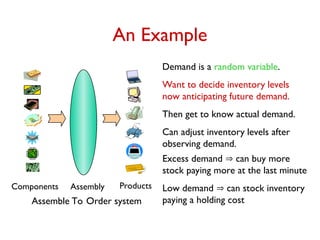
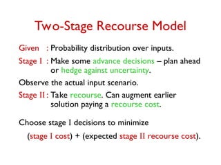
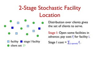
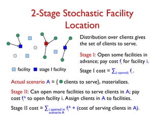
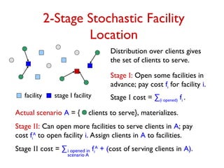
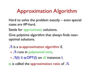
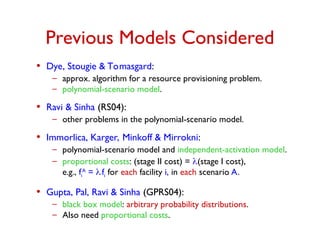
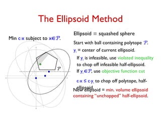
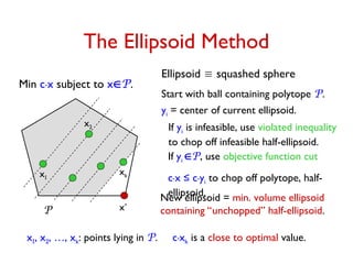
The document discusses stochastic optimization, focusing on modeling uncertainty in decision-making processes across various applications such as logistics and financial instruments. It presents a two-stage recourse model for inventory management and facility location problems and discusses approximation algorithms for stochastic integer optimization problems. Furthermore, it highlights methods to reduce stochastic optimization problems to their deterministic counterparts and presents results including approximation schemes for specific covering problems.

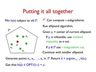
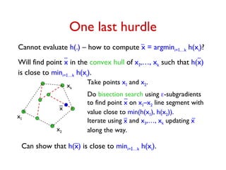
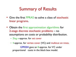
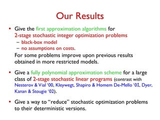
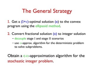
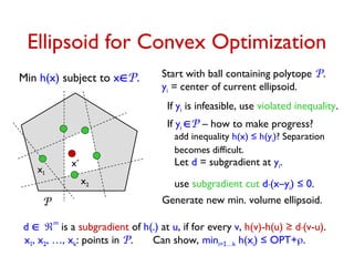
![Want to decide which facilities to open in stage I.
Goal: Minimize Total Cost =
(stage I cost) + EA D [stage II cost for A].
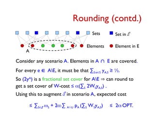
Two extremes:
1. Ultra-conservative: plan for “everything” and buy only
in stage I.
2. Defer all decisions to stage II.
Both strategies may be sub-optimal.
Want to prove a worst-case guarantee.
Give an algorithm that “works well” on any instance,
and for any probability distribution.](https://image.slidesharecdn.com/stochopt-long-241228185002-a93f5be6/85/stochopt-long-as-part-of-stochastic-optimization-9-320.jpg)
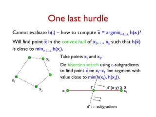
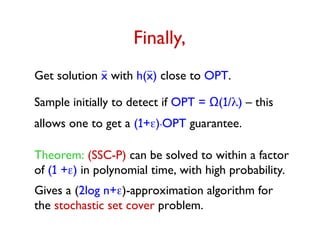
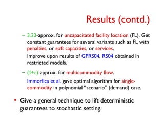
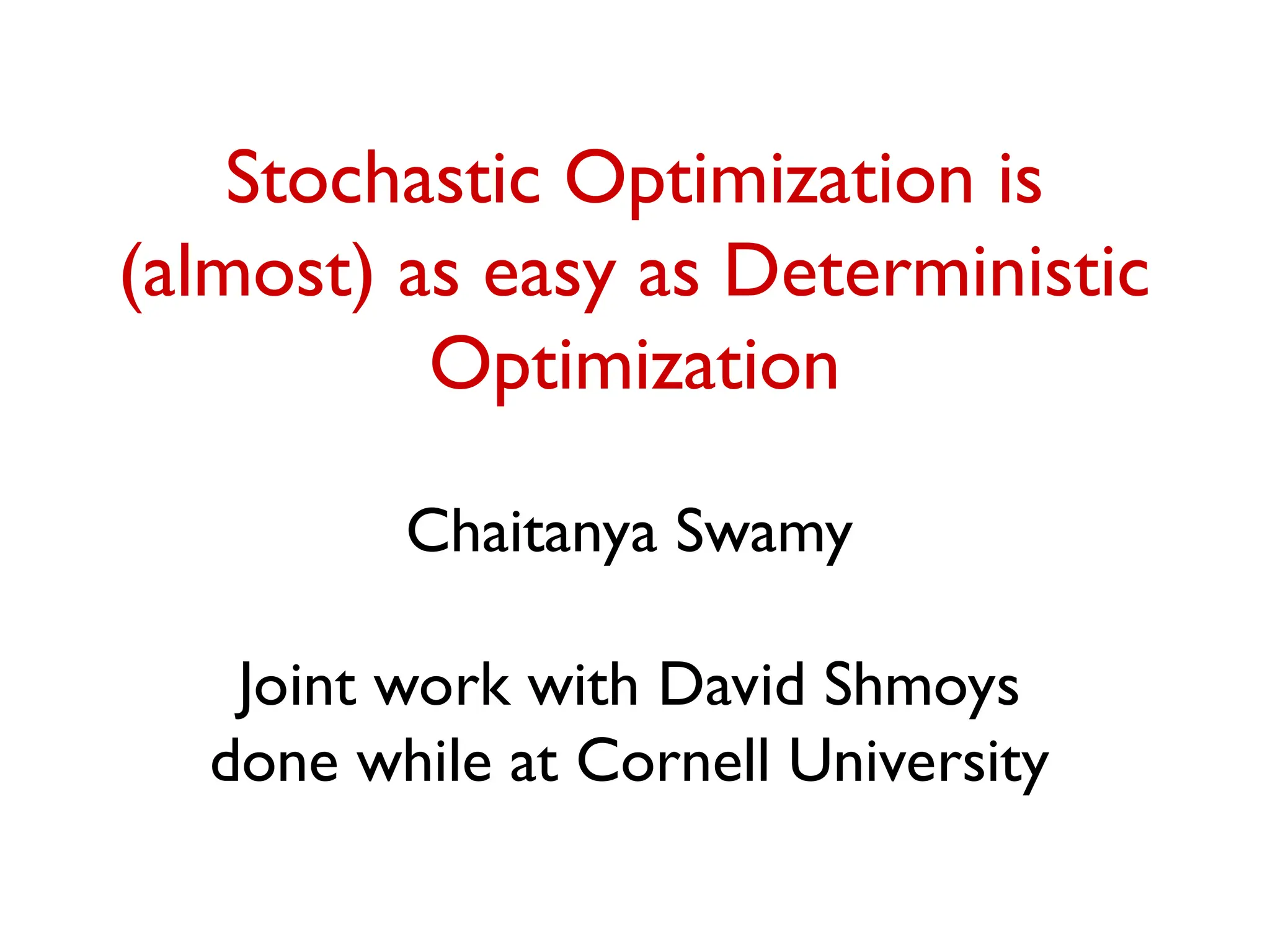
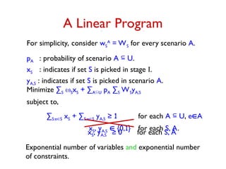
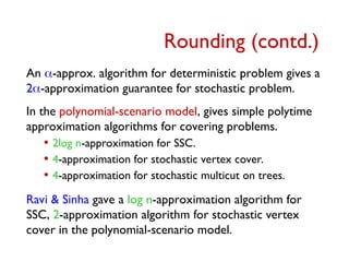
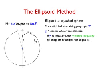
![Stochastic Set Cover (SSC)
Universe U = {e1, …, en }, subsets S1, S2, …, Sm
U, set S has
weight wS.
Deterministic problem: Pick a minimum weight collection of
sets that covers each element.
Stochastic version: Set of elements to be covered is given by
a probability distribution.
– choose some sets initially paying wS for set S
– subset A U to be covered is revealed
– can pick additional sets paying wS
A
for set S.
Minimize (w-cost of sets picked in stage I) +
EA U [wA
-cost of new sets picked for scenario A].](https://image.slidesharecdn.com/stochopt-long-241228185002-a93f5be6/85/stochopt-long-as-part-of-stochastic-optimization-13-320.jpg)
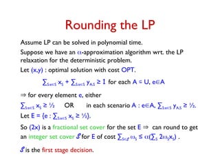
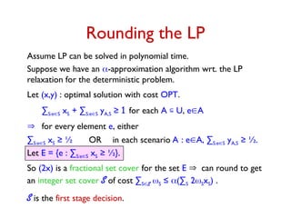
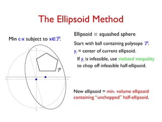
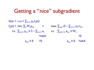
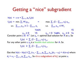
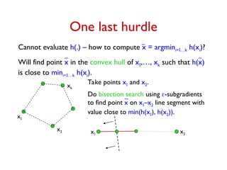
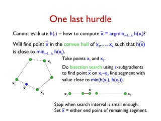
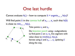
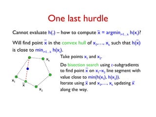
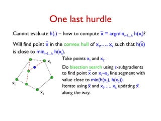
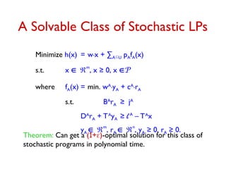
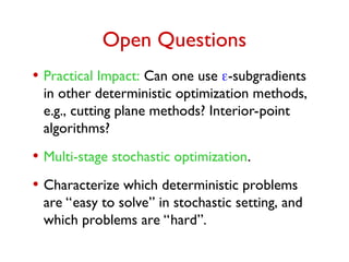
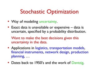
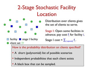
![Computing an -Subgradient
Given point u
m
. zA optimal dual solution for A at u.
Vector d with dS = S – ∑AU pA ∑eS zA,e
= ∑AU pA(S – ∑eS zA,e) is a subgradient at u.
Goal: Get d' such that dS – S ≤ d'S ≤ dS for each S.
For each S, -WS ≤ dS ≤ S. Let = maxS WS /S.
• Sample once from black box to get random scenario A.
Compute XS = S – ∑eS zA,e for each S.
E[XS] = dS and Var[XS] ≤ WS.
2
• Sample O(2
/2.log(m/)) times to compute d' such that
Pr[S, dS – S ≤ d'S ≤ dS] ≥ 1-
d' is an -subgradient at u with probability ≥ 1-](https://image.slidesharecdn.com/stochopt-long-241228185002-a93f5be6/85/stochopt-long-as-part-of-stochastic-optimization-35-320.jpg)