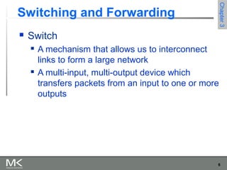
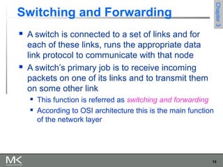
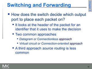
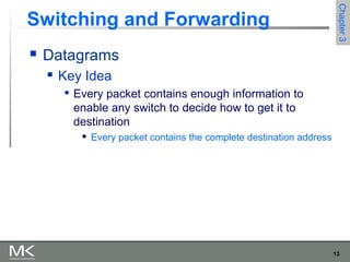
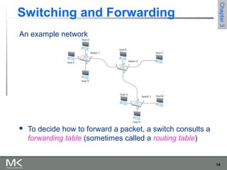
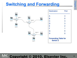
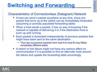
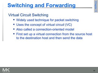
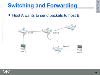
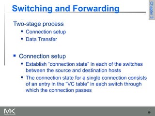
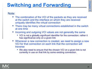
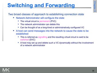
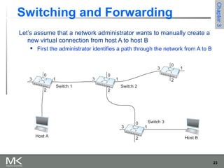
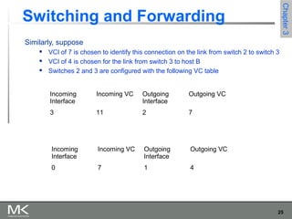
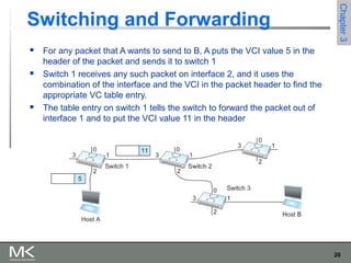
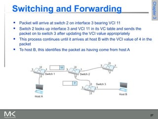
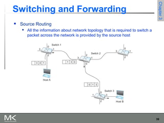
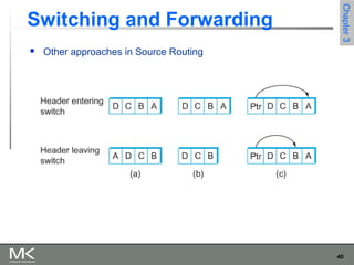
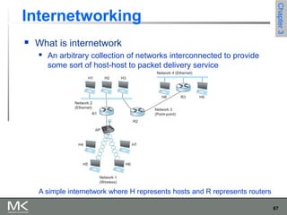
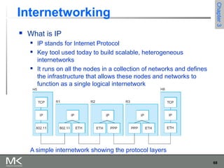
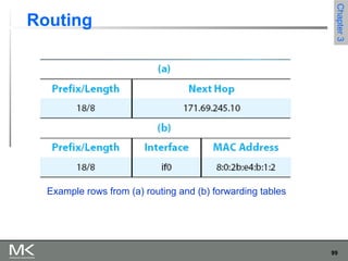
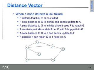
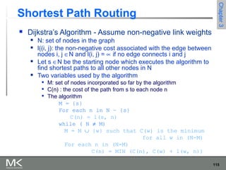
SlideShare a Scribd company logo
1 of 120
1
Chapter 3
Internetworking
Computer Networks: A Systems Approach, 5e
Larry L. Peterson and Bruce S. Davie
Copyright © 2010, Elsevier Inc. All rights Reserved
2
Chapter3Chapter3
Problems
 In Chapter 2 we saw how to connect one node to
another, or to an existing network. How do we
build networks of global scale?
 How do we interconnect different types of
networks to build a large global network?
3
Chapter3Chapter3
Chapter Outline
 Switching and Bridging
 Basic Internetworking (IP)
 Routing
4
Chapter3Chapter3
Chapter Goal
 Understanding the functions of switches, bridges
and routers
 Discussing Internet Protocol (IP) for
interconnecting networks
 Understanding the concept of routing
5
Chapter3Chapter3
Switching and Forwarding
 Store-and-Forward Switches
 Bridges and Extended LANs
 Cell Switching
 Segmentation and Reassembly
6
Chapter3Chapter3
Switching and Forwarding
 Switch
 A mechanism that allows us to interconnect
links to form a large network
 A multi-input, multi-output device which
transfers packets from an input to one or more
outputs
7
Chapter3Chapter3
Switching and Forwarding
Adds the star topology to the point-to-point link,
bus (Ethernet), and ring (802.5 and FDDI)
topologies
8
Chapter3Chapter3
Switching and Forwarding
Properties of this star topology
 Even though a switch has a fixed number of inputs and outputs,
which limits the number of hosts that can be connected to a
single switch, large networks can be built by interconnecting a
number of switches
 We can connect switches to each other and to hosts using point-
to-point links, which typically means that we can build networks
of large geographic scope
 Adding a new host to the network by connecting it to a switch
does not necessarily mean that the hosts already connected will
get worse performance from the network
9
Chapter3Chapter3
Switching and Forwarding
The last claim cannot be made for the shared
media network (discussed in Chapter 2)
 It is impossible for two hosts on the same Ethernet to
transmit continuously at 10Mbps because they share
the same transmission medium
 Every host on a switched network has its own link to
the switch

So it may be entirely possible for many hosts to transmit at
the full link speed (bandwidth) provided that the switch is
designed with enough aggregate capacity
10
Chapter3Chapter3
Switching and Forwarding
 A switch is connected to a set of links and for
each of these links, runs the appropriate data
link protocol to communicate with that node
 A switch’s primary job is to receive incoming
packets on one of its links and to transmit them
on some other link
 This function is referred as switching and forwarding
 According to OSI architecture this is the main function
of the network layer
11
Chapter3Chapter3
Switching and Forwarding
 How does the switch decide which output
port to place each packet on?
 It looks at the header of the packet for an
identifier that it uses to make the decision
 Two common approaches

Datagram or Connectionless approach

Virtual circuit or Connection-oriented approach
 A third approach source routing is less
common
12
Chapter3Chapter3
Switching and Forwarding
 Assumptions
 Each host has a globally unique address
 There is some way to identify the input and
output ports of each switch

We can use numbers

We can use names
13
Chapter3Chapter3
Switching and Forwarding
 Datagrams
 Key Idea

Every packet contains enough information to
enable any switch to decide how to get it to
destination
 Every packet contains the complete destination address
14
Chapter3Chapter3
An example network
 To decide how to forward a packet, a switch consults a
forwarding table (sometimes called a routing table)
Switching and Forwarding
15
Chapter3Chapter3
Copyright © 2010, Elsevier Inc.
Switching and Forwarding
Destination Port
-------------------------------------
A 3
B 0
C 3
D 3
E 2
F 1
G 0
H 0
Forwarding Table for
Switch 2
16
Chapter3Chapter3
Switching and Forwarding
Characteristics of Connectionless (Datagram) Network
 A host can send a packet anywhere at any time, since any
packet that turns up at the switch can be immediately forwarded
(assuming a correctly populated forwarding table)
 When a host sends a packet, it has no way of knowing if the
network is capable of delivering it or if the destination host is
even up and running
 Each packet is forwarded independently of previous packets that
might have been sent to the same destination.

Thus two successive packets from host A to host B may follow
completely different paths
 A switch or link failure might not have any serious effect on
communication if it is possible to find an alternate route around
the failure and update the forwarding table accordingly
17
Chapter3Chapter3
Switching and Forwarding
Virtual Circuit Switching
 Widely used technique for packet switching
 Uses the concept of virtual circuit (VC)
 Also called a connection-oriented model
 First set up a virtual connection from the source host
to the destination host and then send the data
18
Chapter3Chapter3
Switching and Forwarding
 Host A wants to send packets to host B
19
Chapter3Chapter3
Switching and Forwarding
Two-stage process
 Connection setup
 Data Transfer
 Connection setup
 Establish “connection state” in each of the switches
between the source and destination hosts
 The connection state for a single connection consists
of an entry in the “VC table” in each switch through
which the connection passes
20
Chapter3Chapter3
Switching and Forwarding
One entry in the VC table on a single switch contains
 A virtual circuit identifier (VCI) that uniquely identifies the connection at
this switch and that will be carried inside the header of the packets that
belong to this connection
 An incoming interface on which packets for this VC arrive at the switch
 An outgoing interface in which packets for this VC leave the switch
 A potentially different VCI that will be used for outgoing packets
 The semantics for one such entry is
 If a packet arrives on the designated incoming interface and that packet
contains the designated VCI value in its header, then the packet should
be sent out the specified outgoing interface with the specified outgoing
VCI value first having been placed in its header
21
Chapter3Chapter3
Switching and Forwarding
Note:
 The combination of the VCI of the packets as they are received
at the switch and the interface on which they are received
uniquely identifies the virtual connection
 There may be many virtual connections established in the switch
at one time
 Incoming and outgoing VCI values are not generally the same

VCI is not a globally significant identifier for the connection; rather it
has significance only on a given link
 Whenever a new connection is created, we need to assign a new
VCI for that connection on each link that the connection will
traverse

We also need to ensure that the chosen VCI on a given link is not
currently in use on that link by some existing connection.
22
Chapter3Chapter3
Switching and Forwarding
Two broad classes of approach to establishing connection state
 Network Administrator will configure the state

The virtual circuit is permanent (PVC)

The network administrator can delete this

Can be thought of as a long-lived or administratively configured VC
 A host can send messages into the network to cause the state to be
established

This is referred as signalling and the resulting virtual circuit is said to be
switched (SVC)

A host may set up and delete such a VC dynamically without the involvement
of a network administrator
23
Chapter3Chapter3
Let’s assume that a network administrator wants to manually create a
new virtual connection from host A to host B
 First the administrator identifies a path through the network from A to B
Switching and Forwarding
24
Chapter3Chapter3
Switching and Forwarding
The administrator then picks a VCI value that is currently unused on
each link for the connection
 For our example,

Suppose the VCI value 5 is chosen for the link from host A to switch 1

11 is chosen for the link from switch 1 to switch 2

So the switch 1 will have an entry in the VC table
Incoming
Interface
Incoming VC Outgoing
Interface
Outgoing VC
2 5 1 11
25
Chapter3Chapter3
Switching and Forwarding
Similarly, suppose
 VCI of 7 is chosen to identify this connection on the link from switch 2 to switch 3
 VCI of 4 is chosen for the link from switch 3 to host B
 Switches 2 and 3 are configured with the following VC table
Incoming
Interface
Incoming VC Outgoing
Interface
Outgoing VC
3 11 2 7
Incoming
Interface
Incoming VC Outgoing
Interface
Outgoing VC
0 7 1 4
26
Chapter3Chapter3
Switching and Forwarding
 For any packet that A wants to send to B, A puts the VCI value 5 in the
header of the packet and sends it to switch 1
 Switch 1 receives any such packet on interface 2, and it uses the
combination of the interface and the VCI in the packet header to find the
appropriate VC table entry.
 The table entry on switch 1 tells the switch to forward the packet out of
interface 1 and to put the VCI value 11 in the header
27
Chapter3Chapter3
Switching and Forwarding
 Packet will arrive at switch 2 on interface 3 bearing VCI 11
 Switch 2 looks up interface 3 and VCI 11 in its VC table and sends the
packet on to switch 3 after updating the VCI value appropriately
 This process continues until it arrives at host B with the VCI value of 4 in the
packet
 To host B, this identifies the packet as having come from host A
28
Chapter3Chapter3
Switching and Forwarding
 In real networks of reasonable size, the burden of configuring VC
tables correctly in a large number of switches would quickly become
excessive
 Thus, some sort of signalling is almost always used, even when setting
up “permanent” VCs
 In case of PVCs, signalling is initiated by the network administrator
 SVCs are usually set up using signalling by one of the hosts
29
Chapter3Chapter3
Switching and Forwarding
 How does the signalling work
 To start the signalling process, host A sends a setup message into the
network (i.e. to switch 1)

The setup message contains (among other things) the complete destination
address of B.

The setup message needs to get all the way to B to create the necessary
connection state in every switch along the way

It is like sending a datagram to B where every switch knows which output to
send the setup message so that it eventually reaches B
 Assume that every switch knows the topology to figure out how to do that
 When switch 1 receives the connection request, in addition to sending it
on to switch 2, it creates a new entry in its VC table for this new
connection

The entry is exactly the same shown in the previous table

Switch 1 picks the value 5 for this connection
30
Chapter3Chapter3
Switching and Forwarding
 How does the signalling work (contd.)
 When switch 2 receives the setup message, it performs the similar
process and it picks the value 11 as the incoming VCI
 Similarly switch 3 picks 7 as the value for its incoming VCI

Each switch can pick any number it likes, as long as that number is not
currently in use for some other connection on that port of that switch
 Finally the setup message arrives at host B.
 Assuming that B is healthy and willing to accept a connection from host
A, it allocates an incoming VCI value, in this case 4.

This VCI value can be used by B to identify all packets coming from A
31
Chapter3Chapter3
Switching and Forwarding
 Now to complete the connection, everyone needs to be told what
their downstream neighbor is using as the VCI for this connection
 Host B sends an acknowledgement of the connection setup to switch 3
and includes in that message the VCI value that it chose (4)
 Switch 3 completes the VC table entry for this connection and sends the
acknowledgement on to switch 2 specifying the VCI of 7
 Switch 2 completes the VC table entry for this connection and sends
acknowledgement on to switch 1 specifying the VCI of 11
 Finally switch 1 passes the acknowledgement on to host A telling it to
use the VCI value of 5 for this connection
32
Chapter3Chapter3
Switching and Forwarding
 When host A no longer wants to send data to host B, it tears down
the connection by sending a teardown message to switch 1
 The switch 1 removes the relevant entry from its table and forwards
the message on to the other switches in the path which similarly
delete the appropriate table entries
 At this point, if host A were to send a packet with a VCI of 5 to switch
1, it would be dropped as if the connection had never existed
33
Chapter3Chapter3
Switching and Forwarding
 Characteristics of VC
 Since host A has to wait for the connection request to reach the far side
of the network and return before it can send its first data packet, there is
at least one RTT of delay before data is sent
 While the connection request contains the full address for host B (which
might be quite large, being a global identifier on the network), each data
packet contains only a small identifier, which is only unique on one link.

Thus the per-packet overhead caused by the header is reduced relative to
the datagram model
 If a switch or a link in a connection fails, the connection is broken and a
new one will need to be established.

Also the old one needs to be torn down to free up table storage space in the
switches
 The issue of how a switch decides which link to forward the connection
request on has similarities with the function of a routing algorithm
34
Chapter3Chapter3
Copyright © 2010, Elsevier Inc.
Switching and Forwarding
 Good Properties of VC
 By the time the host gets the go-ahead to send data, it knows quite a lot
about the network-

For example, that there is really a route to the receiver and that the receiver
is willing to receive data
 It is also possible to allocate resources to the virtual circuit at the time it
is established
35
Chapter3Chapter3
Switching and Forwarding
 For example, an X.25 network – a packet-switched network that
uses the connection-oriented model – employs the following three-
part strategy
 Buffers are allocated to each virtual circuit when the circuit is initialized
 The sliding window protocol is run between each pair of nodes along the
virtual circuit, and this protocol is augmented with the flow control to
keep the sending node from overrunning the buffers allocated at the
receiving node
 The circuit is rejected by a given node if not enough buffers are available
at that node when the connection request message is processed
36
Chapter3Chapter3
Switching and Forwarding
 Comparison with the Datagram Model
 Datagram network has no connection establishment phase and each
switch processes each packet independently
 Each arriving packet competes with all other packets for buffer space
 If there are no buffers, the incoming packet must be dropped
 In VC, we could imagine providing each circuit with a different quality
of service (QoS)
 The network gives the user some kind of performance related guarantee

Switches set aside the resources they need to meet this guarantee
 For example, a percentage of each outgoing link’s bandwidth
 Delay tolerance on each switch
 Most popular examples of VC technologies are Frame Relay and
ATM
 One of the applications of Frame Relay is the construction of VPN
37
Chapter3Chapter3
Switching and Forwarding
 ATM (Asynchronous Transfer Mode)
 Connection-oriented packet-switched network
 Packets are called cells

5 byte header + 48 byte payload
 Fixed length packets are easier to switch in
hardware

Simpler to design

Enables parallelism
38
Chapter3Chapter3
Switching and Forwarding
 ATM
 User-Network Interface (UNI)

Host-to-switch format

GFC: Generic Flow Control

VCI: Virtual Circuit Identifier

Type: management, congestion control

CLP: Cell Loss Priority

HEC: Header Error Check (CRC-8)
 Network-Network Interface (NNI)

Switch-to-switch format

GFC becomes part of VPI field
39
Chapter3Chapter3
Switching and Forwarding
 Source Routing
 All the information about network topology that is required to switch a
packet across the network is provided by the source host
40
Chapter3Chapter3
Switching and Forwarding
 Other approaches in Source Routing
41
Chapter3Chapter3
Introduction to Congestion
• Contention – The queuing of multiple
packets at an output port of a switch
because they arrived at similar times. The
effect is delay of the packet arriving at the
output port while the port is busy.
• Congestion – The next stage of
contention, where the buffers used to store
contending packets are used up, requiring
dropping of packets.
• See shaded box on Page 182
42
Chapter3Chapter3
Optical Switching
• DWDM-Dense Wavelength Division Multiplexing
• Multiple wavelengths(colors) on single fiber
• ex: 100 channels of 10Gbps each
• Optical Amplifiers
• Old repeater spacing (back to electric) ~ 40Km
• DWDM equipment required at each repeater
• With Amplifiers 100’s of Km possible
• Optical Switches
• Current technology electrically ‘forward’ SONET channels
• Emerging technology using micro-mirror manipulation
• See shaded box on page 183
43
Chapter3Chapter3
First Network Switch
IMP1: The
first node of
the ARPANET
wirh Len
Kleinrock
circa 1969
http://www.lk.cs.ucla.edu/LK/Inet/birth.html
44
Chapter3Chapter3
Bridges and LAN Switches
 Bridges and LAN Switches
 Class of switches that is used to forward packets between shared-media
LANs such as Ethernets

Known as LAN switches

Referred to as Bridges
 Suppose you have a pair of Ethernets that you want to interconnect

One approach is put a repeater in between them
 It might exceed the physical limitation of the Ethernet

No more than four repeaters between any pair of hosts

No more than a total of 2500 m in length is allowed

An alternative would be to put a node between the two Ethernets and have
the node forward frames from one Ethernet to the other
 This node is called a Bridge
 A collection of LANs connected by one or more bridges is usually said to form an
Extended LAN
45
Chapter3Chapter3
Bridges and LAN Switches
 Simplest Strategy for Bridges
 Accept LAN frames on their inputs and forward them out to all other
outputs
 Used by early bridges
 Learning Bridges
 Observe that there is no need to forward all the frames that a bridge
receives
46
Chapter3Chapter3
 Consider the following figure
 When a frame from host A that is addressed to host B arrives on port 1,
there is no need for the bridge to forward the frame out over port 2.
 How does a bridge come to learn on which port the various hosts
reside?
Bridges and LAN Switches
47
Chapter3Chapter3
Bridges and LAN Switches
 Solution
 Download a table into the bridge
 Who does the download?

Human
 Too much work for maintenance
A
Bridge
B C
X Y Z
Port 1
Port 2
Host Port
--------------------
A 1
B 1
C 1
X 2
Y 2
Z 2
48
Chapter3Chapter3
Bridges and LAN Switches
 Can the bridge learn this information by itself?
 Yes
 How
 Each bridge inspects the source address in all the frames it receives
 Record the information at the bridge and build the table
 When a bridge first boots, this table is empty
 Entries are added over time
 A timeout is associated with each entry
 The bridge discards the entry after a specified period of time

To protect against the situation in which a host is moved from one network to
another
 If the bridge receives a frame that is addressed to host not currently
in the table
 Forward the frame out on all other ports
49
Chapter3Chapter3
Bridges and LAN Switches
 Strategy works fine if the extended LAN does not have a loop in it
 Why?
 Frames potentially loop through the extended LAN forever
 Bridges B1, B4, and B6 form a loop
50
Chapter3Chapter3
Bridges and LAN Switches
 How does an extended LAN come to have a loop in it?
 Network is managed by more than one administrator

For example, it spans multiple departments in an organization

It is possible that no single person knows the entire configuration of
the network
 A bridge that closes a loop might be added without anyone knowing
 Loops are built into the network to provide redundancy in case of
failures
 Solution
 Distributed Spanning Tree Algorithm
51
Chapter3Chapter3
Spanning Tree Algorithm
 Think of the extended LAN as being represented by a graph that
possibly has loops (cycles)
 A spanning tree is a sub-graph of this graph that covers
all the vertices but contains no cycles
 Spanning tree keeps all the vertices of the original graph but
throws out some of the edges
Example of (a) a cyclic graph; (b) a corresponding spanning tree.
52
Chapter3Chapter3
Spanning Tree Algorithm
 Developed by Radia Perlman at Digital
 A protocol used by a set of bridges to agree upon a spanning
tree for a particular extended LAN
 IEEE 802.1 specification for LAN bridges is based on this
algorithm
 Each bridge decides the ports over which it is and is not willing to
forward frames

In a sense, it is by removing ports from the topology that the
extended LAN is reduced to an acyclic tree

It is even possible that an entire bridge will not participate in
forwarding frames
53
Chapter3Chapter3
Spanning Tree Algorithm
 Algorithm is dynamic
 The bridges are always prepared to reconfigure themselves into
a new spanning tree if some bridges fail
 Main idea
 Each bridge selects the ports over which they will forward the
frames
54
Chapter3Chapter3
Spanning Tree Algorithm
 Algorithm selects ports as follows:
 Each bridge has a unique identifier

B1, B2, B3,…and so on.
 Elect the bridge with the smallest id as the root of the spanning
tree
 The root bridge always forwards frames out over all of its ports
 Each bridge computes the shortest path to the root and notes
which of its ports is on this path

This port is selected as the bridge’s preferred path to the root
 Finally, all the bridges connected to a given LAN elect a single
designated bridge that will be responsible for forwarding frames
toward the root bridge
55
Chapter3Chapter3
Spanning Tree Algorithm
 Each LAN’s designated bridge is the one that is closest to the root
 If two or more bridges are equally close to the root,
 Then select bridge with the smallest id
 Each bridge is connected to more than one LAN
 So it participates in the election of a designated bridge for each LAN it is
connected to.
 Each bridge decides if it is the designated bridge relative to each of its
ports
 The bridge forwards frames over those ports for which it is the
designated bridge
56
Chapter3Chapter3
Spanning Tree Algorithm
 B1 is the root bridge
 B3 and B5 are connected to LAN A, but B5 is the designated bridge
 B5 and B7 are connected to LAN B, but B5 is the designated bridge
57
Chapter3Chapter3
Spanning Tree Algorithm
 Initially each bridge thinks it is the root, so it sends a configuration
message on each of its ports identifying itself as the root and giving
a distance to the root of 0
 Upon receiving a configuration message over a particular port, the
bridge checks to see if the new message is better than the current
best configuration message recorded for that port
 The new configuration is better than the currently recorded
information if
 It identifies a root with a smaller id or
 It identifies a root with an equal id but with a shorter distance or
 The root id and distance are equal, but the sending bridge has a smaller
id
58
Chapter3Chapter3
Spanning Tree Algorithm
 If the new message is better than the currently recorded one,
 The bridge discards the old information and saves the new information
 It first adds 1 to the distance-to-root field
 When a bridge receives a configuration message indicating that it is
not the root bridge (that is, a message from a bridge with smaller id)
 The bridge stops generating configuration messages on its own
 Only forwards configuration messages from other bridges after 1 adding
to the distance field
59
Chapter3Chapter3
Spanning Tree Algorithm
 When a bridge receives a configuration message that indicates it is
not the designated bridge for that port
=> a message from a bridge that is closer to the root or equally far from the
root but with a smaller id

The bridge stops sending configuration messages over that port
 When the system stabilizes,
 Only the root bridge is still generating configuration messages.
 Other bridges are forwarding these messages only over ports for which
they are the designated bridge
60
Chapter3Chapter3
Spanning Tree Algorithm
 Consider the situation when the power had just been restored to the
building housing the following network
 All bridges would start off by claiming to be the root
61
Chapter3Chapter3
Spanning Tree Algorithm
 Denote a configuration message from node X in which it claims to be
distance d from the root node Y as (Y, d, X)
 Consider the activity at node B3
62
Chapter3Chapter3
Spanning Tree Algorithm
 B3 receives (B2, 0, B2)
 Since 2 < 3, B3 accepts B2 as root
 B3 adds 1 to the distance advertised
by B2 and sends (B2, 1, B3) to B5
 Meanwhile B2 accepts B1 as root
because it has the lower id and it
sends (B1, 1, B2) toward B3
 B5 accepts B1 as root and sends (B1,
1, B5) to B3
 B3 accepts B1 as root and it notes
that both B2 and B5 are closer to the
root than it is.
 Thus B3 stops forwarding messages
on both its interfaces
 This leaves B3 with both ports not
selected
63
Chapter3Chapter3
Spanning Tree Algorithm
 Even after the system has stabilized, the root bridge continues to
send configuration messages periodically
 Other bridges continue to forward these messages
 When a bridge fails, the downstream bridges will not receive the
configuration messages
 After waiting a specified period of time, they will once again claim to
be the root and the algorithm starts again
 Note
 Although the algorithm is able to reconfigure the spanning tree whenever
a bridge fails, it is not able to forward frames over alternative paths for
the sake of routing around a congested bridge
64
Chapter3Chapter3
Spanning Tree Algorithm
 Broadcast and Multicast
 Forward all broadcast/multicast frames

Current practice
 Learn when no group members downstream
 Accomplished by having each member of
group G send a frame to bridge multicast
address with G in source field
65
Chapter3Chapter3
Spanning Tree Algorithm
 Limitation of Bridges
 Do not scale

Spanning tree algorithm does not scale

Broadcast does not scale
 Do not accommodate heterogeneity
 Caution: Beware of Transparency
66
Chapter3Chapter3
Spanning Tree Algorithm
 Virtual LAN
67
Chapter3Chapter3
Internetworking
 What is internetwork
 An arbitrary collection of networks interconnected to provide
some sort of host-host to packet delivery service
A simple internetwork where H represents hosts and R represents routers
68
Chapter3Chapter3
Internetworking
 What is IP
 IP stands for Internet Protocol
 Key tool used today to build scalable, heterogeneous
internetworks
 It runs on all the nodes in a collection of networks and defines
the infrastructure that allows these nodes and networks to
function as a single logical internetwork
A simple internetwork showing the protocol layers
69
Chapter3Chapter3
IP Service Model
 Packet Delivery Model
 Connectionless model for data delivery
 Best-effort delivery (unreliable service)

packets are lost

packets are delivered out of order

duplicate copies of a packet are delivered

packets can be delayed for a long time
 Global Addressing Scheme
 Provides a way to identify all hosts in the network
70
Chapter3Chapter3
Packet Format
 Version (4): currently 4
 Hlen (4): number of 32-bit words
in header
 TOS (8): type of service (not
widely used)
 Length (16): number of bytes in
this datagram
 Ident (16): used by fragmentation
 Flags/Offset (16): used by
fragmentation
 TTL (8): number of hops this
datagram has traveled
 Protocol (8): demux key (TCP=6,
UDP=17)
 Checksum (16): of the header
only
 DestAddr & SrcAddr (32)
71
Chapter3Chapter3
IP Fragmentation and Reassembly
 Each network has some MTU (Maximum
Transmission Unit)
 Ethernet (1500 bytes), FDDI (4500 bytes)
 Strategy
 Fragmentation occurs in a router when it receives a
datagram that it wants to forward over a network
which has (MTU < datagram)
 Reassembly is done at the receiving host
 All the fragments carry the same identifier in the Ident
field
 Fragments are self-contained datagrams
 IP does not recover from missing fragments
72
Chapter3Chapter3
IP Fragmentation and Reassembly
IP datagrams traversing the sequence of physical networks
73
Chapter3Chapter3
IP Fragmentation and Reassembly
Header fields used in IP fragmentation. (a) Unfragmented packet; (b) fragmented packets.
74
Chapter3Chapter3
Global Addresses
 Properties
 globally unique
 hierarchical: network + host
 4 Billion IP address, half are A type, ¼ is B type, and 1/8 is C
type
 Format
 Dot notation
 10.3.2.4
 128.96.33.81
 192.12.69.77
75
Chapter3Chapter3
IP Datagram Forwarding
 Strategy
 every datagram contains destination's address
 if directly connected to destination network, then forward to host
 if not directly connected to destination network, then forward to
some router
 forwarding table maps network number into next hop
 each host has a default router
 each router maintains a forwarding table
 Example (router R2)
76
Chapter3Chapter3
IP Datagram Forwarding
 Algorithm
if (NetworkNum of destination = NetworkNum of one of my
interfaces) then
deliver packet to destination over that interface
else
if (NetworkNum of destination is in my forwarding table)
then
deliver packet to NextHop router
else
deliver packet to default router
For a host with only one interface and only a default router in its forwarding
table, this simplifies to
if (NetworkNum of destination = my NetworkNum)then
deliver packet to destination directly
else
deliver packet to default router
77
Chapter3Chapter3
Subnetting
 Add another level to address/routing hierarchy: subnet
 Subnet masks define variable partition of host part of
class A and B addresses
 Subnets visible only within site
78
Chapter3Chapter3
Subnetting
 Forwarding Table at Router R1
79
Chapter3Chapter3
Subnetting
Forwarding Algorithm
D = destination IP address
for each entry < SubnetNum, SubnetMask, NextHop>
D1 = SubnetMask & D
if D1 = SubnetNum
if NextHop is an interface
deliver datagram directly to destination
else
deliver datagram to NextHop (a router)
80
Chapter3Chapter3
Subnetting
Notes
 Would use a default router if nothing matches
 Not necessary for all ones in subnet mask to be
contiguous
 Can put multiple subnets on one physical network
 Subnets not visible from the rest of the Internet
81
Chapter3Chapter3
Classless Addressing
 Classless Inter-Domain Routing
 A technique that addresses two scaling concerns in
the Internet

The growth of backbone routing table as more and more
network numbers need to be stored in them

Potential exhaustion of the 32-bit address space
 Address assignment efficiency

Arises because of the IP address structure with class A, B,
and C addresses

Forces us to hand out network address space in fixed-size
chunks of three very different sizes
 A network with two hosts needs a class C address

Address assignment efficiency = 2/255 = 0.78
 A network with 256 hosts needs a class B address

Address assignment efficiency = 256/65535 = 0.39
82
Chapter3Chapter3
Classless Addressing
 Exhaustion of IP address space centers on exhaustion of
the class B network numbers
 Solution
 Say “NO” to any Autonomous System (AS) that requests a class
B address unless they can show a need for something close to
64K addresses
 Instead give them an appropriate number of class C addresses
 For any AS with at least 256 hosts, we can guarantee an address
space utilization of at least 50%
 What is the problem with this solution?
83
Chapter3Chapter3
Classless Addressing
 Problem with this solution
 Excessive storage requirement at the routers.
 If a single AS has, say 16 class C network
numbers assigned to it,
 Every Internet backbone router needs 16 entries in its
routing tables for that AS
 This is true, even if the path to every one of these
networks is the same
 If we had assigned a class B address to the AS
 The same routing information can be stored in one
entry
 Efficiency = 16 × 255 / 65, 536 = 6.2%
84
Chapter3Chapter3
Classless Addressing
 CIDR tries to balance the desire to minimize the
number of routes that a router needs to know
against the need to hand out addresses
efficiently.
 CIDR uses aggregate routes
 Uses a single entry in the forwarding table to tell the
router how to reach a lot of different networks
 Breaks the rigid boundaries between address classes
85
Chapter3Chapter3
Classless Addressing
 Consider an AS with 16 class C network numbers.
 Instead of handing out 16 addresses at random, hand
out a block of contiguous class C addresses
 Suppose we assign the class C network numbers from
192.4.16 through 192.4.31
 Observe that top 20 bits of all the addresses in this range
are the same (11000000 00000100 0001)
 We have created a 20-bit network number (which is in between
class B network number and class C number)
 Requires to hand out blocks of class C addresses that
share a common prefix
86
Chapter3Chapter3
Classless Addressing
 Requires to hand out blocks of class C addresses that
share a common prefix
 The convention is to place a /X after the prefix where X is
the prefix length in bits
 For example, the 20-bit prefix for all the networks
192.4.16 through 192.4.31 is represented as 192.4.16/20
 By contrast, if we wanted to represent a single class C
network number, which is 24 bits long, we would write it
192.4.16/24
87
Chapter3Chapter3
Classless Addressing
 How do the routing protocols handle this
classless addresses
 It must understand that the network number may be of
any length
 Represent network number with a single pair
<length, value>
 All routers must understand CIDR addressing
88
Chapter3Chapter3
Classless Addressing
Route aggregation with CIDR
89
Chapter3Chapter3
IP Forwarding Revisited
 IP forwarding mechanism assumes that it can
find the network number in a packet and then
look up that number in the forwarding table
 We need to change this assumption in case of
CIDR
 CIDR means that prefixes may be of any length,
from 2 to 32 bits
90
Chapter3Chapter3
IP Forwarding Revisited
 It is also possible to have prefixes in the forwarding
tables that overlap
 Some addresses may match more than one prefix
 For example, we might find both 171.69 (a 16 bit prefix)
and 171.69.10 (a 24 bit prefix) in the forwarding table of a
single router
 A packet destined to 171.69.10.5 clearly matches both
prefixes.
 The rule is based on the principle of “longest match”

171.69.10 in this case
 A packet destined to 171.69.20.5 would match 171.69
and not 171.69.10
91
Chapter3Chapter3
Address Translation Protocol (ARP)
 Map IP addresses into physical addresses
 destination host
 next hop router
 Techniques
 encode physical address in host part of IP address
 table-based
 ARP (Address Resolution Protocol)
 table of IP to physical address bindings
 broadcast request if IP address not in table
 target machine responds with its physical address
 table entries are discarded if not refreshed
92
Chapter3Chapter3
ARP Packet Format
 HardwareType: type of physical network (e.g., Ethernet)
 ProtocolType: type of higher layer protocol (e.g., IP)
 HLEN & PLEN: length of physical and protocol addresses
 Operation: request or response
 Source/Target Physical/Protocol addresses
93
Chapter3Chapter3
Host Configurations
 Notes
 Ethernet addresses are configured into network by
manufacturer and they are unique
 IP addresses must be unique on a given internetwork
but also must reflect the structure of the internetwork
 Most host Operating Systems provide a way to
manually configure the IP information for the host
 Drawbacks of manual configuration

A lot of work to configure all the hosts in a large network

Configuration process is error-prune
 Automated Configuration Process is required
94
Chapter3Chapter3
Dynamic Host Configuration Protocol (DHCP)
 DHCP server is responsible for providing
configuration information to hosts
 There is at least one DHCP server for an
administrative domain
 DHCP server maintains a pool of available
addresses
95
Chapter3Chapter3
DHCP
 Newly booted or
attached host sends
DHCPDISCOVER
message to a special IP
address
(255.255.255.255)
 DHCP relay agent
unicasts the message to
DHCP server and waits
for the response
96
Chapter3Chapter3
Internet Control Message Protocol (ICMP)
 Defines a collection of error messages that are sent back
to the source host whenever a router or host is unable to
process an IP datagram successfully
 Destination host unreachable due to link /node failure
 Reassembly process failed
 TTL had reached 0 (so datagrams don't cycle forever)
 IP header checksum failed
 ICMP-Redirect
 From router to a source host
 With a better route information
97
Chapter3Chapter3
Routing
Forwarding versus Routing
– Forwarding:
– to select an output port based on destination address
and routing table
– Routing:
– process by which routing table is built
98
Chapter3Chapter3
Routing
• Forwarding table VS Routing table
• Forwarding table
• Used when a packet is being forwarded and so must
contain enough information to accomplish the forwarding
function
• A row in the forwarding table contains the mapping from a
network number to an outgoing interface and some MAC
information, such as Ethernet Address of the next hop
• Routing table
• Built by the routing algorithm as a precursor to build the
forwarding table
• Generally contains mapping from network numbers to
next hops
99
Chapter3Chapter3
Routing
Example rows from (a) routing and (b) forwarding tables
100
Chapter3Chapter3
Routing
• Network as a Graph
• The basic problem of routing is to find the lowest-cost path
between any two nodes
• Where the cost of a path equals the sum of the costs of all
the edges that make up the path
101
Chapter3Chapter3
Routing
• For a simple network, we can calculate all shortest paths and
load them into some nonvolatile storage on each node.
• Such a static approach has several shortcomings
• It does not deal with node or link failures
• It does not consider the addition of new nodes or links
• It implies that edge costs cannot change
• What is the solution?
• Need a distributed and dynamic protocol
• Two main classes of protocols
• Distance Vector
• Link State
102
Chapter3Chapter3
Distance Vector
 Each node constructs a one dimensional array (a vector)
containing the “distances” (costs) to all other nodes and
distributes that vector to its immediate neighbors
 Starting assumption is that each node knows the cost of
the link to each of its directly connected neighbors
103
Chapter3Chapter3
Distance Vector
Initial distances stored at each node (global view)
104
Chapter3Chapter3
Distance Vector
Initial routing table at node A
105
Chapter3Chapter3
Distance Vector
Final routing table at node A
106
Chapter3Chapter3
Distance Vector
Final distances stored at each node (global view)
107
Chapter3Chapter3
Distance Vector
 The distance vector routing algorithm is sometimes
called as Bellman-Ford algorithm
 Every T seconds each router sends its table to its
neighbor each each router then updates its table based
on the new information
 Problems include fast response to good new and slow
response to bad news. Also too many messages to
update
108
Chapter3Chapter3
Distance Vector
• When a node detects a link failure

F detects that link to G has failed

F sets distance to G to infinity and sends update to A

A sets distance to G to infinity since it uses F to reach G

A receives periodic update from C with 2-hop path to G

A sets distance to G to 3 and sends update to F

F decides it can reach G in 4 hops via A
109
Chapter3Chapter3
Distance Vector
 Slightly different circumstances can prevent the network from
stabilizing
 Suppose the link from A to E goes down
 In the next round of updates, A advertises a distance of infinity to E, but
B and C advertise a distance of 2 to E
 Depending on the exact timing of events, the following might happen

Node B, upon hearing that E can be reached in 2 hops from C, concludes
that it can reach E in 3 hops and advertises this to A

Node A concludes that it can reach E in 4 hops and advertises this to C

Node C concludes that it can reach E in 5 hops; and so on.

This cycle stops only when the distances reach some number that is large
enough to be considered infinite
 Count-to-infinity problem
110
Chapter3Chapter3
Count-to-infinity Problem
 Use some relatively small number as an approximation of infinity
 For example, the maximum number of hops to get across a certain
network is never going to be more than 16
 One technique to improve the time to stabilize routing is called split
horizon
 When a node sends a routing update to its neighbors, it does not send those
routes it learned from each neighbor back to that neighbor
 For example, if B has the route (E, 2, A) in its table, then it knows it must have
learned this route from A, and so whenever B sends a routing update to A, it does
not include the route (E, 2) in that update
111
Chapter3Chapter3
Count-to-infinity Problem
 In a stronger version of split horizon, called split horizon with poison
reverse
 B actually sends that back route to A, but it puts negative information in
the route to ensure that A will not eventually use B to get to E
 For example, B sends the route (E, ∞) to A
112
Chapter3Chapter3
Routing Information Protocol (RIP)
Example Network
running RIP RIPv2 Packet Format
113
Chapter3Chapter3
Link State Routing
Strategy: Send to all nodes (not just neighbors) information
about directly connected links (not entire routing table).
 Link State Packet (LSP)
 id of the node that created the LSP
 cost of link to each directly connected neighbor
 sequence number (SEQNO)
 time-to-live (TTL) for this packet
 Reliable Flooding
 store most recent LSP from each node
 forward LSP to all nodes but one that sent it
 generate new LSP periodically; increment SEQNO
 start SEQNO at 0 when reboot
 decrement TTL of each stored LSP; discard when TTL=0
114
Chapter3Chapter3
Link State
Reliable Flooding
Flooding of link-state packets. (a) LSP arrives at node X; (b) X floods
LSP to A and C; (c) A and C flood LSP to B (but not X); (d) flooding is
complete
115
Chapter3Chapter3
Shortest Path Routing
 Dijkstra’s Algorithm - Assume non-negative link weights
 N: set of nodes in the graph
 l((i, j): the non-negative cost associated with the edge between
nodes i, j ∈N and l(i, j) = ∝ if no edge connects i and j
 Let s ∈N be the starting node which executes the algorithm to
find shortest paths to all other nodes in N
 Two variables used by the algorithm

M: set of nodes incorporated so far by the algorithm

C(n) : the cost of the path from s to each node n

The algorithm
M = {s}
For each n in N – {s}
C(n) = l(s, n)
while ( N ≠ M)
M = M ∪ {w} such that C(w) is the minimum
for all w in (N-M)
For each n in (N-M)
C(n) = MIN (C(n), C(w) + l(w, n))
116
Chapter3Chapter3
Shortest Path Routing
 In practice, each switch computes its routing table
directly from the LSP’s it has collected using a realization
of Dijkstra’s algorithm called the forward search algorithm
 Specifically each switch maintains two lists, known as
Tentative and Confirmed
 Each of these lists contains a set of entries of the form
(Destination, Cost, NextHop)
#ChapterSubtitle
117
Chapter3Chapter3
Shortest Path Routing
 The algorithm
 Initialize the Confirmed list with an entry for myself; this entry has a cost
of 0
 For the node just added to the Confirmed list in the previous step, call it
node Next, select its LSP
 For each neighbor (Neighbor) of Next, calculate the cost (Cost) to reach
this Neighbor as the sum of the cost from myself to Next and from Next
to Neighbor

If Neighbor is currently on neither the Confirmed nor the Tentative list, then
add (Neighbor, Cost, Nexthop) to the Tentative list, where Nexthop is the
direction I go to reach Next

If Neighbor is currently on the Tentative list, and the Cost is less than the
currently listed cost for the Neighbor, then replace the current entry with
(Neighbor, Cost, Nexthop) where Nexthop is the direction I go to reach Next
 If the Tentative list is empty, stop. Otherwise, pick the entry from the
Tentative list with the lowest cost, move it to the Confirmed list, and
return to Step 2.
118
Chapter3Chapter3
Shortest Path Routing
119
Chapter3Chapter3
Open Shortest Path First (OSPF)
OSPF Header Format OSPF Link State Advertisement
120
Chapter3Chapter3
Summary
 We have looked at some of the issues involved in
building scalable and heterogeneous networks by using
switches and routers to interconnect links and networks.
 To deal with heterogeneous networks, we have
discussed in details the service model of Internetworking
Protocol (IP) which forms the basis of today’s routers.
 We have discussed in details two major classes of
routing algorithms
 Distance Vector
 Link State

More Related Content

What's hot (20)

Network Layer
Network LayerNetwork Layer
Network Layer
 
CS6551 COMPUTER NETWORKS
CS6551 COMPUTER NETWORKSCS6551 COMPUTER NETWORKS
CS6551 COMPUTER NETWORKS
 
Network layer tanenbaum
Network layer tanenbaumNetwork layer tanenbaum
Network layer tanenbaum
 
Data link layer
Data link layerData link layer
Data link layer
 
Network layer u3
Network  layer u3Network  layer u3
Network layer u3
 
CS6551 COMPUTER NETWORKS
CS6551 COMPUTER NETWORKSCS6551 COMPUTER NETWORKS
CS6551 COMPUTER NETWORKS
 
Networks software
Networks softwareNetworks software
Networks software
 
Transport layer
Transport layer Transport layer
Transport layer
 
Orientation to Computer Networks
Orientation to Computer NetworksOrientation to Computer Networks
Orientation to Computer Networks
 
Connection( less & oriented)
Connection( less & oriented)Connection( less & oriented)
Connection( less & oriented)
 
Cs8591 Computer Networks
Cs8591 Computer NetworksCs8591 Computer Networks
Cs8591 Computer Networks
 
INTRODUCTION TO NETWORK LAYER
INTRODUCTION TO NETWORK LAYER INTRODUCTION TO NETWORK LAYER
INTRODUCTION TO NETWORK LAYER
 
Report of TCP/IP
Report of TCP/IPReport of TCP/IP
Report of TCP/IP
 
20CS2008 Computer Networks
20CS2008 Computer Networks20CS2008 Computer Networks
20CS2008 Computer Networks
 
Introduction to Computer Networks
Introduction to Computer NetworksIntroduction to Computer Networks
Introduction to Computer Networks
 
Internet Protocol
Internet ProtocolInternet Protocol
Internet Protocol
 
Ch4 net layer network
Ch4 net layer networkCh4 net layer network
Ch4 net layer network
 
Bhargavi osi
Bhargavi osiBhargavi osi
Bhargavi osi
 
Internet protocol (ip) ppt
Internet protocol (ip) pptInternet protocol (ip) ppt
Internet protocol (ip) ppt
 
Datalinklayer tanenbaum
Datalinklayer tanenbaumDatalinklayer tanenbaum
Datalinklayer tanenbaum
 

Viewers also liked

12 Multiple Access
12 Multiple Access12 Multiple Access
12 Multiple AccessAhmar Hashmi
 
An Efficient Reactive Model for Resource Discovery in DHT-Based Peer-to-Peer ...
An Efficient Reactive Model for Resource Discovery in DHT-Based Peer-to-Peer ...An Efficient Reactive Model for Resource Discovery in DHT-Based Peer-to-Peer ...
An Efficient Reactive Model for Resource Discovery in DHT-Based Peer-to-Peer ...James Salter
 
Internetworking.49
Internetworking.49Internetworking.49
Internetworking.49myrajendra
 
24 Congestion Control_and_Quality_of_Service
24 Congestion Control_and_Quality_of_Service24 Congestion Control_and_Quality_of_Service
24 Congestion Control_and_Quality_of_ServiceAhmar Hashmi
 
23 Process to_Process_Delivery_UDP_TCP_and_SCTP
23 Process to_Process_Delivery_UDP_TCP_and_SCTP23 Process to_Process_Delivery_UDP_TCP_and_SCTP
23 Process to_Process_Delivery_UDP_TCP_and_SCTPAhmar Hashmi
 
32 Security in_Internet_IP_SEC_SSL/TLS_PGN_VPN_and_Firewalls
32 Security in_Internet_IP_SEC_SSL/TLS_PGN_VPN_and_Firewalls32 Security in_Internet_IP_SEC_SSL/TLS_PGN_VPN_and_Firewalls
32 Security in_Internet_IP_SEC_SSL/TLS_PGN_VPN_and_FirewallsAhmar Hashmi
 
H.264 nal and RTP
H.264 nal and RTPH.264 nal and RTP
H.264 nal and RTPYoss Cohen
 
User datagram protocol
User datagram protocolUser datagram protocol
User datagram protocolMohd Arif
 
Computer Networks Lecture Notes
Computer Networks Lecture NotesComputer Networks Lecture Notes
Computer Networks Lecture NotesFellowBuddy.com
 
Fragmentation and types of fragmentation in Distributed Database
Fragmentation and types of fragmentation in Distributed DatabaseFragmentation and types of fragmentation in Distributed Database
Fragmentation and types of fragmentation in Distributed DatabaseAbhilasha Lahigude
 

Viewers also liked (20)

30 Cryptography
30 Cryptography30 Cryptography
30 Cryptography
 
12 Multiple Access
12 Multiple Access12 Multiple Access
12 Multiple Access
 
RTP
RTPRTP
RTP
 
29 Multimedia
29 Multimedia29 Multimedia
29 Multimedia
 
An Efficient Reactive Model for Resource Discovery in DHT-Based Peer-to-Peer ...
An Efficient Reactive Model for Resource Discovery in DHT-Based Peer-to-Peer ...An Efficient Reactive Model for Resource Discovery in DHT-Based Peer-to-Peer ...
An Efficient Reactive Model for Resource Discovery in DHT-Based Peer-to-Peer ...
 
Networking
NetworkingNetworking
Networking
 
7.protocols 2
7.protocols 27.protocols 2
7.protocols 2
 
7. protocols
7. protocols7. protocols
7. protocols
 
Internetworking.49
Internetworking.49Internetworking.49
Internetworking.49
 
RTP
RTPRTP
RTP
 
24 Congestion Control_and_Quality_of_Service
24 Congestion Control_and_Quality_of_Service24 Congestion Control_and_Quality_of_Service
24 Congestion Control_and_Quality_of_Service
 
23 Process to_Process_Delivery_UDP_TCP_and_SCTP
23 Process to_Process_Delivery_UDP_TCP_and_SCTP23 Process to_Process_Delivery_UDP_TCP_and_SCTP
23 Process to_Process_Delivery_UDP_TCP_and_SCTP
 
32 Security in_Internet_IP_SEC_SSL/TLS_PGN_VPN_and_Firewalls
32 Security in_Internet_IP_SEC_SSL/TLS_PGN_VPN_and_Firewalls32 Security in_Internet_IP_SEC_SSL/TLS_PGN_VPN_and_Firewalls
32 Security in_Internet_IP_SEC_SSL/TLS_PGN_VPN_and_Firewalls
 
Rtsp
RtspRtsp
Rtsp
 
H.264 nal and RTP
H.264 nal and RTPH.264 nal and RTP
H.264 nal and RTP
 
Network Devices
Network DevicesNetwork Devices
Network Devices
 
User datagram protocol
User datagram protocolUser datagram protocol
User datagram protocol
 
IPV4 Frame Format
IPV4 Frame FormatIPV4 Frame Format
IPV4 Frame Format
 
Computer Networks Lecture Notes
Computer Networks Lecture NotesComputer Networks Lecture Notes
Computer Networks Lecture Notes
 
Fragmentation and types of fragmentation in Distributed Database
Fragmentation and types of fragmentation in Distributed DatabaseFragmentation and types of fragmentation in Distributed Database
Fragmentation and types of fragmentation in Distributed Database
 

Similar to 03 internetworking

MK-PPT Chapter of networking chapter 33.ppt
MK-PPT Chapter of networking chapter 33.pptMK-PPT Chapter of networking chapter 33.ppt
MK-PPT Chapter of networking chapter 33.pptPawanBharadwaj2
 
CN Unit 2 PPT.pptx
CN Unit 2 PPT.pptxCN Unit 2 PPT.pptx
CN Unit 2 PPT.pptxifetananth06
 
Cisco discovery drs ent module 3 - v.4 in english.
Cisco discovery   drs ent module 3 - v.4 in english.Cisco discovery   drs ent module 3 - v.4 in english.
Cisco discovery drs ent module 3 - v.4 in english.igede tirtanata
 
Lecture 2 Connecting LANs, Backbone Networks, and Virtual LANs.ppt
Lecture 2   Connecting LANs, Backbone Networks, and Virtual LANs.pptLecture 2   Connecting LANs, Backbone Networks, and Virtual LANs.ppt
Lecture 2 Connecting LANs, Backbone Networks, and Virtual LANs.pptabdnazar2003
 
Computer Communication Networks-Network Layer
Computer Communication Networks-Network LayerComputer Communication Networks-Network Layer
Computer Communication Networks-Network LayerKrishna Nanda
 
Cisco.actualtests.200 120.v2013-12-10.by.watson.314q (2 new q)
Cisco.actualtests.200 120.v2013-12-10.by.watson.314q (2 new q)Cisco.actualtests.200 120.v2013-12-10.by.watson.314q (2 new q)
Cisco.actualtests.200 120.v2013-12-10.by.watson.314q (2 new q)keiko277
 
CISCO Exact Questions By: Konard
CISCO Exact Questions By: KonardCISCO Exact Questions By: Konard
CISCO Exact Questions By: KonardEng. Emad Al-Atoum
 
Cisco.exactquestions.200 120.v2014-12-23.by.konrad.338q
Cisco.exactquestions.200 120.v2014-12-23.by.konrad.338qCisco.exactquestions.200 120.v2014-12-23.by.konrad.338q
Cisco.exactquestions.200 120.v2014-12-23.by.konrad.338qkeiko277
 
Final several design issues at network layer
Final several design issues at network layerFinal several design issues at network layer
Final several design issues at network layerKashyap Davariya
 
Computer Networks Homework Help
Computer Networks Homework HelpComputer Networks Homework Help
Computer Networks Homework HelpAssignmentpedia
 

Similar to 03 internetworking (20)

MK-PPT Chapter of networking chapter 33.ppt
MK-PPT Chapter of networking chapter 33.pptMK-PPT Chapter of networking chapter 33.ppt
MK-PPT Chapter of networking chapter 33.ppt
 
Packet switching
Packet switchingPacket switching
Packet switching
 
CN Unit 2 PPT.pptx
CN Unit 2 PPT.pptxCN Unit 2 PPT.pptx
CN Unit 2 PPT.pptx
 
Cisco discovery drs ent module 3 - v.4 in english.
Cisco discovery   drs ent module 3 - v.4 in english.Cisco discovery   drs ent module 3 - v.4 in english.
Cisco discovery drs ent module 3 - v.4 in english.
 
Lecture 2 Connecting LANs, Backbone Networks, and Virtual LANs.ppt
Lecture 2   Connecting LANs, Backbone Networks, and Virtual LANs.pptLecture 2   Connecting LANs, Backbone Networks, and Virtual LANs.ppt
Lecture 2 Connecting LANs, Backbone Networks, and Virtual LANs.ppt
 
Computer Communication Networks-Network Layer
Computer Communication Networks-Network LayerComputer Communication Networks-Network Layer
Computer Communication Networks-Network Layer
 
Cisco.actualtests.200 120.v2013-12-10.by.watson.314q (2 new q)
Cisco.actualtests.200 120.v2013-12-10.by.watson.314q (2 new q)Cisco.actualtests.200 120.v2013-12-10.by.watson.314q (2 new q)
Cisco.actualtests.200 120.v2013-12-10.by.watson.314q (2 new q)
 
Switching
SwitchingSwitching
Switching
 
CISCO Exact Questions By: Konard
CISCO Exact Questions By: KonardCISCO Exact Questions By: Konard
CISCO Exact Questions By: Konard
 
Cisco.exactquestions.200 120.v2014-12-23.by.konrad.338q
Cisco.exactquestions.200 120.v2014-12-23.by.konrad.338qCisco.exactquestions.200 120.v2014-12-23.by.konrad.338q
Cisco.exactquestions.200 120.v2014-12-23.by.konrad.338q
 
Prb#5
Prb#5Prb#5
Prb#5
 
Ch08
Ch08Ch08
Ch08
 
Final several design issues at network layer
Final several design issues at network layerFinal several design issues at network layer
Final several design issues at network layer
 
CCNA Exam Question
CCNA Exam QuestionCCNA Exam Question
CCNA Exam Question
 
Swiching
SwichingSwiching
Swiching
 
chapter 5.1.pptx
chapter 5.1.pptxchapter 5.1.pptx
chapter 5.1.pptx
 
Computer Networks Homework Help
Computer Networks Homework HelpComputer Networks Homework Help
Computer Networks Homework Help
 
Mit6 02 f12_chap18
Mit6 02 f12_chap18Mit6 02 f12_chap18
Mit6 02 f12_chap18
 
Lecture 07
Lecture 07Lecture 07
Lecture 07
 
Switching
SwitchingSwitching
Switching
 

Recently uploaded

Call Girls Delhi {Jodhpur} 9711199012 high profile service
Call Girls Delhi {Jodhpur} 9711199012 high profile serviceCall Girls Delhi {Jodhpur} 9711199012 high profile service
Call Girls Delhi {Jodhpur} 9711199012 high profile servicerehmti665
 
Gurgaon ✡️9711147426✨Call In girls Gurgaon Sector 51 escort service
Gurgaon ✡️9711147426✨Call In girls Gurgaon Sector 51 escort serviceGurgaon ✡️9711147426✨Call In girls Gurgaon Sector 51 escort service
Gurgaon ✡️9711147426✨Call In girls Gurgaon Sector 51 escort servicejennyeacort
 
GDSC ASEB Gen AI study jams presentation
GDSC ASEB Gen AI study jams presentationGDSC ASEB Gen AI study jams presentation
GDSC ASEB Gen AI study jams presentationGDSCAESB
 
VICTOR MAESTRE RAMIREZ - Planetary Defender on NASA's Double Asteroid Redirec...
VICTOR MAESTRE RAMIREZ - Planetary Defender on NASA's Double Asteroid Redirec...VICTOR MAESTRE RAMIREZ - Planetary Defender on NASA's Double Asteroid Redirec...
VICTOR MAESTRE RAMIREZ - Planetary Defender on NASA's Double Asteroid Redirec...VICTOR MAESTRE RAMIREZ
 
APPLICATIONS-AC/DC DRIVES-OPERATING CHARACTERISTICS
APPLICATIONS-AC/DC DRIVES-OPERATING CHARACTERISTICSAPPLICATIONS-AC/DC DRIVES-OPERATING CHARACTERISTICS
APPLICATIONS-AC/DC DRIVES-OPERATING CHARACTERISTICSKurinjimalarL3
 
HARMONY IN THE HUMAN BEING - Unit-II UHV-2
HARMONY IN THE HUMAN BEING - Unit-II UHV-2HARMONY IN THE HUMAN BEING - Unit-II UHV-2
HARMONY IN THE HUMAN BEING - Unit-II UHV-2RajaP95
 
HARMONY IN THE NATURE AND EXISTENCE - Unit-IV
HARMONY IN THE NATURE AND EXISTENCE - Unit-IVHARMONY IN THE NATURE AND EXISTENCE - Unit-IV
HARMONY IN THE NATURE AND EXISTENCE - Unit-IVRajaP95
 
Call Girls Narol 7397865700 Independent Call Girls
Call Girls Narol 7397865700 Independent Call GirlsCall Girls Narol 7397865700 Independent Call Girls
Call Girls Narol 7397865700 Independent Call Girlsssuser7cb4ff
 
chaitra-1.pptx fake news detection using machine learning
chaitra-1.pptx  fake news detection using machine learningchaitra-1.pptx  fake news detection using machine learning
chaitra-1.pptx fake news detection using machine learningmisbanausheenparvam
 
Microscopic Analysis of Ceramic Materials.pptx
Microscopic Analysis of Ceramic Materials.pptxMicroscopic Analysis of Ceramic Materials.pptx
Microscopic Analysis of Ceramic Materials.pptxpurnimasatapathy1234
 
CCS355 Neural Network & Deep Learning UNIT III notes and Question bank .pdf
CCS355 Neural Network & Deep Learning UNIT III notes and Question bank .pdfCCS355 Neural Network & Deep Learning UNIT III notes and Question bank .pdf
CCS355 Neural Network & Deep Learning UNIT III notes and Question bank .pdfAsst.prof M.Gokilavani
 
IVE Industry Focused Event - Defence Sector 2024
IVE Industry Focused Event - Defence Sector 2024IVE Industry Focused Event - Defence Sector 2024
IVE Industry Focused Event - Defence Sector 2024Mark Billinghurst
 
Architect Hassan Khalil Portfolio for 2024
Architect Hassan Khalil Portfolio for 2024Architect Hassan Khalil Portfolio for 2024
Architect Hassan Khalil Portfolio for 2024hassan khalil
 
Sachpazis Costas: Geotechnical Engineering: A student's Perspective Introduction
Sachpazis Costas: Geotechnical Engineering: A student's Perspective IntroductionSachpazis Costas: Geotechnical Engineering: A student's Perspective Introduction
Sachpazis Costas: Geotechnical Engineering: A student's Perspective IntroductionDr.Costas Sachpazis
 
(ANVI) Koregaon Park Call Girls Just Call 7001035870 [ Cash on Delivery ] Pun...
(ANVI) Koregaon Park Call Girls Just Call 7001035870 [ Cash on Delivery ] Pun...(ANVI) Koregaon Park Call Girls Just Call 7001035870 [ Cash on Delivery ] Pun...
(ANVI) Koregaon Park Call Girls Just Call 7001035870 [ Cash on Delivery ] Pun...ranjana rawat
 
Model Call Girl in Narela Delhi reach out to us at 🔝8264348440🔝
Model Call Girl in Narela Delhi reach out to us at 🔝8264348440🔝Model Call Girl in Narela Delhi reach out to us at 🔝8264348440🔝
Model Call Girl in Narela Delhi reach out to us at 🔝8264348440🔝soniya singh
 
Current Transformer Drawing and GTP for MSETCL
Current Transformer Drawing and GTP for MSETCLCurrent Transformer Drawing and GTP for MSETCL
Current Transformer Drawing and GTP for MSETCLDeelipZope
 
main PPT.pptx of girls hostel security using rfid
main PPT.pptx of girls hostel security using rfidmain PPT.pptx of girls hostel security using rfid
main PPT.pptx of girls hostel security using rfidNikhilNagaraju
 

Recently uploaded (20)

Call Girls Delhi {Jodhpur} 9711199012 high profile service
Call Girls Delhi {Jodhpur} 9711199012 high profile serviceCall Girls Delhi {Jodhpur} 9711199012 high profile service
Call Girls Delhi {Jodhpur} 9711199012 high profile service
 
Gurgaon ✡️9711147426✨Call In girls Gurgaon Sector 51 escort service
Gurgaon ✡️9711147426✨Call In girls Gurgaon Sector 51 escort serviceGurgaon ✡️9711147426✨Call In girls Gurgaon Sector 51 escort service
Gurgaon ✡️9711147426✨Call In girls Gurgaon Sector 51 escort service
 
GDSC ASEB Gen AI study jams presentation
GDSC ASEB Gen AI study jams presentationGDSC ASEB Gen AI study jams presentation
GDSC ASEB Gen AI study jams presentation
 
VICTOR MAESTRE RAMIREZ - Planetary Defender on NASA's Double Asteroid Redirec...
VICTOR MAESTRE RAMIREZ - Planetary Defender on NASA's Double Asteroid Redirec...VICTOR MAESTRE RAMIREZ - Planetary Defender on NASA's Double Asteroid Redirec...
VICTOR MAESTRE RAMIREZ - Planetary Defender on NASA's Double Asteroid Redirec...
 
APPLICATIONS-AC/DC DRIVES-OPERATING CHARACTERISTICS
APPLICATIONS-AC/DC DRIVES-OPERATING CHARACTERISTICSAPPLICATIONS-AC/DC DRIVES-OPERATING CHARACTERISTICS
APPLICATIONS-AC/DC DRIVES-OPERATING CHARACTERISTICS
 
Call Us -/9953056974- Call Girls In Vikaspuri-/- Delhi NCR
Call Us -/9953056974- Call Girls In Vikaspuri-/- Delhi NCRCall Us -/9953056974- Call Girls In Vikaspuri-/- Delhi NCR
Call Us -/9953056974- Call Girls In Vikaspuri-/- Delhi NCR
 
HARMONY IN THE HUMAN BEING - Unit-II UHV-2
HARMONY IN THE HUMAN BEING - Unit-II UHV-2HARMONY IN THE HUMAN BEING - Unit-II UHV-2
HARMONY IN THE HUMAN BEING - Unit-II UHV-2
 
HARMONY IN THE NATURE AND EXISTENCE - Unit-IV
HARMONY IN THE NATURE AND EXISTENCE - Unit-IVHARMONY IN THE NATURE AND EXISTENCE - Unit-IV
HARMONY IN THE NATURE AND EXISTENCE - Unit-IV
 
Call Girls Narol 7397865700 Independent Call Girls
Call Girls Narol 7397865700 Independent Call GirlsCall Girls Narol 7397865700 Independent Call Girls
Call Girls Narol 7397865700 Independent Call Girls
 
chaitra-1.pptx fake news detection using machine learning
chaitra-1.pptx  fake news detection using machine learningchaitra-1.pptx  fake news detection using machine learning
chaitra-1.pptx fake news detection using machine learning
 
Microscopic Analysis of Ceramic Materials.pptx
Microscopic Analysis of Ceramic Materials.pptxMicroscopic Analysis of Ceramic Materials.pptx
Microscopic Analysis of Ceramic Materials.pptx
 
CCS355 Neural Network & Deep Learning UNIT III notes and Question bank .pdf
CCS355 Neural Network & Deep Learning UNIT III notes and Question bank .pdfCCS355 Neural Network & Deep Learning UNIT III notes and Question bank .pdf
CCS355 Neural Network & Deep Learning UNIT III notes and Question bank .pdf
 
IVE Industry Focused Event - Defence Sector 2024
IVE Industry Focused Event - Defence Sector 2024IVE Industry Focused Event - Defence Sector 2024
IVE Industry Focused Event - Defence Sector 2024
 
Architect Hassan Khalil Portfolio for 2024
Architect Hassan Khalil Portfolio for 2024Architect Hassan Khalil Portfolio for 2024
Architect Hassan Khalil Portfolio for 2024
 
Sachpazis Costas: Geotechnical Engineering: A student's Perspective Introduction
Sachpazis Costas: Geotechnical Engineering: A student's Perspective IntroductionSachpazis Costas: Geotechnical Engineering: A student's Perspective Introduction
Sachpazis Costas: Geotechnical Engineering: A student's Perspective Introduction
 
(ANVI) Koregaon Park Call Girls Just Call 7001035870 [ Cash on Delivery ] Pun...
(ANVI) Koregaon Park Call Girls Just Call 7001035870 [ Cash on Delivery ] Pun...(ANVI) Koregaon Park Call Girls Just Call 7001035870 [ Cash on Delivery ] Pun...
(ANVI) Koregaon Park Call Girls Just Call 7001035870 [ Cash on Delivery ] Pun...
 
Model Call Girl in Narela Delhi reach out to us at 🔝8264348440🔝
Model Call Girl in Narela Delhi reach out to us at 🔝8264348440🔝Model Call Girl in Narela Delhi reach out to us at 🔝8264348440🔝
Model Call Girl in Narela Delhi reach out to us at 🔝8264348440🔝
 
Current Transformer Drawing and GTP for MSETCL
Current Transformer Drawing and GTP for MSETCLCurrent Transformer Drawing and GTP for MSETCL
Current Transformer Drawing and GTP for MSETCL
 
main PPT.pptx of girls hostel security using rfid
main PPT.pptx of girls hostel security using rfidmain PPT.pptx of girls hostel security using rfid
main PPT.pptx of girls hostel security using rfid
 
9953056974 Call Girls In South Ex, Escorts (Delhi) NCR.pdf
9953056974 Call Girls In South Ex, Escorts (Delhi) NCR.pdf9953056974 Call Girls In South Ex, Escorts (Delhi) NCR.pdf
9953056974 Call Girls In South Ex, Escorts (Delhi) NCR.pdf
 

03 internetworking

  • 1. 1 Chapter 3 Internetworking Computer Networks: A Systems Approach, 5e Larry L. Peterson and Bruce S. Davie Copyright © 2010, Elsevier Inc. All rights Reserved
  • 2. 2 Chapter3Chapter3 Problems  In Chapter 2 we saw how to connect one node to another, or to an existing network. How do we build networks of global scale?  How do we interconnect different types of networks to build a large global network?
  • 3. 3 Chapter3Chapter3 Chapter Outline  Switching and Bridging  Basic Internetworking (IP)  Routing
  • 4. 4 Chapter3Chapter3 Chapter Goal  Understanding the functions of switches, bridges and routers  Discussing Internet Protocol (IP) for interconnecting networks  Understanding the concept of routing
  • 5. 5 Chapter3Chapter3 Switching and Forwarding  Store-and-Forward Switches  Bridges and Extended LANs  Cell Switching  Segmentation and Reassembly
  • 6. 6 Chapter3Chapter3 Switching and Forwarding  Switch  A mechanism that allows us to interconnect links to form a large network  A multi-input, multi-output device which transfers packets from an input to one or more outputs
  • 7. 7 Chapter3Chapter3 Switching and Forwarding Adds the star topology to the point-to-point link, bus (Ethernet), and ring (802.5 and FDDI) topologies
  • 8. 8 Chapter3Chapter3 Switching and Forwarding Properties of this star topology  Even though a switch has a fixed number of inputs and outputs, which limits the number of hosts that can be connected to a single switch, large networks can be built by interconnecting a number of switches  We can connect switches to each other and to hosts using point- to-point links, which typically means that we can build networks of large geographic scope  Adding a new host to the network by connecting it to a switch does not necessarily mean that the hosts already connected will get worse performance from the network
  • 9. 9 Chapter3Chapter3 Switching and Forwarding The last claim cannot be made for the shared media network (discussed in Chapter 2)  It is impossible for two hosts on the same Ethernet to transmit continuously at 10Mbps because they share the same transmission medium  Every host on a switched network has its own link to the switch  So it may be entirely possible for many hosts to transmit at the full link speed (bandwidth) provided that the switch is designed with enough aggregate capacity
  • 10. 10 Chapter3Chapter3 Switching and Forwarding  A switch is connected to a set of links and for each of these links, runs the appropriate data link protocol to communicate with that node  A switch’s primary job is to receive incoming packets on one of its links and to transmit them on some other link  This function is referred as switching and forwarding  According to OSI architecture this is the main function of the network layer
  • 11. 11 Chapter3Chapter3 Switching and Forwarding  How does the switch decide which output port to place each packet on?  It looks at the header of the packet for an identifier that it uses to make the decision  Two common approaches  Datagram or Connectionless approach  Virtual circuit or Connection-oriented approach  A third approach source routing is less common
  • 12. 12 Chapter3Chapter3 Switching and Forwarding  Assumptions  Each host has a globally unique address  There is some way to identify the input and output ports of each switch  We can use numbers  We can use names
  • 13. 13 Chapter3Chapter3 Switching and Forwarding  Datagrams  Key Idea  Every packet contains enough information to enable any switch to decide how to get it to destination  Every packet contains the complete destination address
  • 14. 14 Chapter3Chapter3 An example network  To decide how to forward a packet, a switch consults a forwarding table (sometimes called a routing table) Switching and Forwarding
  • 15. 15 Chapter3Chapter3 Copyright © 2010, Elsevier Inc. Switching and Forwarding Destination Port ------------------------------------- A 3 B 0 C 3 D 3 E 2 F 1 G 0 H 0 Forwarding Table for Switch 2
  • 16. 16 Chapter3Chapter3 Switching and Forwarding Characteristics of Connectionless (Datagram) Network  A host can send a packet anywhere at any time, since any packet that turns up at the switch can be immediately forwarded (assuming a correctly populated forwarding table)  When a host sends a packet, it has no way of knowing if the network is capable of delivering it or if the destination host is even up and running  Each packet is forwarded independently of previous packets that might have been sent to the same destination.  Thus two successive packets from host A to host B may follow completely different paths  A switch or link failure might not have any serious effect on communication if it is possible to find an alternate route around the failure and update the forwarding table accordingly
  • 17. 17 Chapter3Chapter3 Switching and Forwarding Virtual Circuit Switching  Widely used technique for packet switching  Uses the concept of virtual circuit (VC)  Also called a connection-oriented model  First set up a virtual connection from the source host to the destination host and then send the data
  • 18. 18 Chapter3Chapter3 Switching and Forwarding  Host A wants to send packets to host B
  • 19. 19 Chapter3Chapter3 Switching and Forwarding Two-stage process  Connection setup  Data Transfer  Connection setup  Establish “connection state” in each of the switches between the source and destination hosts  The connection state for a single connection consists of an entry in the “VC table” in each switch through which the connection passes
  • 20. 20 Chapter3Chapter3 Switching and Forwarding One entry in the VC table on a single switch contains  A virtual circuit identifier (VCI) that uniquely identifies the connection at this switch and that will be carried inside the header of the packets that belong to this connection  An incoming interface on which packets for this VC arrive at the switch  An outgoing interface in which packets for this VC leave the switch  A potentially different VCI that will be used for outgoing packets  The semantics for one such entry is  If a packet arrives on the designated incoming interface and that packet contains the designated VCI value in its header, then the packet should be sent out the specified outgoing interface with the specified outgoing VCI value first having been placed in its header
  • 21. 21 Chapter3Chapter3 Switching and Forwarding Note:  The combination of the VCI of the packets as they are received at the switch and the interface on which they are received uniquely identifies the virtual connection  There may be many virtual connections established in the switch at one time  Incoming and outgoing VCI values are not generally the same  VCI is not a globally significant identifier for the connection; rather it has significance only on a given link  Whenever a new connection is created, we need to assign a new VCI for that connection on each link that the connection will traverse  We also need to ensure that the chosen VCI on a given link is not currently in use on that link by some existing connection.
  • 22. 22 Chapter3Chapter3 Switching and Forwarding Two broad classes of approach to establishing connection state  Network Administrator will configure the state  The virtual circuit is permanent (PVC)  The network administrator can delete this  Can be thought of as a long-lived or administratively configured VC  A host can send messages into the network to cause the state to be established  This is referred as signalling and the resulting virtual circuit is said to be switched (SVC)  A host may set up and delete such a VC dynamically without the involvement of a network administrator
  • 23. 23 Chapter3Chapter3 Let’s assume that a network administrator wants to manually create a new virtual connection from host A to host B  First the administrator identifies a path through the network from A to B Switching and Forwarding
  • 24. 24 Chapter3Chapter3 Switching and Forwarding The administrator then picks a VCI value that is currently unused on each link for the connection  For our example,  Suppose the VCI value 5 is chosen for the link from host A to switch 1  11 is chosen for the link from switch 1 to switch 2  So the switch 1 will have an entry in the VC table Incoming Interface Incoming VC Outgoing Interface Outgoing VC 2 5 1 11
  • 25. 25 Chapter3Chapter3 Switching and Forwarding Similarly, suppose  VCI of 7 is chosen to identify this connection on the link from switch 2 to switch 3  VCI of 4 is chosen for the link from switch 3 to host B  Switches 2 and 3 are configured with the following VC table Incoming Interface Incoming VC Outgoing Interface Outgoing VC 3 11 2 7 Incoming Interface Incoming VC Outgoing Interface Outgoing VC 0 7 1 4
  • 26. 26 Chapter3Chapter3 Switching and Forwarding  For any packet that A wants to send to B, A puts the VCI value 5 in the header of the packet and sends it to switch 1  Switch 1 receives any such packet on interface 2, and it uses the combination of the interface and the VCI in the packet header to find the appropriate VC table entry.  The table entry on switch 1 tells the switch to forward the packet out of interface 1 and to put the VCI value 11 in the header
  • 27. 27 Chapter3Chapter3 Switching and Forwarding  Packet will arrive at switch 2 on interface 3 bearing VCI 11  Switch 2 looks up interface 3 and VCI 11 in its VC table and sends the packet on to switch 3 after updating the VCI value appropriately  This process continues until it arrives at host B with the VCI value of 4 in the packet  To host B, this identifies the packet as having come from host A
  • 28. 28 Chapter3Chapter3 Switching and Forwarding  In real networks of reasonable size, the burden of configuring VC tables correctly in a large number of switches would quickly become excessive  Thus, some sort of signalling is almost always used, even when setting up “permanent” VCs  In case of PVCs, signalling is initiated by the network administrator  SVCs are usually set up using signalling by one of the hosts
  • 29. 29 Chapter3Chapter3 Switching and Forwarding  How does the signalling work  To start the signalling process, host A sends a setup message into the network (i.e. to switch 1)  The setup message contains (among other things) the complete destination address of B.  The setup message needs to get all the way to B to create the necessary connection state in every switch along the way  It is like sending a datagram to B where every switch knows which output to send the setup message so that it eventually reaches B  Assume that every switch knows the topology to figure out how to do that  When switch 1 receives the connection request, in addition to sending it on to switch 2, it creates a new entry in its VC table for this new connection  The entry is exactly the same shown in the previous table  Switch 1 picks the value 5 for this connection
  • 30. 30 Chapter3Chapter3 Switching and Forwarding  How does the signalling work (contd.)  When switch 2 receives the setup message, it performs the similar process and it picks the value 11 as the incoming VCI  Similarly switch 3 picks 7 as the value for its incoming VCI  Each switch can pick any number it likes, as long as that number is not currently in use for some other connection on that port of that switch  Finally the setup message arrives at host B.  Assuming that B is healthy and willing to accept a connection from host A, it allocates an incoming VCI value, in this case 4.  This VCI value can be used by B to identify all packets coming from A
  • 31. 31 Chapter3Chapter3 Switching and Forwarding  Now to complete the connection, everyone needs to be told what their downstream neighbor is using as the VCI for this connection  Host B sends an acknowledgement of the connection setup to switch 3 and includes in that message the VCI value that it chose (4)  Switch 3 completes the VC table entry for this connection and sends the acknowledgement on to switch 2 specifying the VCI of 7  Switch 2 completes the VC table entry for this connection and sends acknowledgement on to switch 1 specifying the VCI of 11  Finally switch 1 passes the acknowledgement on to host A telling it to use the VCI value of 5 for this connection
  • 32. 32 Chapter3Chapter3 Switching and Forwarding  When host A no longer wants to send data to host B, it tears down the connection by sending a teardown message to switch 1  The switch 1 removes the relevant entry from its table and forwards the message on to the other switches in the path which similarly delete the appropriate table entries  At this point, if host A were to send a packet with a VCI of 5 to switch 1, it would be dropped as if the connection had never existed
  • 33. 33 Chapter3Chapter3 Switching and Forwarding  Characteristics of VC  Since host A has to wait for the connection request to reach the far side of the network and return before it can send its first data packet, there is at least one RTT of delay before data is sent  While the connection request contains the full address for host B (which might be quite large, being a global identifier on the network), each data packet contains only a small identifier, which is only unique on one link.  Thus the per-packet overhead caused by the header is reduced relative to the datagram model  If a switch or a link in a connection fails, the connection is broken and a new one will need to be established.  Also the old one needs to be torn down to free up table storage space in the switches  The issue of how a switch decides which link to forward the connection request on has similarities with the function of a routing algorithm
  • 34. 34 Chapter3Chapter3 Copyright © 2010, Elsevier Inc. Switching and Forwarding  Good Properties of VC  By the time the host gets the go-ahead to send data, it knows quite a lot about the network-  For example, that there is really a route to the receiver and that the receiver is willing to receive data  It is also possible to allocate resources to the virtual circuit at the time it is established
  • 35. 35 Chapter3Chapter3 Switching and Forwarding  For example, an X.25 network – a packet-switched network that uses the connection-oriented model – employs the following three- part strategy  Buffers are allocated to each virtual circuit when the circuit is initialized  The sliding window protocol is run between each pair of nodes along the virtual circuit, and this protocol is augmented with the flow control to keep the sending node from overrunning the buffers allocated at the receiving node  The circuit is rejected by a given node if not enough buffers are available at that node when the connection request message is processed
  • 36. 36 Chapter3Chapter3 Switching and Forwarding  Comparison with the Datagram Model  Datagram network has no connection establishment phase and each switch processes each packet independently  Each arriving packet competes with all other packets for buffer space  If there are no buffers, the incoming packet must be dropped  In VC, we could imagine providing each circuit with a different quality of service (QoS)  The network gives the user some kind of performance related guarantee  Switches set aside the resources they need to meet this guarantee  For example, a percentage of each outgoing link’s bandwidth  Delay tolerance on each switch  Most popular examples of VC technologies are Frame Relay and ATM  One of the applications of Frame Relay is the construction of VPN
  • 37. 37 Chapter3Chapter3 Switching and Forwarding  ATM (Asynchronous Transfer Mode)  Connection-oriented packet-switched network  Packets are called cells  5 byte header + 48 byte payload  Fixed length packets are easier to switch in hardware  Simpler to design  Enables parallelism
  • 38. 38 Chapter3Chapter3 Switching and Forwarding  ATM  User-Network Interface (UNI)  Host-to-switch format  GFC: Generic Flow Control  VCI: Virtual Circuit Identifier  Type: management, congestion control  CLP: Cell Loss Priority  HEC: Header Error Check (CRC-8)  Network-Network Interface (NNI)  Switch-to-switch format  GFC becomes part of VPI field
  • 39. 39 Chapter3Chapter3 Switching and Forwarding  Source Routing  All the information about network topology that is required to switch a packet across the network is provided by the source host
  • 40. 40 Chapter3Chapter3 Switching and Forwarding  Other approaches in Source Routing
  • 41. 41 Chapter3Chapter3 Introduction to Congestion • Contention – The queuing of multiple packets at an output port of a switch because they arrived at similar times. The effect is delay of the packet arriving at the output port while the port is busy. • Congestion – The next stage of contention, where the buffers used to store contending packets are used up, requiring dropping of packets. • See shaded box on Page 182
  • 42. 42 Chapter3Chapter3 Optical Switching • DWDM-Dense Wavelength Division Multiplexing • Multiple wavelengths(colors) on single fiber • ex: 100 channels of 10Gbps each • Optical Amplifiers • Old repeater spacing (back to electric) ~ 40Km • DWDM equipment required at each repeater • With Amplifiers 100’s of Km possible • Optical Switches • Current technology electrically ‘forward’ SONET channels • Emerging technology using micro-mirror manipulation • See shaded box on page 183
  • 43. 43 Chapter3Chapter3 First Network Switch IMP1: The first node of the ARPANET wirh Len Kleinrock circa 1969 http://www.lk.cs.ucla.edu/LK/Inet/birth.html
  • 44. 44 Chapter3Chapter3 Bridges and LAN Switches  Bridges and LAN Switches  Class of switches that is used to forward packets between shared-media LANs such as Ethernets  Known as LAN switches  Referred to as Bridges  Suppose you have a pair of Ethernets that you want to interconnect  One approach is put a repeater in between them  It might exceed the physical limitation of the Ethernet  No more than four repeaters between any pair of hosts  No more than a total of 2500 m in length is allowed  An alternative would be to put a node between the two Ethernets and have the node forward frames from one Ethernet to the other  This node is called a Bridge  A collection of LANs connected by one or more bridges is usually said to form an Extended LAN
  • 45. 45 Chapter3Chapter3 Bridges and LAN Switches  Simplest Strategy for Bridges  Accept LAN frames on their inputs and forward them out to all other outputs  Used by early bridges  Learning Bridges  Observe that there is no need to forward all the frames that a bridge receives
  • 46. 46 Chapter3Chapter3  Consider the following figure  When a frame from host A that is addressed to host B arrives on port 1, there is no need for the bridge to forward the frame out over port 2.  How does a bridge come to learn on which port the various hosts reside? Bridges and LAN Switches
  • 47. 47 Chapter3Chapter3 Bridges and LAN Switches  Solution  Download a table into the bridge  Who does the download?  Human  Too much work for maintenance A Bridge B C X Y Z Port 1 Port 2 Host Port -------------------- A 1 B 1 C 1 X 2 Y 2 Z 2
  • 48. 48 Chapter3Chapter3 Bridges and LAN Switches  Can the bridge learn this information by itself?  Yes  How  Each bridge inspects the source address in all the frames it receives  Record the information at the bridge and build the table  When a bridge first boots, this table is empty  Entries are added over time  A timeout is associated with each entry  The bridge discards the entry after a specified period of time  To protect against the situation in which a host is moved from one network to another  If the bridge receives a frame that is addressed to host not currently in the table  Forward the frame out on all other ports
  • 49. 49 Chapter3Chapter3 Bridges and LAN Switches  Strategy works fine if the extended LAN does not have a loop in it  Why?  Frames potentially loop through the extended LAN forever  Bridges B1, B4, and B6 form a loop
  • 50. 50 Chapter3Chapter3 Bridges and LAN Switches  How does an extended LAN come to have a loop in it?  Network is managed by more than one administrator  For example, it spans multiple departments in an organization  It is possible that no single person knows the entire configuration of the network  A bridge that closes a loop might be added without anyone knowing  Loops are built into the network to provide redundancy in case of failures  Solution  Distributed Spanning Tree Algorithm
  • 51. 51 Chapter3Chapter3 Spanning Tree Algorithm  Think of the extended LAN as being represented by a graph that possibly has loops (cycles)  A spanning tree is a sub-graph of this graph that covers all the vertices but contains no cycles  Spanning tree keeps all the vertices of the original graph but throws out some of the edges Example of (a) a cyclic graph; (b) a corresponding spanning tree.
  • 52. 52 Chapter3Chapter3 Spanning Tree Algorithm  Developed by Radia Perlman at Digital  A protocol used by a set of bridges to agree upon a spanning tree for a particular extended LAN  IEEE 802.1 specification for LAN bridges is based on this algorithm  Each bridge decides the ports over which it is and is not willing to forward frames  In a sense, it is by removing ports from the topology that the extended LAN is reduced to an acyclic tree  It is even possible that an entire bridge will not participate in forwarding frames
  • 53. 53 Chapter3Chapter3 Spanning Tree Algorithm  Algorithm is dynamic  The bridges are always prepared to reconfigure themselves into a new spanning tree if some bridges fail  Main idea  Each bridge selects the ports over which they will forward the frames
  • 54. 54 Chapter3Chapter3 Spanning Tree Algorithm  Algorithm selects ports as follows:  Each bridge has a unique identifier  B1, B2, B3,…and so on.  Elect the bridge with the smallest id as the root of the spanning tree  The root bridge always forwards frames out over all of its ports  Each bridge computes the shortest path to the root and notes which of its ports is on this path  This port is selected as the bridge’s preferred path to the root  Finally, all the bridges connected to a given LAN elect a single designated bridge that will be responsible for forwarding frames toward the root bridge
  • 55. 55 Chapter3Chapter3 Spanning Tree Algorithm  Each LAN’s designated bridge is the one that is closest to the root  If two or more bridges are equally close to the root,  Then select bridge with the smallest id  Each bridge is connected to more than one LAN  So it participates in the election of a designated bridge for each LAN it is connected to.  Each bridge decides if it is the designated bridge relative to each of its ports  The bridge forwards frames over those ports for which it is the designated bridge
  • 56. 56 Chapter3Chapter3 Spanning Tree Algorithm  B1 is the root bridge  B3 and B5 are connected to LAN A, but B5 is the designated bridge  B5 and B7 are connected to LAN B, but B5 is the designated bridge
  • 57. 57 Chapter3Chapter3 Spanning Tree Algorithm  Initially each bridge thinks it is the root, so it sends a configuration message on each of its ports identifying itself as the root and giving a distance to the root of 0  Upon receiving a configuration message over a particular port, the bridge checks to see if the new message is better than the current best configuration message recorded for that port  The new configuration is better than the currently recorded information if  It identifies a root with a smaller id or  It identifies a root with an equal id but with a shorter distance or  The root id and distance are equal, but the sending bridge has a smaller id
  • 58. 58 Chapter3Chapter3 Spanning Tree Algorithm  If the new message is better than the currently recorded one,  The bridge discards the old information and saves the new information  It first adds 1 to the distance-to-root field  When a bridge receives a configuration message indicating that it is not the root bridge (that is, a message from a bridge with smaller id)  The bridge stops generating configuration messages on its own  Only forwards configuration messages from other bridges after 1 adding to the distance field
  • 59. 59 Chapter3Chapter3 Spanning Tree Algorithm  When a bridge receives a configuration message that indicates it is not the designated bridge for that port => a message from a bridge that is closer to the root or equally far from the root but with a smaller id  The bridge stops sending configuration messages over that port  When the system stabilizes,  Only the root bridge is still generating configuration messages.  Other bridges are forwarding these messages only over ports for which they are the designated bridge
  • 60. 60 Chapter3Chapter3 Spanning Tree Algorithm  Consider the situation when the power had just been restored to the building housing the following network  All bridges would start off by claiming to be the root
  • 61. 61 Chapter3Chapter3 Spanning Tree Algorithm  Denote a configuration message from node X in which it claims to be distance d from the root node Y as (Y, d, X)  Consider the activity at node B3
  • 62. 62 Chapter3Chapter3 Spanning Tree Algorithm  B3 receives (B2, 0, B2)  Since 2 < 3, B3 accepts B2 as root  B3 adds 1 to the distance advertised by B2 and sends (B2, 1, B3) to B5  Meanwhile B2 accepts B1 as root because it has the lower id and it sends (B1, 1, B2) toward B3  B5 accepts B1 as root and sends (B1, 1, B5) to B3  B3 accepts B1 as root and it notes that both B2 and B5 are closer to the root than it is.  Thus B3 stops forwarding messages on both its interfaces  This leaves B3 with both ports not selected
  • 63. 63 Chapter3Chapter3 Spanning Tree Algorithm  Even after the system has stabilized, the root bridge continues to send configuration messages periodically  Other bridges continue to forward these messages  When a bridge fails, the downstream bridges will not receive the configuration messages  After waiting a specified period of time, they will once again claim to be the root and the algorithm starts again  Note  Although the algorithm is able to reconfigure the spanning tree whenever a bridge fails, it is not able to forward frames over alternative paths for the sake of routing around a congested bridge
  • 64. 64 Chapter3Chapter3 Spanning Tree Algorithm  Broadcast and Multicast  Forward all broadcast/multicast frames  Current practice  Learn when no group members downstream  Accomplished by having each member of group G send a frame to bridge multicast address with G in source field
  • 65. 65 Chapter3Chapter3 Spanning Tree Algorithm  Limitation of Bridges  Do not scale  Spanning tree algorithm does not scale  Broadcast does not scale  Do not accommodate heterogeneity  Caution: Beware of Transparency
  • 67. 67 Chapter3Chapter3 Internetworking  What is internetwork  An arbitrary collection of networks interconnected to provide some sort of host-host to packet delivery service A simple internetwork where H represents hosts and R represents routers
  • 68. 68 Chapter3Chapter3 Internetworking  What is IP  IP stands for Internet Protocol  Key tool used today to build scalable, heterogeneous internetworks  It runs on all the nodes in a collection of networks and defines the infrastructure that allows these nodes and networks to function as a single logical internetwork A simple internetwork showing the protocol layers
  • 69. 69 Chapter3Chapter3 IP Service Model  Packet Delivery Model  Connectionless model for data delivery  Best-effort delivery (unreliable service)  packets are lost  packets are delivered out of order  duplicate copies of a packet are delivered  packets can be delayed for a long time  Global Addressing Scheme  Provides a way to identify all hosts in the network
  • 70. 70 Chapter3Chapter3 Packet Format  Version (4): currently 4  Hlen (4): number of 32-bit words in header  TOS (8): type of service (not widely used)  Length (16): number of bytes in this datagram  Ident (16): used by fragmentation  Flags/Offset (16): used by fragmentation  TTL (8): number of hops this datagram has traveled  Protocol (8): demux key (TCP=6, UDP=17)  Checksum (16): of the header only  DestAddr & SrcAddr (32)
  • 71. 71 Chapter3Chapter3 IP Fragmentation and Reassembly  Each network has some MTU (Maximum Transmission Unit)  Ethernet (1500 bytes), FDDI (4500 bytes)  Strategy  Fragmentation occurs in a router when it receives a datagram that it wants to forward over a network which has (MTU < datagram)  Reassembly is done at the receiving host  All the fragments carry the same identifier in the Ident field  Fragments are self-contained datagrams  IP does not recover from missing fragments
  • 72. 72 Chapter3Chapter3 IP Fragmentation and Reassembly IP datagrams traversing the sequence of physical networks
  • 73. 73 Chapter3Chapter3 IP Fragmentation and Reassembly Header fields used in IP fragmentation. (a) Unfragmented packet; (b) fragmented packets.
  • 74. 74 Chapter3Chapter3 Global Addresses  Properties  globally unique  hierarchical: network + host  4 Billion IP address, half are A type, ¼ is B type, and 1/8 is C type  Format  Dot notation  10.3.2.4  128.96.33.81  192.12.69.77
  • 75. 75 Chapter3Chapter3 IP Datagram Forwarding  Strategy  every datagram contains destination's address  if directly connected to destination network, then forward to host  if not directly connected to destination network, then forward to some router  forwarding table maps network number into next hop  each host has a default router  each router maintains a forwarding table  Example (router R2)
  • 76. 76 Chapter3Chapter3 IP Datagram Forwarding  Algorithm if (NetworkNum of destination = NetworkNum of one of my interfaces) then deliver packet to destination over that interface else if (NetworkNum of destination is in my forwarding table) then deliver packet to NextHop router else deliver packet to default router For a host with only one interface and only a default router in its forwarding table, this simplifies to if (NetworkNum of destination = my NetworkNum)then deliver packet to destination directly else deliver packet to default router
  • 77. 77 Chapter3Chapter3 Subnetting  Add another level to address/routing hierarchy: subnet  Subnet masks define variable partition of host part of class A and B addresses  Subnets visible only within site
  • 79. 79 Chapter3Chapter3 Subnetting Forwarding Algorithm D = destination IP address for each entry < SubnetNum, SubnetMask, NextHop> D1 = SubnetMask & D if D1 = SubnetNum if NextHop is an interface deliver datagram directly to destination else deliver datagram to NextHop (a router)
  • 80. 80 Chapter3Chapter3 Subnetting Notes  Would use a default router if nothing matches  Not necessary for all ones in subnet mask to be contiguous  Can put multiple subnets on one physical network  Subnets not visible from the rest of the Internet
  • 81. 81 Chapter3Chapter3 Classless Addressing  Classless Inter-Domain Routing  A technique that addresses two scaling concerns in the Internet  The growth of backbone routing table as more and more network numbers need to be stored in them  Potential exhaustion of the 32-bit address space  Address assignment efficiency  Arises because of the IP address structure with class A, B, and C addresses  Forces us to hand out network address space in fixed-size chunks of three very different sizes  A network with two hosts needs a class C address  Address assignment efficiency = 2/255 = 0.78  A network with 256 hosts needs a class B address  Address assignment efficiency = 256/65535 = 0.39
  • 82. 82 Chapter3Chapter3 Classless Addressing  Exhaustion of IP address space centers on exhaustion of the class B network numbers  Solution  Say “NO” to any Autonomous System (AS) that requests a class B address unless they can show a need for something close to 64K addresses  Instead give them an appropriate number of class C addresses  For any AS with at least 256 hosts, we can guarantee an address space utilization of at least 50%  What is the problem with this solution?
  • 83. 83 Chapter3Chapter3 Classless Addressing  Problem with this solution  Excessive storage requirement at the routers.  If a single AS has, say 16 class C network numbers assigned to it,  Every Internet backbone router needs 16 entries in its routing tables for that AS  This is true, even if the path to every one of these networks is the same  If we had assigned a class B address to the AS  The same routing information can be stored in one entry  Efficiency = 16 × 255 / 65, 536 = 6.2%
  • 84. 84 Chapter3Chapter3 Classless Addressing  CIDR tries to balance the desire to minimize the number of routes that a router needs to know against the need to hand out addresses efficiently.  CIDR uses aggregate routes  Uses a single entry in the forwarding table to tell the router how to reach a lot of different networks  Breaks the rigid boundaries between address classes
  • 85. 85 Chapter3Chapter3 Classless Addressing  Consider an AS with 16 class C network numbers.  Instead of handing out 16 addresses at random, hand out a block of contiguous class C addresses  Suppose we assign the class C network numbers from 192.4.16 through 192.4.31  Observe that top 20 bits of all the addresses in this range are the same (11000000 00000100 0001)  We have created a 20-bit network number (which is in between class B network number and class C number)  Requires to hand out blocks of class C addresses that share a common prefix
  • 86. 86 Chapter3Chapter3 Classless Addressing  Requires to hand out blocks of class C addresses that share a common prefix  The convention is to place a /X after the prefix where X is the prefix length in bits  For example, the 20-bit prefix for all the networks 192.4.16 through 192.4.31 is represented as 192.4.16/20  By contrast, if we wanted to represent a single class C network number, which is 24 bits long, we would write it 192.4.16/24
  • 87. 87 Chapter3Chapter3 Classless Addressing  How do the routing protocols handle this classless addresses  It must understand that the network number may be of any length  Represent network number with a single pair <length, value>  All routers must understand CIDR addressing
  • 89. 89 Chapter3Chapter3 IP Forwarding Revisited  IP forwarding mechanism assumes that it can find the network number in a packet and then look up that number in the forwarding table  We need to change this assumption in case of CIDR  CIDR means that prefixes may be of any length, from 2 to 32 bits
  • 90. 90 Chapter3Chapter3 IP Forwarding Revisited  It is also possible to have prefixes in the forwarding tables that overlap  Some addresses may match more than one prefix  For example, we might find both 171.69 (a 16 bit prefix) and 171.69.10 (a 24 bit prefix) in the forwarding table of a single router  A packet destined to 171.69.10.5 clearly matches both prefixes.  The rule is based on the principle of “longest match”  171.69.10 in this case  A packet destined to 171.69.20.5 would match 171.69 and not 171.69.10
  • 91. 91 Chapter3Chapter3 Address Translation Protocol (ARP)  Map IP addresses into physical addresses  destination host  next hop router  Techniques  encode physical address in host part of IP address  table-based  ARP (Address Resolution Protocol)  table of IP to physical address bindings  broadcast request if IP address not in table  target machine responds with its physical address  table entries are discarded if not refreshed
  • 92. 92 Chapter3Chapter3 ARP Packet Format  HardwareType: type of physical network (e.g., Ethernet)  ProtocolType: type of higher layer protocol (e.g., IP)  HLEN & PLEN: length of physical and protocol addresses  Operation: request or response  Source/Target Physical/Protocol addresses
  • 93. 93 Chapter3Chapter3 Host Configurations  Notes  Ethernet addresses are configured into network by manufacturer and they are unique  IP addresses must be unique on a given internetwork but also must reflect the structure of the internetwork  Most host Operating Systems provide a way to manually configure the IP information for the host  Drawbacks of manual configuration  A lot of work to configure all the hosts in a large network  Configuration process is error-prune  Automated Configuration Process is required
  • 94. 94 Chapter3Chapter3 Dynamic Host Configuration Protocol (DHCP)  DHCP server is responsible for providing configuration information to hosts  There is at least one DHCP server for an administrative domain  DHCP server maintains a pool of available addresses
  • 95. 95 Chapter3Chapter3 DHCP  Newly booted or attached host sends DHCPDISCOVER message to a special IP address (255.255.255.255)  DHCP relay agent unicasts the message to DHCP server and waits for the response
  • 96. 96 Chapter3Chapter3 Internet Control Message Protocol (ICMP)  Defines a collection of error messages that are sent back to the source host whenever a router or host is unable to process an IP datagram successfully  Destination host unreachable due to link /node failure  Reassembly process failed  TTL had reached 0 (so datagrams don't cycle forever)  IP header checksum failed  ICMP-Redirect  From router to a source host  With a better route information
  • 97. 97 Chapter3Chapter3 Routing Forwarding versus Routing – Forwarding: – to select an output port based on destination address and routing table – Routing: – process by which routing table is built
  • 98. 98 Chapter3Chapter3 Routing • Forwarding table VS Routing table • Forwarding table • Used when a packet is being forwarded and so must contain enough information to accomplish the forwarding function • A row in the forwarding table contains the mapping from a network number to an outgoing interface and some MAC information, such as Ethernet Address of the next hop • Routing table • Built by the routing algorithm as a precursor to build the forwarding table • Generally contains mapping from network numbers to next hops
  • 99. 99 Chapter3Chapter3 Routing Example rows from (a) routing and (b) forwarding tables
  • 100. 100 Chapter3Chapter3 Routing • Network as a Graph • The basic problem of routing is to find the lowest-cost path between any two nodes • Where the cost of a path equals the sum of the costs of all the edges that make up the path
  • 101. 101 Chapter3Chapter3 Routing • For a simple network, we can calculate all shortest paths and load them into some nonvolatile storage on each node. • Such a static approach has several shortcomings • It does not deal with node or link failures • It does not consider the addition of new nodes or links • It implies that edge costs cannot change • What is the solution? • Need a distributed and dynamic protocol • Two main classes of protocols • Distance Vector • Link State
  • 102. 102 Chapter3Chapter3 Distance Vector  Each node constructs a one dimensional array (a vector) containing the “distances” (costs) to all other nodes and distributes that vector to its immediate neighbors  Starting assumption is that each node knows the cost of the link to each of its directly connected neighbors
  • 103. 103 Chapter3Chapter3 Distance Vector Initial distances stored at each node (global view)
  • 106. 106 Chapter3Chapter3 Distance Vector Final distances stored at each node (global view)
  • 107. 107 Chapter3Chapter3 Distance Vector  The distance vector routing algorithm is sometimes called as Bellman-Ford algorithm  Every T seconds each router sends its table to its neighbor each each router then updates its table based on the new information  Problems include fast response to good new and slow response to bad news. Also too many messages to update
  • 108. 108 Chapter3Chapter3 Distance Vector • When a node detects a link failure  F detects that link to G has failed  F sets distance to G to infinity and sends update to A  A sets distance to G to infinity since it uses F to reach G  A receives periodic update from C with 2-hop path to G  A sets distance to G to 3 and sends update to F  F decides it can reach G in 4 hops via A
  • 109. 109 Chapter3Chapter3 Distance Vector  Slightly different circumstances can prevent the network from stabilizing  Suppose the link from A to E goes down  In the next round of updates, A advertises a distance of infinity to E, but B and C advertise a distance of 2 to E  Depending on the exact timing of events, the following might happen  Node B, upon hearing that E can be reached in 2 hops from C, concludes that it can reach E in 3 hops and advertises this to A  Node A concludes that it can reach E in 4 hops and advertises this to C  Node C concludes that it can reach E in 5 hops; and so on.  This cycle stops only when the distances reach some number that is large enough to be considered infinite  Count-to-infinity problem
  • 110. 110 Chapter3Chapter3 Count-to-infinity Problem  Use some relatively small number as an approximation of infinity  For example, the maximum number of hops to get across a certain network is never going to be more than 16  One technique to improve the time to stabilize routing is called split horizon  When a node sends a routing update to its neighbors, it does not send those routes it learned from each neighbor back to that neighbor  For example, if B has the route (E, 2, A) in its table, then it knows it must have learned this route from A, and so whenever B sends a routing update to A, it does not include the route (E, 2) in that update
  • 111. 111 Chapter3Chapter3 Count-to-infinity Problem  In a stronger version of split horizon, called split horizon with poison reverse  B actually sends that back route to A, but it puts negative information in the route to ensure that A will not eventually use B to get to E  For example, B sends the route (E, ∞) to A
  • 112. 112 Chapter3Chapter3 Routing Information Protocol (RIP) Example Network running RIP RIPv2 Packet Format
  • 113. 113 Chapter3Chapter3 Link State Routing Strategy: Send to all nodes (not just neighbors) information about directly connected links (not entire routing table).  Link State Packet (LSP)  id of the node that created the LSP  cost of link to each directly connected neighbor  sequence number (SEQNO)  time-to-live (TTL) for this packet  Reliable Flooding  store most recent LSP from each node  forward LSP to all nodes but one that sent it  generate new LSP periodically; increment SEQNO  start SEQNO at 0 when reboot  decrement TTL of each stored LSP; discard when TTL=0
  • 114. 114 Chapter3Chapter3 Link State Reliable Flooding Flooding of link-state packets. (a) LSP arrives at node X; (b) X floods LSP to A and C; (c) A and C flood LSP to B (but not X); (d) flooding is complete
  • 115. 115 Chapter3Chapter3 Shortest Path Routing  Dijkstra’s Algorithm - Assume non-negative link weights  N: set of nodes in the graph  l((i, j): the non-negative cost associated with the edge between nodes i, j ∈N and l(i, j) = ∝ if no edge connects i and j  Let s ∈N be the starting node which executes the algorithm to find shortest paths to all other nodes in N  Two variables used by the algorithm  M: set of nodes incorporated so far by the algorithm  C(n) : the cost of the path from s to each node n  The algorithm M = {s} For each n in N – {s} C(n) = l(s, n) while ( N ≠ M) M = M ∪ {w} such that C(w) is the minimum for all w in (N-M) For each n in (N-M) C(n) = MIN (C(n), C(w) + l(w, n))
  • 116. 116 Chapter3Chapter3 Shortest Path Routing  In practice, each switch computes its routing table directly from the LSP’s it has collected using a realization of Dijkstra’s algorithm called the forward search algorithm  Specifically each switch maintains two lists, known as Tentative and Confirmed  Each of these lists contains a set of entries of the form (Destination, Cost, NextHop) #ChapterSubtitle
  • 117. 117 Chapter3Chapter3 Shortest Path Routing  The algorithm  Initialize the Confirmed list with an entry for myself; this entry has a cost of 0  For the node just added to the Confirmed list in the previous step, call it node Next, select its LSP  For each neighbor (Neighbor) of Next, calculate the cost (Cost) to reach this Neighbor as the sum of the cost from myself to Next and from Next to Neighbor  If Neighbor is currently on neither the Confirmed nor the Tentative list, then add (Neighbor, Cost, Nexthop) to the Tentative list, where Nexthop is the direction I go to reach Next  If Neighbor is currently on the Tentative list, and the Cost is less than the currently listed cost for the Neighbor, then replace the current entry with (Neighbor, Cost, Nexthop) where Nexthop is the direction I go to reach Next  If the Tentative list is empty, stop. Otherwise, pick the entry from the Tentative list with the lowest cost, move it to the Confirmed list, and return to Step 2.
  • 119. 119 Chapter3Chapter3 Open Shortest Path First (OSPF) OSPF Header Format OSPF Link State Advertisement
  • 120. 120 Chapter3Chapter3 Summary  We have looked at some of the issues involved in building scalable and heterogeneous networks by using switches and routers to interconnect links and networks.  To deal with heterogeneous networks, we have discussed in details the service model of Internetworking Protocol (IP) which forms the basis of today’s routers.  We have discussed in details two major classes of routing algorithms  Distance Vector  Link State

Editor's Notes

  1. The point-to-point networks and shared access networks we have discussed in the previous chapters have many limitations that make them suitable for local area networks and unsuitable for wide area ( global ) networks. Number of stations and maximum station separation are the two major stopping points. Similar to the solution allowing voice networking to become global, data networking uses switching technology with packetizing of the data to expand the scope of the network. The two main categories of switching implementations are connectionless and connection-oriented. Buffering is used to overcome the statistical probability that a specific port will get more traffic that can be transmitted at the link speed. Handling ports with contention problems ( which are called congestion when the discarding of packets occurs ) is a key performance characteristic and also a product marketing differentiator for advertising purposes. For Local Area switching we will look at switching developed from Ethernet bridging technology
  2. We have been discussing mainly LAN networking techniques. Even though some of the distances may have been fairly large, each network was autonomous and unrelated to any other network, at our level of study. In order to connect networks together (internetwork) several problems must be addressed: homo-geneity and scale. Different network types must be interconnected. Many (VERY MANY) and a addressing scheme must eliminate ambiguity
  3. In the simplest form, switches allow interconnection of network links to form larger networks. Common switch networks are formed using ‘star’ topology. By cascading links of stars together, large networks can be formed. If the endpoints of point-to-point links are connected to switches, the resultant network can span large geographic areas. Unlike shared media networks the use of switching technology usually lessens the individual network burden each time a host is added. In a switched environment, it is possible for two, or more, hosts to be transmitting at the same time without interfering with each other. This feature, where multiple full link bandwidth paths may be available on a switch, is called aggregated throughput and is a value adding specification of a switch. Switches are active network devices. A switch can have multiple links to other switches and each link can run its own, separate link protocol. The sole task of a switch is to receive packets from one interface and transmit them to one or more interfaces. In the second example above, The input and output ports labeled STS-1 together form one interface, so this switch has three input and three output ports, (three bi-directional interfaces) The packet headers are used by the switch ‘fabric’ (operating hardware/software combination) to decide what to do with each individual packet as it crosses an input of the switch. Three common procedures for these decisions are: datagram (connectionless), virtual-circuit (connection-oriented), and source routing. These will be discussed in the following slides. A unified approach to device and port addressing is also necessary for a switched network to function properly.
  4. A datagram can be compared to a letter. It is self-contained and independent of other datagrams and contains enough information (Address:Destination, Return address:Source, weight:length ) Since every packet has the end destination address (layer 2: Data Link layer) within its header the switch can assemble a table to determine where each packet should go. Since each packet has the source address of the sender, the switch can ‘learn’ where each host is for creating a table ( forwarding table for switches, routing table for routers ) that simplify the task of packet switching
  5. The datagram model is very direct. A host can send any time it wants. A switched network must make the ‘best effort’ to deliver the packet to the destination. This independent packet model has several side affects. There is no end to end continuity. If needed, end to end continuity is provided by higher layers of the protocol stack at the sender and receiver. Like the postal example, it is entirely possible that packets (letters) sent in a certain sequence may arrive at the destination out of sequence do to the random distribution of load in the network. Like end-to-end continuity, if proper sequencing is necessary it must be provided by an upper layer (in this case the transport layer) Since the tables used to make the switching decisions are active, real-time entities, it is possible for switched networks to recover from link failures by using alternate paths when necessary, updating the affected forwarding tables as needed. The overhead associated with datagrams is constant and applied to every packet. The datagram design was promulgated during the design of the ARPANET which was military in nature. By this approach a robust network that would continue functioning in the face of intentionally induced failures (hostile action) was deployed and became the basis for the internet.
  6. In a virtual circuit approach, analogous to a phone call, the end to end path (called a connection) is set up prior to the initial data transfer. When you place a call the initial interaction (dial tone, dialing, ringing) are setting up the connection. After this setup every speech particle (packet) sent from the sender will travel the complete path to the receiver without further addressing. The presence of the packet at the input of the virtual circuit is enough to initiate transfer of the packet to the destination end. Since there is a virtual path the packets are delivered over the same route each time and will remain in sequence. At the end of the call one or both parties performs a ‘hang-up’ . In the virtual circuit realm this is known as tear-down. Since we, the sender, are providing the setup data, this procedure is called an Switched Virtual Connection (SVC). It is easy to conceive of the other procedure, Permanent Virtual Circuits. If you had a phone at a remote site, such as an emergency phone, you might want to make it automatically connected to a specific destination all the time. You would option your communication system to provide this feature. You, the administrator does the connection setup, and, if the phone was no longer needed, you would then perform the tear-down. The overhead of svc’s and pvc’s is incurred at the beginning and end of the connection. Resources at each junction point in the virtual circuit must be allocated to the circuit for the duration of the circuit.
  7. In this example, Host A wants to send to Host B. If we consider the permanent circuit procedure, the network administrator would take the network diagram and assign specific resources to this circuit. If multiple virtual circuits are to be sent over a single inter-switch link there is overhead (virtual circuit identifier) added to each packet on the links between switches to identify the packet as belonging to a specific virtual circuit. Each intervening switch will have a virtual circuit table to contain the setup information for each circuit. Refer to page 175 and follow the generation of the intervening tables for the above PVC example. Note that buffers are allocated to each virtual circuit when the circuit is initiali-zed. An ARQ, typically sliding window, is used to keep the sending buffers from overrunning the receivers buffers. If buffers are not available at any intermediate link when the connection is being set up, it will be refused. Failure of intermediate nodes during a connection causes failure of the connection, which must be then re-established, if it was an SVC, or re-administered if it was a PVC. Popular examples of Virtual Circuit technologies are X.25, Frame Relay, and ATM. Frame Relay was the immediate predecessor of ATM and is widely used by companies to implement Virtual Private Networks. Virtual private networks implement corporate networks over public ( carrier based ) networks without commingling the data.
  8. In the top diagram a packet with a header for VCI 5 enters Switch 1 on port 2. The table shows that packets entering port two on VCI 5 should be sent out on port 1 with VCI 11. Just the header is modified with the body of the packet unchanged. The lower diagram shows the packet entering switch 2 with a VCI of 11 and exiting on Port 2 with a VCI of 7. The packet will then enter port 0 of Switch 3 and exit on port 1 to Host B with a VCI of 4. The VCI’s should be thought of as place keepers thus the VCI is only valid on the specific switch to switch link for which it is identified. The same VCI number can represent a different virtual circuit on a different link
  9. Source routing a third approach to switching that is different than datagrams or virtual circuits. The name is derived from the procedure in which the source of the packet includes all the intermediate junctions (routes) to the destination in the packet header before transmission. As a source routed packet passes each switch some method, established before the system is initialized, will indicate which part of the header contains the route to the next switch in the path. Rotation, pointers, or shifting are common methods. Source routing has several ‘features’ that complicate implementation. The header length will not be constant, since it depends on the number of ‘hops’ between the source and destination. Obviously, some method outside of the source routing protocol must be used to determine the complete route from source to destination. This is not unlike the data needed for an SVC to be set up. The final problem is one of scaling, since as network complexity and length increases the obtaining of current routing information for inclusion in the header and for restoring broken connections becomes overwhelming. Except for special applications, some of which are mentioned in the text, source routing is not widely used in the internet
  10. The implementation of methods to handle contention and congestion will be studied in more detail in Chap 6 during discussion of higher network layers. The main issue here is that the selection of datagram or virtual circuit has an impact on how congestion is handled. For example, in a virtual circuit environment, we could reserve enough space on each virtual circuit to handle the maximum number of packets that could be delivered by the source. During the call setup of the virtual circuit we could deny connection if insufficient resources were available to handle the new circuit. This approach is conserva-tive and, since it is unlikely that all sources will be at their maximum transmis-sion rate at the same time, will probably waste bandwidth by ‘not keeping the pipe full’. Note that virtual circuits were the model for the telephone network, where a continuous flow of data at the maximum data rate is present during the entire connection, since even when no one is talking the connection is still passing packets of ‘quiet’ data. In the datagram case, there is no pre-planning of traffic and the only way we know we have a problem is right before we run out of buffers. The tradeoff is that although the potential utilization of the line is better in the simple datagram case, the failure mode where we dump packets into the bit bucket, is scary at this stage of our network knowledge. When we look at higher network layers we will see how loss of packets at the data link layer is not loss of data from the message. Each layer can add features that improve the reliability of the entire network implementation
  11. DWDM equipment allows individual optical fiber to carry many independent large bandwidth channels. For example 100 separate 10Gbps channels may co-exist on a single fiber. But in order for this to be a long-haul capable facility the optical amplifier had to be created. Without optical amplifiers the signal would be attenuated as it traveled along the fiber and would eventually be incapable of driving a detector at the receiving end. The current laser diode transmitter and receiver pairs are good for about 40Km. The only option if more range was required would have been to have a DWDM terminal and de-multiplex the signal then re-multiplex and re-transmit it onto the next link. This procedure is called ‘repeating’. This equipment would have to go in the ‘manholes’ and be powered somehow for this to be feasible. The reliability would also be worse since many electronic and power supply components would be present in an end-to-end circuit. With an optical amplifier the signal strength of all the channels is raised simultaneously and the end to end path can now be hundreds of kilometers, which is competitive with the old coax cable systems (of less than 1 % of this capacity) system length of about 250 Km. The other component of a network is a switch. Current optical switches recover the SONET frames from the fibers and perform a type of ‘routing’ to allow channels to passed through the ‘fabric’ of the switch. An emerging technology using micro-mirrors can perform channel switching without going from optical energy to electrical signals. This would be similar to a crossbar switch, discussed later in the chapter
  12. Dr. Kleinrock is known as one of the ‘fathers’ of the internet. He participated in the implementation of network packet switching using the specially configured IMP-1 at UCLA in 1969.
  13. The first switches were called bridges and, when referring to Data Link Layer devices, the term is logically interchangeable. An Ethernet switch is a bridge with multiple ports, rather than just two. Bridges were originally designed to implement networks larger than allowed by the specification( such as number of repeaters, length, etc ). Early bridges had no ‘learning’ capability and just allowed the extension of Ethernet networks without substantially improving performance.
  14. The first optimization to a bridge would be to lessen collisions on the combined network created by the insertion of the bridge. If a packet on one side of the bridge is destined for a station on the same side of the bridge there is no need for that packet to traverse the bridge. The knowledge of where each station is locat-ed could be manually inserted in a bridge table but designers quickly realized that the Ethernet protocol already had a feature that would facilitate the learning of destination locations on the fly. Each header has the destination and the source addresses and if we load the source address from every packet received on a port in a table for that port, the table can be used to route packet having that address as the destination. To make this procedure tolerant of the usual pert-erbations of operation by humans, the switch has several simple rules. If the destination address is not in the ‘forwarding’ table it is flooded to all active output ports. This allows the switch to function immediately after being powered on. As each packet hits an input the corresponding source host is entered into the table for later reception of response packets. If a considerable time elapses without receiving packets from a host it may be aged out after a configurable time interval. This would allow it to move to another port without being ‘stuck’ at the old port. It is also possible, but may be too resource consuming, to notice the appearance of the address on a ‘new’ port and edit the table on the fly. There is book code example showing an implementation of learning These algorithms are implemented in LSI or special ASIC devices and the efficiency of the algorithms used are part of the marketing language used to sell the device.
  15. Visualize a network with more than one switch and which is connected so that a loop exists. Without modifications to the switch software a single packet could potentially loop forever and tie up the entire network bandwidth. In the above example switches B1, B4, and B6 form one of several loops in the network. Loops can be accidental, as in plugging a cable into the wrong switch, or on purpose to attempt to provide multiple paths in case of hardware failure. To solve the loop problem, both intentional and accidental, is a necessary function for switches to work in the real world.
  16. A distributed algorithm, known as the spanning tree algorithm, is run on all interconnected switches which then interact to build a loop free network. A ‘spanning’ tree spans all the nodes without enclosing any cycles (loops). The figure on the slide shows the cyclic graph on the left and one possible spanning tree on the right. Radia Perlman, an early innovator in the design of distributed algorithms developed the spanning tree algorithm at Digital Equipment Corporation (DEC). It is a protocol used by interconnected bridges to agree upon a particular spanning tree and to re-calculate the tree when necessary due to topology changes. The IEEE802.1 specification includes spanning tree as part of the LAN bridge specification. In spanning tree a port is either forwarding or blocking. Loops are broken by turning links to blocking as needed to form the spanning tree.
  17. In this example consider at t=0 from the power coming on. All bridges send out BPDU’s showing them to be root. Ex: B3 sends out to LAN A_ (B3,0,B3) and B2: sends out (B2, 0, B2) to LAN C. B3 gets this and knows it will not be the root. It will not generate any more BPDU’s and will forward (B2,1,B3) to LAN A. B2 will now receive (B1,0,B1) from LAN E and will stop sending BPDU’s, B2 then forwards (B1,1,B2) to LAN C. B3 then forwards (B1,2,B3) to LAN A. B5 has also accepted B1 as root and forwards (B1, 1,B5) to LAN A. B3 now knows it is further from the root than either B2 or B5 and sets both it’s ports to blocking. For LAN A the designated bridge is B5. For LAN C it is bridge B2. B5 will also be the designated bridge for LAN B. Bridge B7 will be the bridge for LAN K. and so on…. If, for example, bridge B2 were to die. LAN E would still have direct access via bridge B1. Bridge B3 would still be seeing BPDU’s from B5 but would notice those missing from B2 and would resume forwarding on it’s link, becoming the designated bridge for LAN C. In case you are wondering about these first few seconds during the ‘election’ Most bridges only forward BPDU’s, not data, during the election of the root and designated bridges. After a suitable interval the network is deemed stable and data packet forwarding is allowed over all paths in forwarding mode. Spanning tree can provide for recovery on switch failure by allowing redundant paths to be provided without loops. It cannot use the extra paths to solve bottle-necks or relieve congestion.
  18. The preceding discussion of forwarding tables in learning bridges(switches) applies to unicast traffic. Unicast traffic is that which has a specific, single destination address in the header. For a switch to be transparently inserted into a network it must also be able to handle broadcast and multicast traffic. Broadcast traffic is that which is intended for all stations on a segment, and will be flooded to all ports in forwarding mode. The data link layer switches we have been discussing change the collision domain of a segment, they do not segment the network. Except for the presence of forwarding tables, every station can hear traffic from every other station so the segment is still intact. In Ethernet, a broadcast packet has all 1’s in the destination. This means that the information in the payload will determine the packets purpose. A common broadcast packet, ARP, will be discussed later but it’s function is that a station wanting to send to a known IP address ( layer three address ) wants to know what the Data Link layer ( layer 2 ) address of the station that has that layer 3 address. It will send a broadcast packet with it’s address in the source part of the header and the IP address will be in the payload. The packet will be passed by all NIC’s to the data link layer in each host and then to the network layer. Only one ( hopefully) host will think it has that IP address and will respond with a packet that has it’s data link address as the source and the original requestor as the destination. The requestor now knows who he should send to and he now uses unicast to do that. In multicast a timer is started and ports that have hosts interested in that multicast will respond with a special packet to keep that port open. Other ports will block after the timeout.
  19. The spanning tree algorithm scales linearly ( it is not configurable for imposing a hierarchy on the extended LAN. Broadcasts also do not scale. Since broad-casts are a routine part of a client’s network initialization when many hosts are on a switched network the broadcast traffic can begin to effect total network throughput. This is because switches segment collision domains, they do not effect broadcast domains. The issue of heterogeneity, the interconnecting of differing networks, is related to the fact that the bridge uses headers to make decisions. Protocols with markedly different header specifications will be difficult to interconnect using switches. These types of interconnections are typically made at a layer above the data link layer, where switches operate. Although switches allow the ‘transparent’ extension of the shared media LAN some caution is warranted. Latency is typically increased and dropped frames, uncommon in Ethernet, are possible. Even sequencing changes are possible
  20. One solution to the broadcast domain issue is to implement another IEEE 802.1 feature: Virtual LANs or VLANs. The technique encapsulates the Ethernet packets by adding a frame header defining a Virtual LAN. If s switch has a packet belonging to a specific VLAN it will only forward the packet to ports that have that VLAN registered. Inter-switch links can register multiple VLANs. In this way both the collision and broadcast domains can be segmented. In the example above, there is one link between B1 and B2. Both VLAN 100 and VLAN 200 traffic are on the link but broadcast traffic on VLAN 100 is not sent to VLAN 200 ports. Since the configuration of VLANs is supported by software running on the switch, the logical topology of the network is easily changed by just changing a port configuration setting.
  21. We have been discussing mainly LAN networking techniques. Even though some of the distances may have been fairly large, each network was autonomous and unrelated to any other network, at our level of study. In order to connect networks together (internetwork) several problems must be addressed: homo-geneity and scale. Different network types must be interconnected. Many (VERY MANY) and a addressing scheme must eliminate ambiguity. The vast growth of the internet in the approximately 25 years since the initial deployment ( approximately double every year cumulative for the 20 years ) has tasked both routing ( path definition algorithms ) and addressing ( efficient utilization). The remainder of this chapter covers the Internet Protocol (IP) and loop free routing protocols.
  22. The term internet in generic. When we are referring to the large global network nicknamed the world wide web we usually capitalize the first letter of the word. The current Internet addressing scheme is the Internet Protocol (IP) this was originally known as Kahn-Cerf after the inventors. A ‘big picture’ view of IP is that it runs on all nodes (both hosts and routers) and provides the functionality of a single logical network. In the figure above, all nodes run the data link and IP layers. Intermediate nodes (routers) run only these layers since only transport, not interpretation, is done at the nodes between the endpoints. The block shown as TCP (Transmission Control Protocol) would usually be both TCP and UDP (User Data Protocol) There are other network protocols, such at IPX (Novell and others) but IP is both more widely used and capable of much larger scale so it will be the protocol used to illustrate the network layer. The two main components of the IP service model ( the services IP provides to be used to create host to host networks) are the addressing scheme allowing unique addressing of all possible hosts, and the datagram (connectionless) model of data delivery. This is sometimes called ‘best effort’ since the protocol allows for choosing (based on conditions at the time of packet transfer) the best avail-able path that can provide delivery to the destination. This decision is limited to choosing the best ‘next-hop’ and then sending the packet down that path. Ano-ther way of thinking of this is that it is unreliable.
  23. The following results are possible when a packet is sent by datagram: the packet arrives, the packet never arrives, the packet arrives out of sequence with other packets in the data stream, more than one copy of the packet arrives, the packet arrives but only after an extended delay. The simplicity of this protocol is also it’s main strength when trying to scale the network size to the ends of the globe (and beyond). Since only the next hop has to be provided by routers they are much simpler to implement. This bolt-on approach has fostered the growth beyond all expectations of the IP based internet. Processes up the layers that need reliable transport provide it at their level to make up for the best-effort approach of IP.
  24. An IP datagram consists of a header followed by the data payload. The model above emphasizes organization around 32 bit boundaries to simplify processing in most common environments. The model is shown as a succession of 32 bit words transmitted top down and from left to right. The 4bit version field is now defaulted to 4. By putting it at the front all definitions of later fields that depend on version will be quickly identified. The 4 bit header length is the header length in bytes/4. The default is 5. The eight bit TOS field can be used to identify packets for special handling. The 16 bit length field is the length of the data segment in bytes (Max 216 -1) . The 8 bit TTL (time to live) field Originally intended to be time, it is now usually a hop count and is intended to prevent packets from traveling to infinity or looping. When the TTL expires the packet is dropped. (Default 64). Protocol defines the next layer to be associated with this packet(Ex: UDP, TCP, etc.) The checksum is simple 1’s complement sum of the header (failed packets are dropped) The 32 bit source and destination addresses are fully qualified addresses.
  25. The IP layer is responsible for sending and receiving packets over a variety of link level protocols. These protocols are diverse and one of the main differences is the size of the MTU (Maximum Transmission Unit) Ex: Ethernet :1500, FDDI: 4500. Unless we limit our MTU to be the MTU of the smallest supported Data Link protocol we must provide a way of organized fragmentation and re-assembly of larger messages into datagram packets. This is similar to the CS-PDU functionality of ATM but unlike CS-PDU, which is ‘transparent’ to IP , the fragmentation of IP is included as a feature of the header. The 16 bit ‘ident’ field is intended to identify all fragments of a specific datagram. If a fragment is lost the entire datagram is discarded
  26. In this example, the network of Fig 4.1 (three slides previous to this one) has an MTU of 1500 for the first two Ethernets, an MTU of 4500 for the FDDI, and an MTU of 532 for the PPP network. If a 1420 byte packet originates at H1 it will move through R1 without fragmentation (4500&amp;gt;1500&amp;gt;1420) Leaving R1 the MTU is 532. Two fragments of 512 (512+20-header) and one of 376 are sent to R3. R3 does not reassemble and transmits them to H8 where they are reassem-bled.
  27. The M bit in the flags field indicates the presence of fragmentation. The offset field and the ident field together uniquely identify each fragment. It would be a valuable feature if the routing discovery process also included a method for discovering the minimum MTU on a particular route so the the host could pre-condition the datagram for maximum reliability and efficiency. More on this later.
  28. The addressing scheme of IP is based on the need to identify one host from all the available hosts. The list of all available hosts may be extensive and be global in scope. We have studied the MAC addresses of NIC’s and they are globally unique but they lack an essential feature that makes the Internet possible. MAC addresses are flat. If I take two NIC’s with successive addresses and send one to Australia while keeping the other one it would be difficult to generalize, from any part of the address, where the destination is. This would make determining the next hop tedious since we would have to know the complete path to the destination before the next hop could be determined. IP addresses are issued in a hierarchical manner. It is then possible to use the high-er order portions of the address to help in routing decisions long before the low-er order bits have determined the actual singular destination. A simple method is to subdivide the address into a network portion and a host portion. The net-work portion is used by the routing algorithm to reach the network on which the destination is a local member. The host number then uniquely identifies the specific host destination. In figure 4.1 there are 4 networks, one for each host and one between each router pair. The first two MSB’s of the IP address det-ermine the class of the address and the boundaries of the network and host portions of the remainder of the address. MSB = 0, class A. 8 network bits, 24 host bits(~16 Million hosts) MSB = 1, next Bit = 0, class B: 16 network bits, 16 host bits (65,434 hosts). MSB=1, next Bit=1, class C: 24 network bits, 8 host bits(254 hosts) By convention each octet of the address is converted to decimal and separated by periods: Ex: ualr.edu = 144.167.10.21
  29. We have been talking about various types of packet forwarding network devices. The terms we have used are: bridges, switches, and routers. The bridge is a data link layer (layer 2) device that looks at the hardware MAC source addresses of packets it receives and then uses a forwarding table of these addresses to decide whether or not to forward a packet based on the destination address. A switch has multiple ports and runs a bridge type of protocol so the terms are usually one of magnitude. Modern switches use the spanning tree algorithm to break loops added for redundancy and provide an extended, reliable LAN environment. Routers, like switches, also make their decision using forwarding tables but these tables are based on network numbers that point to groups of hosts, rather than to a specific destination host. This hierarchical address forwarding allows the great extension of scale, impossible with the ‘flat’ addresses of an Ethernet LAN. ATM switches are a different type of ‘switch’ that has a different method than spanning tree to form a redundant network. It uses both routing and virtual circuit protocols to accomplish this task.
  30. Subnet masks are commonly used within local networks that present a single address to the Internet. The big advantage of subnetting is the consolidation of routing tables which, as previously discussed, increases routing efficiency. The masks do not have to be on 8 bit boundaries so subnets as small as 2 hosts can be facilitated with this technique. In this case, a mask length of 30 bits, one of the two hosts must be a router. Typically, subnet masks of 30 bits are used where both hosts are routers. With 4 addresses: 00 – not used, 01 – host 1, 10 – host 2, 11 – broadcast.
  31. In the above example, H1 is on a subnet with a mask of 25 bits with 128 addresses available (2(32-25) = 2(7) = 128). 128.96.34.0 is the network address, 128.96.34.127 is the broadcast address, 128.96.34.1 is the gateway(router) address and 128.96.34.15 is Host 1. The other R1 subnet is 128.96.34.128, again with a subnet mask of 25 bits. The gateways on this subnet are the two router ports R1:128.96.34.130 and R2: 128.96.34.129. On this subnet the broadcast address would be 128.96.34.255. The subnets of the 128.96.34.0/24 network are not visible from the 128.96.33.0 network All addresses for either subnet will pass through the R2 port on the 128.96.34.128 subnet. If the Destination is not on that subnet but on the 128.96.34.0 subnet R2 will, using it’s routing table, send the packet to 128.96.34.130, the R1 port. The two subnets use only one line in the router upstream to R2. Even if the 128.96.34.0 subnet had been divided into 8 subnets there would still be only on line in the upstream routing table.
  32. This calculation is done on the source host’s NIC card and driver. D1 will be set to the bit-by-bit and operation of the subnet mask and D, the destination address. If D1 is now equal to the Subnet address then the host is on the subnet and can be contacted directly. The Host will generate and ARP for the desired destination. If the subnets do not match the host will send the packet to the default gateway address, ARP’ing for it if the entry is not in the current ARP table.
  33. CIDR is the way that routers can expand subnets across both local and non-local networks. By including the subnet mask in the routing table rather than assuming it from the leading address bits (Class) the hierarchy of subnets can be scaled as needed. A network provider can locally subdivide it’s bandwidth and address space awhile only advertising it’s main address to the rest of the world. Like a zip code, the leading parts of the address get you close to the destination and the rest of address zeros you in to the specific destination.
  34. The Address Resolution Protocol provides the interface between the Network Layer (3)address and the Data Link Layer (2) address. Your PC with its NIC card has the same Data Link Layer (MAC) address no matter where you plug it in. The IP (Layer 3 – network) address depends on what network your PC is plugged in to. A server on your subnet knowing your IP address has to know your MAC address to form the Layer 2 packet it will send on the Ethernet. ARP facilitates the assembly of the table in each host. When the IP layer wants to send a packet to another IP address, it looks in the table to see if it already knows the hardware address, if it does it can proceed to send the packet directly. If it does not it sends a broadcast packet(heard by all hosts on the local network segment) that effectively asks ‘if you have IP 1.2.3.4 tell me your MAC address. The ARP request has the broadcast IP destination, the sender’s IP source address, the Ethernet broadcast address ‘FF FF FF FF FF FF’ as the packet destination and the sender’s MAC as the packet source. The type field indicates ARP. This field is 0806hex in Ethernet. Since every NIC will have to act on a broadcast packet all NIC’s will receive the packet and, hopefully, one host will have the matching IP requested. That host will format the response and, since it has the requester’s MAC address from the request packet it can unicast it directly back. Also, since it has the requester’s IP address it can put an entry in it’s ARP table that will avoid the target host from having to ARP to send back to the requester.
  35. Another feature is that since the original broadcast ARP request was received by all hosts they can look in their tables to see if they already have an entry for the requester’s address. If the entry is present it indicates the probable need to talk to that host again so this new ARP information will be used to update the table. To avoid the possibility that the table is stale ( for example a host is turned off) the table will age out entries after a configurable time interval, such as 10 minutes. Another possibility, rare but certainly possible, is that a NIC is replaced in one of the hosts. In this instance the IP could be the same but the MAC would be different. If the old table entry was used the packet would be sent to a MAC that was no longer active and would be ignored by everyone. The 10 minute interval is a compromise between reducing the broadcast traffic on the network and being confused by a stale ARP table. In the normal IP implementation, a bad ARP table would cause a higher layer protocol to fail. One of the steps taken, by the networking application in the operating system, after requests for re-transmission of lost packets is to resend the ARP for that address to see if that is the problem. Lost packets plus no response to ARP mean a lost connection for reasons ‘no response from host’ this is different to ‘host unreachable’ which indicates that no route to the host can be found.
  36. Dynamic Host Configuration Protocol is the successor to BOOTP. Both proto-cols were implemented to support dynamic automatic configuration of network parameters so that a host with DHCP enabled could simply plug into a supported network and automatically get appropriate network (IP) addresses and other optional configuration information to begin operating on the network without further manual configuration. The main pieces of information that a host must know before it can communicate over the network (IP) layer are: it’s network address, the location of the boundary between network and host address parts of the network address(address mask), and the default router (default gateway) to send packets destined for another network. Each network segment must have access to a DHCP server but, as we will discuss, many segments can be served by one DHCP server using DHCP relay agents running on the routers
  37. . IP has two types of broadcast addresses. To send to all hosts on a segment the network address is set to the desired network and the host portion is set to all ones. All hosts on the specified network will receive the packet but other networks will not. The special case of all 1’s (255.255.255.255) will be received by all sta-tions that can hear it. It will not, however be passed by routers so you will not be broadcasting to ‘the’ world, just to ‘your’ world. The host wanting the DHCP information sends a ‘world’ IP broadcast with its MAC in the source field. If there is a server it responds directly. If there is a remote server the relay agent in the local router sends the request to the remote server and then receives the response. The response is then directly sent back to the requester. (Handout)
  38. IP has an ‘elegant’ way of handling a packet when it has difficulty in delivering it – it drops it! The ICMP protocol provides a way to fail with a small subset of reasons that may help in resolving problems. The device that has the failure is responsible for sending the error response back to the source ( real source ) of the packet. If a packet reaches a router that is supposed to know what to do with it but doesn’t ( Ex: after a link failure and during the re-convergence of the net-work there may be routes that are incomplete – go nowhere!) It would issue a destination unreachable message along with the address of the device. This would tell a trouble-shooter how far the packet got. The ping command uses ICMP to determine the connectivity to any given address. An associated command, traceroute, does successive pings along the route to the destination to show both the actual route and the individual link delays along the route. The redirect is a special packet used when a changing route makes a router aware of a better choice than it for delivering a packet. It will send the preferable choice back to be used for future packets. (discuss later during RIP or OSPF) See handout.
  39. The process we have been examining in switches is called forwarding. A switch looks at the destination address in the datagram and consults a table to decide which port of the device to send the packet out. Routers do the same function on each packet they receive. The destination of the packet is used to enter a table which specifies the port the packet will be sent out on. The main differ-ence between the switch environment and the routing environment is that the table in the switch environment is generated by packets passing through the switch. The source address of packets passing through the switch identifies hosts for inclusion in the table, associated with the port that the packet entered the switch from. In the routing environment the table is loaded either from a configuration file, or from data received from other routers in the network.
  40. We would like to use the term ‘routing’ to describe both the method used to generate a forwarding table and the forwarding using the table. Remember also that the forwarding address table in a switch has the complete hardware address of a destination where the table in a router has the current best next hop for the packet and it only has the network numbers of next hops. The host number is only relevant at the last router before the destination. We will be first discussing the lower level of routing algorithms. These are designed for relatively small networks (100’s not thousands of routers). These intradomain protocols are collectively known as interior gateway protocols (IGP’s) A domain constructed of routers that are administered together and communicate routing information collectively is called an autonomous system (AS)
  41. If we look at network as a graph the nodes are the routing devices. In addition to the ports used to connect to other routers, routers usually have associated networks with hosts, either on the routing path or on separate ports. In the network above we can, through inspection, draw a routing table for each router with an entry for every other router. This would work fine but would have problems with: link failures, new networks or links, loading that effectively changes the cost of a link. This form of router administration is called static routing since there is no way to change the table except typing in the changes directly to the router system program interface
  42. . Routing protocols are a distributed, dynamic way of finding the routing table applicable to the current network conditions. We have already looked at a distributed network protocol: spanning tree. Link state routing protocol, the second of the routing types we will discuss, has several similarities to spanning tree. The two classes of protocols in wide use are distance vector and link state.
  43. RIP – for Routing Information Protocol was originally shipped with the Berkely Unix system. (BSD) It is now a standard. Each node has it interface ports configured with network information that identifies the network address and the part of the address that contains individual host addresses. (The mask length: class A = 8, class B=16, class C=24) A cost may be added to the configuration and it may indicate delay, bandwidth, or actual cost, in terms of dial up or traffic sensitively billed links. The network numbers of all interfaces a router has and the costs, plus all the other networks it knows about, are sent out periodically on all routing interfaces. The effect of this is that, over time, each router has re-ceived at least one update from a neighbor that shows a path to every router in the AS (Autonomous System)
  44. In this example we see the initial routing table for each Router if all link costs are equal and set to 1. When turned on router B only knows about 2 of the routers via the configuration file of its directly connected interfaces: A and C with costs of 1. Router C initially know about A, B, and D all with costs of 1.
  45. If we look at the initial table for node A it shows direct connections to nodes B, C, E, and F. After one iteration of the protocal node A will receive updates from nodes B, C, E, and F. The update from B will contain a route to node C at cost = 2 (The local cost plus the cost to node B. Since node A already has a lower cost route to C the route received from B will be discarded. Node C will give a route to node D with cost = 2. Node F will give a route to node G with cost = 2. The process where the final tables are built is called convergence. The network is converging to a least cost path model. The updates are periodic, even when convergence is complete, so that the routes in the table do no become stale. If a node receives an update from one of its neighbors that causes it to update its table the rule is to send that update out on other interfaces immediately rather than wait for the next regular update. These ‘triggered’ updates propagate through the network causing a re-convergence to the new lowest cost path model.
  46. If we do the same analysis for the table at node B we will see that node A will give a route to node G with cost = 3 and node C will give a route to node G at cost = 3. The rule is the first route received can only be replaced by a better route so if the route from A was received before the route from C the route from C would be discarded..
  47. In this example Router F detects that its link to G has failed. F sets G to ∞ and updates A. Since A was using F to get to G it sets distance to G to ∞ and updates B, C, and E. Its next periodic update from C shows a route to G with cost 2. A sets costs to G to 3 and sends to F. F now sets cost to G to 4 through A.
  48. In example 2, link from A to E fails. A sets E to ∞ and sends to B, C, and F. B has a route to E thought B with cost 3 and sends this to A. A decides it has cost 4 to E through B and advertises this to C. C now has a route to E through A in 5 hops. oooooops! This little goody is called ‘counting to infinity ( or whatever we configure as infinity in this AS.
  49. A fix for this is not to send routes to a router that have that router as the next hop. This is called split horizon. In example 2, B has the route E,2,A in its table when it gets the route from C. It will not send the route to E towards A since A was the source of the last route. This will break the count. It is more comp-licated if the loop is larger than the two node loop of this example. Eventually the count will hit the number and the network will converge again but the unstable time can be considerable. Speed of convergence is one of the main advantages of link state routing, discussed next.
  50. To understand the move to networks from the router designations we have been using, we should remember that in internet routing we want to get to the router that has an interface directly connected to the destination network. That router can then use the host portion of the address to directly send to the destination host. So routing tables have the network portions of address as the destinations and interfaces numbers as the next hop destination. In the above graph, Router D knows about networks 3, 4, and 5 through direct connection(cost 0) and network 4 at cost 1 through the interface connected to network 5, router B. It knows about network 2 at cost 1 through router C and network 1 at cost 2 through router C. RIP solved the count to infinity problem by letting hops only get to 16 before calling it ∞. This limits the use of RIP to networks where the maximum hop count is 15.
  51. In Link state routing protocols, such as the standards based OSPF, the strategy is to simply send knowledge about neighbors, not your entire table. Each Link State Packet (LSP) contains the ID of the node that created the LSP, the link cost of the specific link, a sequence number to provide age information, and a TTL to limit the span of the LSP. LSP’s are sent using a procedure dubbed ‘reliable’ flooding. Each LSP received by an OSPF router is sent out all other interfaces of that router. (One of the similarities with spanning tree) If there are multiple paths in the network a router may receive multiple copies of an LSP or delayed copies of LSP’s The sequence number indicates the newer LSP and duplicates are discarded. Like RIP, OSPF LSP’s are sent periodically as updates and when triggered by a link state change (hence the name) In addition to LSP’s OSPF uses a ‘hello’ protocol as keep-alive signals. A missing hello causes a router to register a link failure and another flooding of LSP’s. When the LSP’s have been flooded each router has a complete set. It runs an algorithm known for it’s developer, Dijkstra (Dike-stra) The result of the algorithm is a routing table and all nodes will have the same starting point.
  52. To be more specific, the protocol runs on each router and stores the most recent LSP from each node, discarding those with older (lower) sequence numbers. Forward each received LSP out all interfaces except the one it was received on. Periodically an LSP is sent again with an incremented sequence number. Periodically, age the LSP table by decrementing TTL numbers and ageing them out of the table when TTL=0.
  53. Routers implement Dijkstra’s algorithm by using a method called forward search. The LSP’s are sorted then the table is initialized with the local router name at cost = 0. In a two column table of confirmed and tentative entries put this one at the beginning of the confirmed column. Begin a loop at this point. Select the node just entered in the confirmed list, call it ‘next’ and look at it’s LSP. For each ‘neighbor’ of next calculate the cost to reach this neighbor as the sum of cost from the local node to next plus the cost from next to neighbor. If the neighbor is neither on the the confirmed list or the tentative list, then add (neighbor, cost, next hop) to the tentative where next hop is the direction from local to next. If neighbor is currently on the tentative list, and the cost is less than the currently listed cost for neighbor, then replace the current entry with (neighbor, cost, next hop) where nexthop is the direction I go to reach next. If the tentative list is empty, stop. Otherwise, pick the entry from the tentative list with the lowest cost and move it to the confirmed list. Now return to the beginning of the loop. In a large network the resultant table can be quite large. This is one of the main differentiators between distance vector and link state. In a distance vector network there is extensive transfer of large advertisements since each router must transmit it’s entire table each time it updates a neighbor. because of the stepped distribution, convergence takes several update cycles. The processor and memery requirements are low because the table can be used directly upon receipt. The only decision is whether or not to replace a route. In link state the flooding reduces convergence time but the generation and storeage of the complete network time greatly increases memory and processor loads.
  54. To form the table at node D: Step 1: Put (D,0,-) in the confirmed list to start the table. Step 2: D’s LSP has (B,11,B) and (C,2,C) in it, put them in tentative. Step 3: (C,2,C) was lowest cost in tentative, move it to confirmed Step 4: C was last in confirmed list, look at it’s LSP: Enter (A,12,C) and (B,5,C) in tentative. The (B,5,C) replaces the (B,11,B) that was there. Step 5: Move (B,5,C) to confirmed Step 6: B is last in confirmed list look at it’s LSP: (A,10,C) is better than current tentative route (A,12,C) so replace it. Step 7: Move lowest tentative (A,10,C) to confirmed. Step 8: Look at A’s LSP. No new destinations, tentative list empty, done
  55. OSPF is a standards based, open (non-proprietary) link state routing protocol. It adds several features that have made it very popular. Cisco, a major innovator in routing hardware, also was a major innovator of routing protocols but their proprietary stance hampered the deployment of some of those innovations. OSPF has built in authentication. The advantage of using this is that non-auth-enticated routing messages will be ignored. This seems like a small thing but the device that can do the most damage to a network is the router and, since hosts can run routing software, the accidental or purposeful introduction of false routing information can totally disable even a large network. An example would be a mis-configured router distributing routing advertisements with costs of 0 (I’ve got a direct port to everybody!). The result would be all packets would go the bad router and be discarded The authentication feature is so valuable that it has been retroactively added to newer versions of RIP. OSPF implements an additional level of hierarchy: the area. Specially configured border routers (at the borders of two areas) only send consolidated (compressed) routing infor-mation between areas, reducing traffic and table size in non-border routers. OSPF also supports load balancing. This means that a traffic load can be dist-ributed between equal cost paths. Without load balancing, bandwidth purchased for redundancy sits unused unless the primary path fails. With load balancing the extra bandwidth is available for traffic unless there is a failure with fallback to the lower rate.