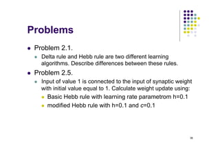
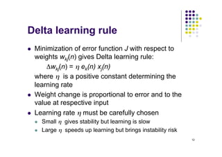
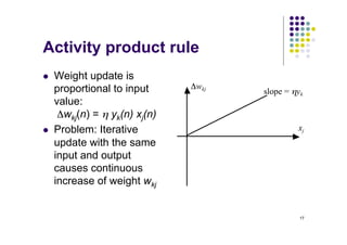
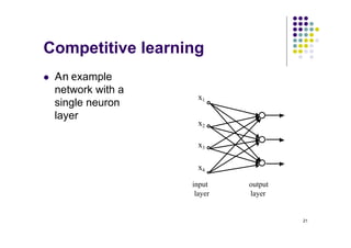
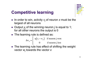
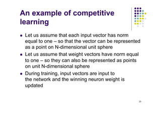
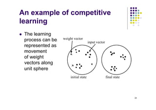
This document discusses various neural network learning processes and paradigms, including: - Error-correction learning uses a delta rule to minimize the difference between the network's output and the desired output. - Hebbian learning updates weights based on the activities of connected neurons, with rules like the activity product rule. - Competitive learning is unsupervised, with neurons competing to respond to input patterns in order to classify them. 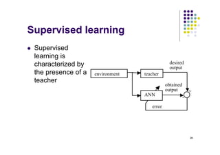- Supervised learning uses input-output pairs from a teacher to train the network, while reinforcement learning receives a grade or reward instead of examples. Unsupervised learning has no teacher.

1. 1
Neural Networks:
Learning Process
Prof. Sven Lončarić
sven.loncaric@fer.hr
http://www.fer.hr/ipg

2. 2
Overview of topics
l Introduction
l Error-correction learning
l Hebb learning
l Competitive learning
l Credit-assignment problem
l Supervised learning
l Reinforcement learning
l Unsupervised learning

3. 3
Introduction
l One of the most important ANN features is ability to
learn from the environment
l ANN learns through an iterative process of synaptic
weights and threshold adaptation
l After each iteration ANN should have more
knowledge about the environment

4. 4
Definition of learning
l Definition of learning in the ANN context:
l Learning is a process where unknown ANN parameters are
adapted through continuous process of stimulation from the
environment
l Learning is determined by the way how the change of
parameters takes place
l This definition implies the following events:
l The environment stimulates the ANN
l ANN changes due to environment
l ANN responds differently to the environment due to the
change

5. 5
Notation
l vj and vk are
activations of
neurons j and k
l xj and xk are
outputs of
neurons j and k
l Let wkj(n) be
synaptic weights
at time n
Neuron j Neuron k
ϕ(vj) ϕ(vk)
vj vk
xj xk
wkj

6. 6
Notation
l If in step n synaptic weight wkj(n) is changed
by Δwkj(n) we get the new weight:
wkj(n+1) = wkj(n) + Δwkj(n)
where wkj(n) and wkj(n+1) are old and new weights
between neurons k and j
l A set of rules that are solution to the learning
problem is called a learning algorithm
l There is no unique learning algorithm, but many
different learning algorithms, each with its
advantages and drawbacks

7. 7
Algorithms and learning
paradigms
l Learning algorithms determine how weight
correction Δwkj(n) is computed
l Learning paradigms determine the relation of the
ANN to the environment
l Three basic learning paradigms are:
l Supervised learning
l Reinforcement learning
l Unsupervised learning

8. 8
Basic learning approaches
l According to learning algorithm:
l Error-correction learning
l Hebb learning
l Competitive learning
l Boltzmann learning
l Thorndike learning
l According to learning paradigm:
• Supervised learning
• Reinforcement learning
• Unsupervised learning

9. 9
Error-correction learning
l Belongs to the supervised learning paradigm
l Let dk(n) be desired output of neuron k at moment n
l Let yk(n) be obtained output of neuron k at
moment n
l Output yk(n) is obtained using input vector x(n)
l Input vector x(n) and desired output dk(n) represent
an example that is presented to ANN at moment n
l Error is the difference between desired and obtained
output of neuron k at moment n:
ek(n) = dk(n) - yk(n)

10. 10
Error-correction learning
l The goal of error-correction learning is to minimize
an error function derived from errors ek(n) so that the
obtained output of all neurons approximates the
desired output in some statistical sense
l A frequently used error function is mean square
error:
where E[.] is the statistical expectation operator, and
summation is for all neurons in the output layer
( )⎥
⎦
⎤
⎢
⎣
⎡
= ∑
k
k n
e
E
J 2
2
1

11. 11
Error function
l The problem with minimization of error function J is
that it is necessary to know statistical properties of
random processes ek(n)
l For this reason an estimate of the error function in
step n is used as the optimization function:
l This approach yields an approximate solution
( ) ( )
∑
=
k
k n
e
n 2
2
1
E

12. 12
Delta learning rule
l Minimization of error function J with respect to
weights wkj(n) gives Delta learning rule:
Δwkj(n) = η ek(n) xj(n)
where η is a positive constant determining the
learning rate
l Weight change is proportional to error and to the
value at respective input
l Learning rate η must be carefully chosen
l Small η gives stability but learning is slow
l Large η speeds up learning but brings instability risk

13. 13
Error surface
l If we draw error value J with respect to synaptic
weights we obtain a multidimensional error surface
l The learning problem consists of finding a point on
the error surface that has the smallest error (i.e. to
minimize the error)

14. 14
Error surface
l Depending on the type of neurons there are two
possibilities:
l ANN consists of linear neurons – in this case the error
surface is a quadratic function with one global minimum
l ANN consists of nonlinear neurons – in this case the error
surface has one or more global minima and multiple local
minima
l Learning starts from an arbitrary point on the error
surface and through minimization process:
l In the first case it converges to the global minimum
l In the second case it can also converge to a local minimum

15. 15
Hebb learning
l Hebbov principle of learning says (Hebb, The
Organization of Behavior, 1942):
l When axon of neuron A is close enough to activate neuron
B and it repeats this many times there will be metabolical
changes so that efficiency of neuron A in activating neuron
B is increased
l Extension of this principle (Stent, 1973):
l If one neuron does not influence (stimulate) another neuron
then the synapse between them becomes weaker or is
completely eliminated

16. 16
Activity product rule
l According to Hebb principle weights are changed as
follows:
Δwkj(n) = F(yk(n), xj(n))
where yk(n) and xj(n) are the output and j-th input
of k-th neuron
l A special case of this prinicple is:
Δwkj(n) = η yk(n) xj(n)
where constant η determines the learning rate
l This rule is called activity product rule

17. 17
Activity product rule
l Weight update is
proportional to input
value:
Δwkj(n) = η yk(n) xj(n)
l Problem: Iterative
update with the same
input and output
causes continuous
increase of weight wkj
xj
Δwkj
slope = ηyk

18. 18
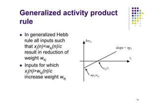
Generalized activity product
rule
l To overcome the problem of weight saturation
modifications are porposed that are aimed at limiting
the increase of weight wkj
l Non-linear limiting factor (Kohonen, 1988):
Δwkj(n) = η yk(n) xj(n) - α yk(n) wkj(n)
where α is a positive constant
l This expression can be written as:
Δwkj(n) = α yk(n)[cxj(n) - wkj(n)]
where c = η/α

19. 19
Generalized activity product
rule
l In generalized Hebb
rule all inputs such
that xj(n)<wkj(n)/c
result in reduction of
weight wkj
l Inputs for which
xj(n)>wkj(n)/c
increase weight wkj
xj
Δwkj
slope = ηyk
wkj/c
-aykwkj

20. 20
Competitive learning
l Unsupervised learning
l Neurons compete to get opportunity to become
active
l Only one neuron can be active at any time
l Useful for classification problems
l Three elements of competitive learning:
l A set of neurons having randomly selected weights, so
they have different response for a given input
l Limited weight of each neuron
l Mechanism for competition of neurons so that only one
neuron is given at any single time (winner-takes-all neuron)

21. 21
Competitive learning
l An example
network with a
single neuron
layer
input output
layer layer
x1
x2
x3
x4

22. 22
Competitive learning
l In order to win, activity vj of neuron x must be the
largest of all neurons
l Output yj of the winning neuron j is equal to 1;
for all other neurons the output is 0
l The learning rule is defined as:
l The learning rule has effect of shifting the weight
vector wj towards the vector x
Δwji =
η xi − wji
( ) if neuron j won
0 if neuron j lost
⎧
⎨
⎪
⎩
⎪

23. 23
An example of competitive
learning
l Let us assume that each input vector has norm
equal to one – so that the vector can be represented
as a point on N-dimensional unit sphere
l Let us assume that weight vectors have norm equal
to one – so they can also be represented as points
on unit N-dimensional sphere
l During training, input vectors are input to
the network and the winning neuron weight is
updated

24. 24
An example of competitive
learning
l The learning
process can be
represented as
movement
of weight
vectors along
unit sphere
initial state final state
weight vector
input vector

25. 25
Credit-assignment problem
l Credit-assignment problem is an important issue in
learning algorithms
l Credit-assignment problem is in assignment of
credit/blame for the overall learning outcome that
depends on a large number of internal decisions of
the learning system

26. 26
Supervised learning
l Supervised
learning is
characterized by
the presence of a
teacher
environment teacher
ANN
desired
output
error
obtained
output +
-

27. 27
Supervised learning
l Teacher has knowledge in the form of input-output
pairs used for training
l Error is a difference between desired and obtained
output for a given input vector
l ANN parameters change under the influence of
input vectors and error values
l The learning process is repeated until ANN learns to
imitate the teacher
l After learning is completed, the teacher is no longer
required and ANN can work without supervision

28. 28
Supervised learning
l Error function can be mean square error and it
depends on the free parameters (weights)
l Error function can be represented as a
multidimensional error surface
l Any ANN configuration is defined by weights
and corresponds to a point on the error surface
l Learning process can be viewed as movement of
the point down the error surface towards the global
minimum of the error surface

29. 29
Supervised learning
l A point on error surface moves towards the
minimum based on gradient
l The gradient at any point on the surface is a vector
showing the direction of the steepest ascent

30. 30
Supervised learning
l Examples of supervised learning algorithms are:
l LMS (least-mean-square) algorithm
l BP (back-propagation) algorithm
l A disadvantage of supervised learning is that
learning is not possible without a teacher
l ANN can only learn based on provided examples

31. 31
Supervised learning
l Suppervised learning can be implemented to work
offline or online
l In offline learning:
l ANN learns first
l When learning is completed ANN does not change any
more
l In online learning:
l ANN learns during exploitation phase
l Learning is perfomed in real-time – ANN is dynamic

32. 32
Reinforcement learning
l Reinforcement learning is of an online character
l Input-output learning mapping is learned through the
iterative process where a measure of learning
quality is maximized
l Reinforcement learning overcomes the problem of
supervised learning where training examples are
required

33. 33
Reinforcement learning
l In reinforcement learning the teacher does not
present input-output training examples, but only
gives a grade representing a measure of learning
quality
l The grade is a scalar value (a number)
l Error function is unknown in reinforcement learning
l Learning algorithm must determine direction of
motion in the learning space through a trial-and-
error approach

34. 34
Thorndike law of effect
l Reinforcement learning principle:
l If learning system actions result in positive grade then
there is higher likelihood that the system will take similar
actions in the future
l Otherwise the likelihood of taking such actions is reduced

35. 35
Unsupervised learning
l In unsupervised learning there is no teacher
assisting the learning process
l Competitive learning is an example of unsupervised
learning

36. 36
Unsupervised learning
l A layer of neurons compete for a chance to learn (to
modify their weights based on the input vector)
l In the simplest approach the winner-takes-all
strategy is used

37. 37
Comparison of supervised and
unsupervised learning
l The most popular algorithm for supervised learning
is error-backpropagation algorithm
l A disadvantage of this algorithm is bad scaling –
learning complexity grows exponentially with the
number of layers

38. 38
Problems
l Problem 2.1.
l Delta rule and Hebb rule are two different learning
algorithms. Describe differences between these rules.
l Problem 2.5.
l Input of value 1 is connected to the input of synaptic weight
with initial value equal to 1. Calculate weight update using:
l Basic Hebb rule with learning rate parametrom h=0.1
l modified Hebb rule with h=0.1 and c=0.1