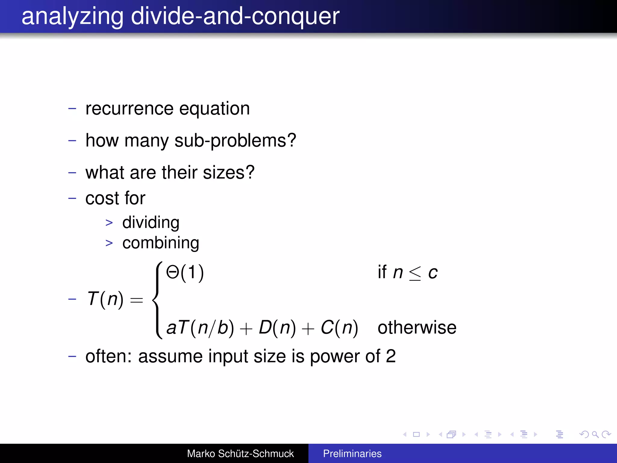
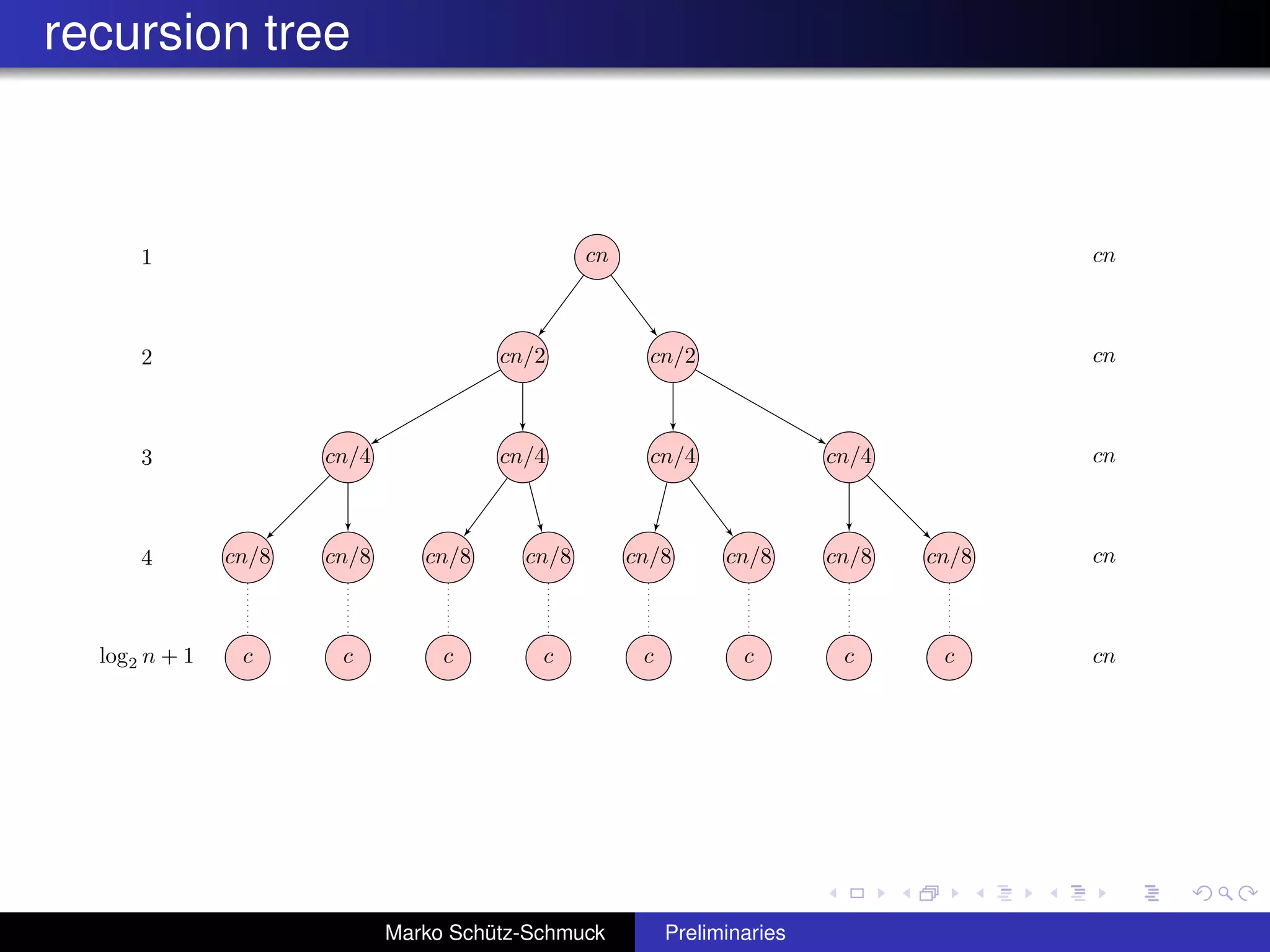
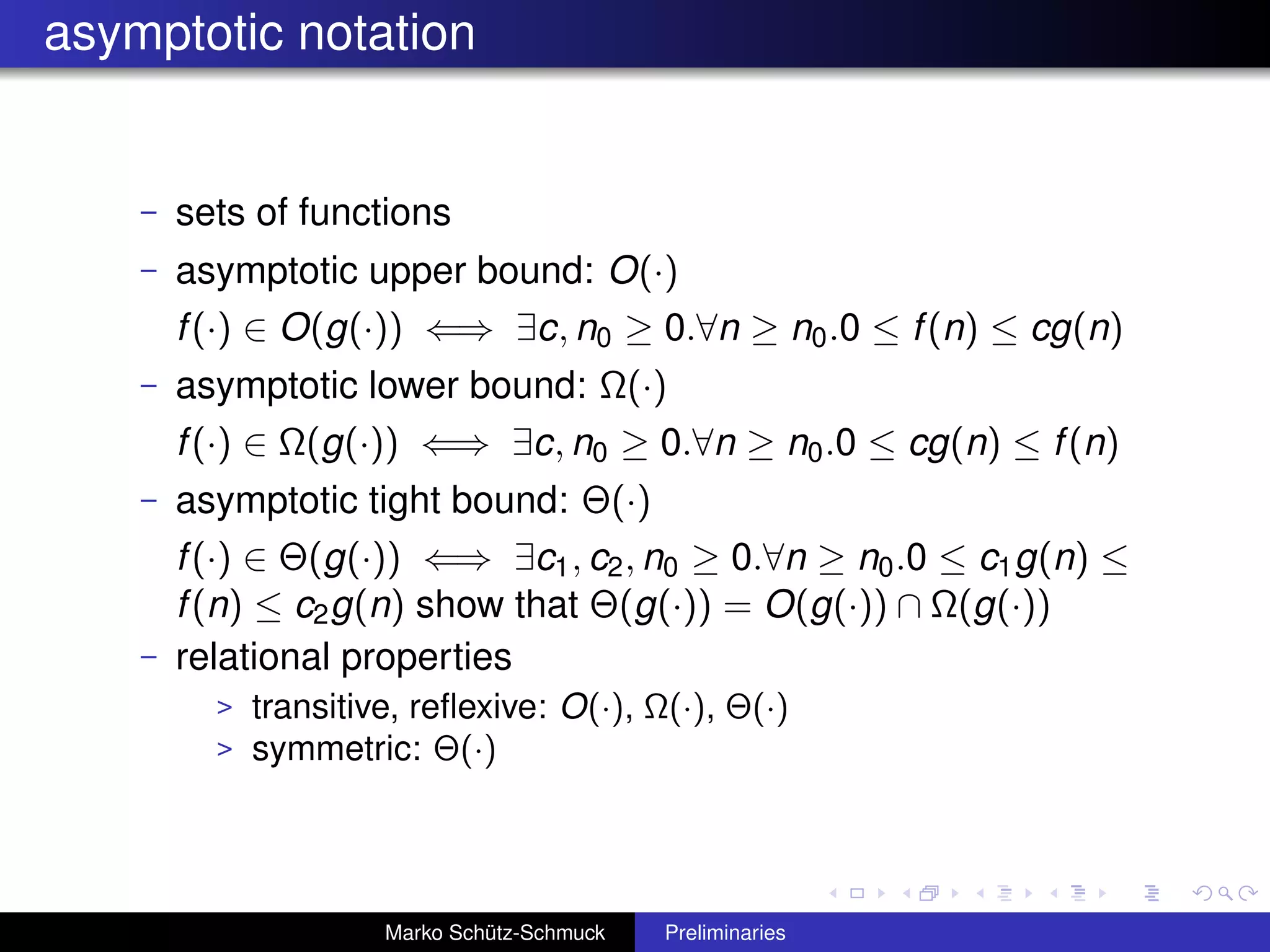
This document provides an introduction and overview of algorithm analysis and computational complexity. It discusses analyzing algorithms based on different models of computation, comparing algorithms based on efficiency measures like running time, and analyzing efficiency using asymptotic notation like Big O. Specific algorithms like insertion sort and merge sort are used as examples to illustrate concepts like best-case vs worst-case analysis and divide-and-conquer approaches.

1. Preliminaries
Marko Schütz-Schmuck
Department of Mathematical Sciences
University of Puerto Rico at Mayagüez
Mayagüez, PR
24 August 2011
Marko Schütz-Schmuck Preliminaries

2. Outline
Marko Schütz-Schmuck Preliminaries

3. Problems
– implementation/solution independent
– declarative specification
– "input/output" or "given/sought"
Marko Schütz-Schmuck Preliminaries

4. Machines
– real machines
> dedicated HW for e.g. cryptography, graphics, . . .
– abstract machines
> Turing Machine (TM)
> Random Access Machine (RAM)
> Parallel Random Access Machine (PRAM)
Marko Schütz-Schmuck Preliminaries

5. comparison of algorithms
– For given problem:
“Is algorithm A more efficient than algorithm B?”
– differences
> in machines
> in cost per instruction type
– appropriate measure?
> cost to solve specific instance
> cost depending on problem instance size
> measuring instance size?
- number of elements in the input
- number of bits in the input
Marko Schütz-Schmuck Preliminaries

6. O(·): "order of"
– theoretical justification
> time: linear speed-up theorem
> space: tape compression theorem
Marko Schütz-Schmuck Preliminaries

7. example: insertion sort
f o r j ← 2 to l e n g t h [ A ]
do key ← A [ j ]
i ← j − 1
while i > 0 and A [ i ] > key
do A [ i + 1 ] ← A [ i ]
i ← i − 1
A [ i + 1 ] ← key
– best case
here: already sorted
– worst case
here: inversely sorted
Marko Schütz-Schmuck Preliminaries

8. worst-case and average case analysis
– worst-case: upper bound for running time on any input
example: data set with frequent addition of data: search. . .
– average-case: often almost as bad as worst-case
sometimes difficult to even choose a suitable distribution
– why is best-case running time meaningless?
Marko Schütz-Schmuck Preliminaries

9. more efficient
– disregard constants
– compare only asymptotic growth
– possibly
Marko Schütz-Schmuck Preliminaries

10. algorithm design
– incremental, e.g. insertion sort
– divide-and-conquer, e.g. merge sort
Marko Schütz-Schmuck Preliminaries

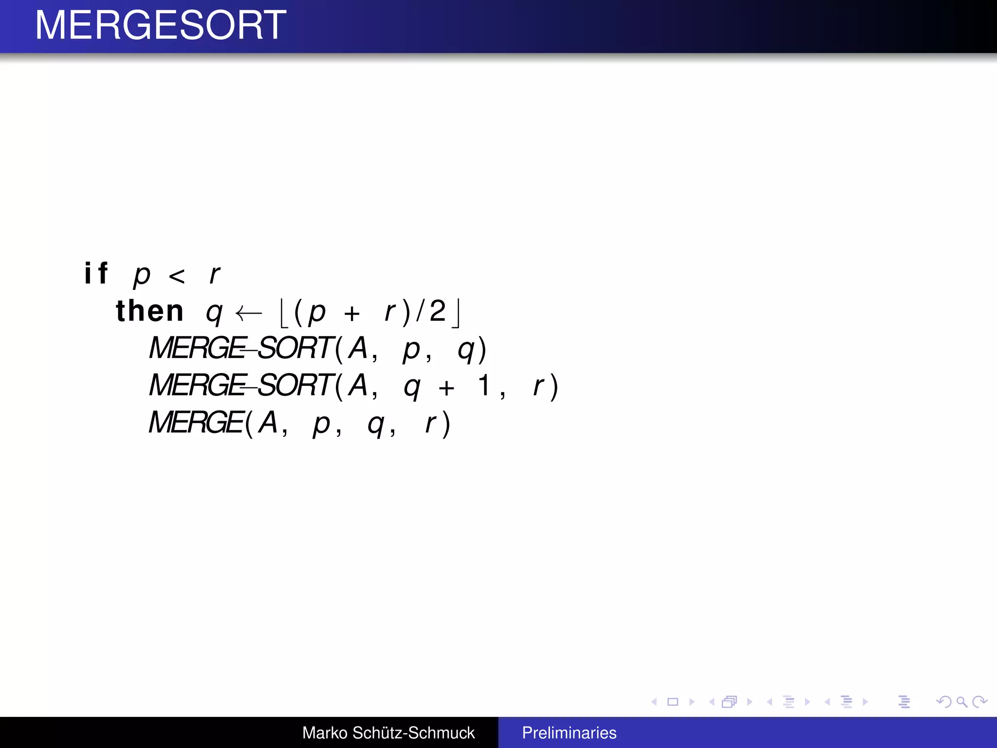
11. MERGE(A, p, q, r)
n1 ← q − p + 1
n2 ← r − q
c r e a t e a r r a y s L [ 1 . . n1 + 1 ] and R[ 1 . . n2 + 1 ]
f o r i ← 1 to n1
do L [ i ] ← A [ p + i − 1 ]
f o r j ← 1 to n2
do R[ j ] ← A [ q + j ]
L [ n1 + 1 ] ← R[ n2 + 1 ] ← ∞
i ← j ← 1
f o r k ← p to r
do i f L [ i ] ≤ R [ j ]
then A [ k ] ← L [ i ]
i ← i + 1
else A [ k ] ← R[ j ]
j ← j + 1
Marko Schütz-Schmuck Preliminaries

12. merge correctness
– assume A[p..q] and A[q + 1..r ] are each sorted
– invariant
The sub-array A[p..k − 1] contains the k − p smallest
elements of L[1..n1 + 1] and R[1..n2 + 1], in sorted order.
Moreover, L[i] and R[j] are the smallest elements of their
arrays that have not been copied back into A.
Marko Schütz-Schmuck Preliminaries

13. MERGESORT
if p < r
then q ← ( p + r ) / 2
MERGE−SORT( A , p , q )
MERGE−SORT( A , q + 1 , r )
MERGE( A , p , q , r )
Marko Schütz-Schmuck Preliminaries

14. analyzing divide-and-conquer
– recurrence equation
– how many sub-problems?
– what are their sizes?
– cost for
> dividing
> combining

Θ(1)
 if n ≤ c
– T (n) =

aT (n/b) + D(n) + C(n) otherwise

– often: assume input size is power of 2
Marko Schütz-Schmuck Preliminaries

15. recursion tree
1 cn cn
2 cn/2 cn/2 cn
3 cn/4 cn/4 cn/4 cn/4 cn
4 cn/8 cn/8 cn/8 cn/8 cn/8 cn/8 cn/8 cn/8 cn
log2 n + 1 c c c c c c c c cn
Marko Schütz-Schmuck Preliminaries

16. asymptotic notation
– sets of functions
– asymptotic upper bound: O(·)
f (·) ∈ O(g(·)) ⇐⇒ ∃c, n0 ≥ 0.∀n ≥ n0 .0 ≤ f (n) ≤ cg(n)
– asymptotic lower bound: Ω(·)
f (·) ∈ Ω(g(·)) ⇐⇒ ∃c, n0 ≥ 0.∀n ≥ n0 .0 ≤ cg(n) ≤ f (n)
– asymptotic tight bound: Θ(·)
f (·) ∈ Θ(g(·)) ⇐⇒ ∃c1 , c2 , n0 ≥ 0.∀n ≥ n0 .0 ≤ c1 g(n) ≤
f (n) ≤ c2 g(n) show that Θ(g(·)) = O(g(·)) ∩ Ω(g(·))
– relational properties
> transitive, reflexive: O(·), Ω(·), Θ(·)
> symmetric: Θ(·)
Marko Schütz-Schmuck Preliminaries