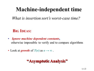
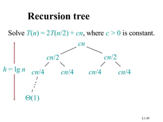
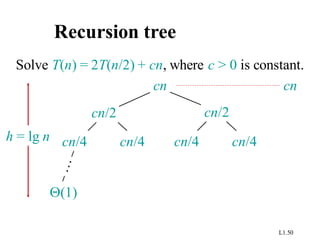
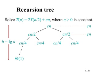
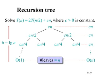
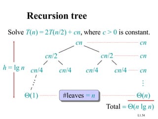
This document provides an overview of an introduction to algorithms course. It discusses insertion sort and merge sort algorithms. Insertion sort runs in O(n^2) time in the worst case, making it inefficient for large data sets. Merge sort runs in O(n log n) time, making it faster than insertion sort for most data sets. The document provides pseudocode and examples of how insertion sort and merge sort work, and uses recurrence relations and recursion trees to analyze their asymptotic runtime performances.

1. Introduction to Algorithms
6.046J
Lecture 1
Prof. Shafi Goldwasser
Prof. Erik Demaine

2. L1.2
Welcome to Introduction to
Algorithms, Spring 2004
Handouts
1. Course Information
2. Course Calendar
3. Problem Set 1
4. Akra-Bazzi Handout

3. L1.3
Course information
1. Staff
2. Prerequisites
3. Lectures & Recitations
4. Handouts
5. Textbook (CLRS)
6. Website
8. Extra Help
9. Registration
10.Problem sets
11.Describing algorithms
12.Grading policy
13.Collaboration policy

4. L1.4
What is course about?
The theoretical study of design and
analysis of computer algorithms
Basic goals for an algorithm:
• always correct
• always terminates
• This class: performance
➢ Performance often draws the line between
what is possible and what is impossible.

5. L1.5
Design and Analysis of Algorithms
• Analysis: predict the cost of an algorithm in
terms of resources and performance
• Design: design algorithms which minimize the
cost

6. L1.7
The problem of sorting
Input: sequence a1, a2, …, an of numbers.
Example:
Input: 8 2 4 9 3 6
Output: 2 3 4 6 8 9
Output: permutation a'1, a'2, …, a'n such
that a'1  a'2  …  a'n .

7. L1.8
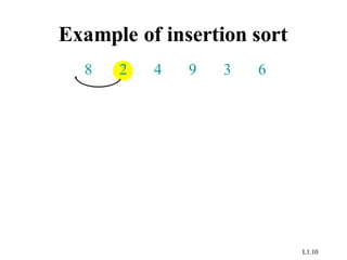
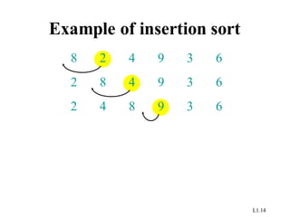
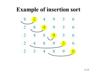
Insertion sort
INSERTION-SORT (A, n) ⊳ A[1 . . n]
for j ← 2 to n
do key ← A[ j]
i ← j – 1
while i > 0 and A[i] > key
do A[i+1] ← A[i]
i ← i – 1
A[i+1] = key
“pseudocode”
i j
key
sorted
A:
1 n

8. L1.9
Example of insertion sort
8 2 4 9 3 6

9. L1.10
Example of insertion sort
8 2 4 9 3 6

10. L1.11
Example of insertion sort
8 2 4 9 3 6
2 8 4 9 3 6

11. L1.12
Example of insertion sort
8 2 4 9 3 6
2 8 4 9 3 6

12. L1.13
Example of insertion sort
8 2 4 9 3 6
2 8 4 9 3 6
2 4 8 9 3 6

13. L1.14
Example of insertion sort
8 2 4 9 3 6
2 8 4 9 3 6
2 4 8 9 3 6

14. L1.15
Example of insertion sort
8 2 4 9 3 6
2 8 4 9 3 6
2 4 8 9 3 6
2 4 8 9 3 6

15. L1.16
Example of insertion sort
8 2 4 9 3 6
2 8 4 9 3 6
2 4 8 9 3 6
2 4 8 9 3 6

16. L1.17
Example of insertion sort
8 2 4 9 3 6
2 8 4 9 3 6
2 4 8 9 3 6
2 4 8 9 3 6
2 3 4 8 9 6

17. L1.18
Example of insertion sort
8 2 4 9 3 6
2 8 4 9 3 6
2 4 8 9 3 6
2 4 8 9 3 6
2 3 4 8 9 6

18. L1.19
Example of insertion sort
8 2 4 9 3 6
2 8 4 9 3 6
2 4 8 9 3 6
2 4 8 9 3 6
2 3 4 8 9 6
2 3 4 6 8 9 done

19. L1.20
Running time
• The running time depends on the input: an
already sorted sequence is easier to sort.
• Major Simplifying Convention:
Parameterize the running time by the size of
the input, since short sequences are easier to
sort than long ones.
➢TA(n) = time of A on length n inputs
• Generally, we seek upper bounds on the
running time, to have a guarantee of
performance.

20. L1.21
Kinds of analyses
Worst-case: (usually)
• T(n) = maximum time of algorithm
on any input of size n.
Average-case: (sometimes)
• T(n) = expected time of algorithm
over all inputs of size n.
• Need assumption of statistical
distribution of inputs.
Best-case: (NEVER)
• Cheat with a slow algorithm that
works fast on some input.

21. L1.22
Machine-independent time
What is insertion sort’s worst-case time?
BIG IDEAS:
• Ignore machine dependent constants,
otherwise impossible to verify and to compare algorithms
• Look at growth of T(n) as n → ∞ .
“AsymptoticAnalysis”

22. L1.23
Q-notation
• Drop low-order terms; ignore leading constants.
• Example: 3n3 + 90n2 – 5n + 6046 = Q(n3)
DEF:
Q(g(n)) = { f (n) : there exist positive constants c1, c2, and
n0 such that 0  c1 g(n)  f (n)  c2 g(n)
for all n  n0 }
Basic manipulations:

23. L1.24
Asymptotic performance
n
T(n)
n0
.
• Asymptotic analysis is a
useful tool to help to
structure our thinking
toward better algorithm
• We shouldn’t ignore
asymptotically slower
algorithms, however.
• Real-world design
situations often call for a
careful balancing
When n gets large enough, a Q(n2) algorithm
always beats a Q(n3) algorithm.

24. L1.25
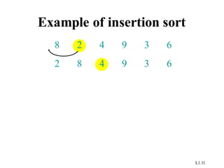
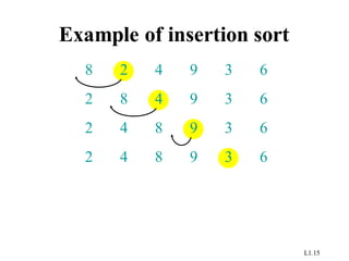
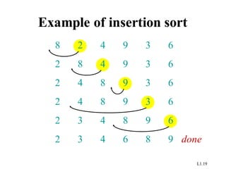
Insertion sort analysis
Worst case: Input reverse sorted.
( )

=
Q
=
Q
=
n
j
n
j
n
T
2
2
)
(
)
(
Average case: All permutations equally likely.
( )

=
Q
=
Q
=
n
j
n
j
n
T
2
2
)
2
/
(
)
(
Is insertion sort a fast sorting algorithm?
• Moderately so, for small n.
• Not at all, for large n.
[arithmetic series]

25. L1.26
Example 2: Integer
Multiplication
• Let X = A B and Y = C D where A,B,C
and D are n/2 bit integers
• Simple Method: XY = (2n/2A+B)(2n/2C+D)
• Running Time Recurrence
T(n) < 4T(n/2) + 100n
• Solution T(n) = q(n2)

26. L1.27
Better Integer Multiplication
• Let X = A B and Y = C D where A,B,C and D
are n/2 bit integers
• Karatsuba:
XY = (2n/2+2n)AC+2n/2(A-B)(C-D) + (2n/2+1) BD
• Running Time Recurrence
T(n) < 3T(n/2) + 100n
• Solution: q(n) = O(n log 3)

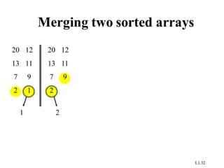
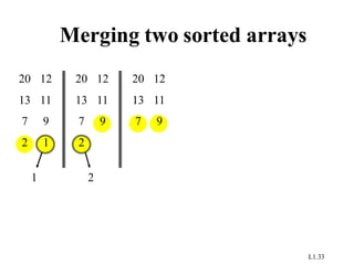
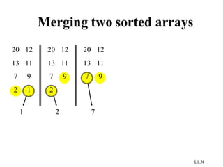
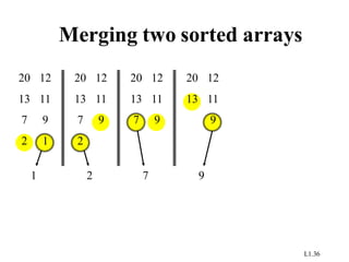
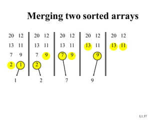
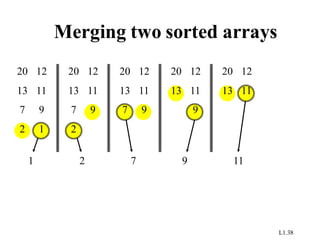
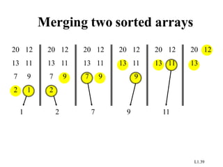
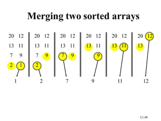
27. L1.28
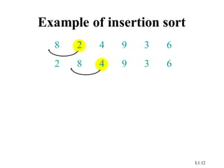
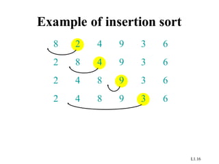
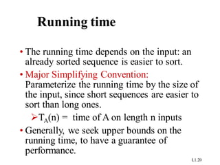
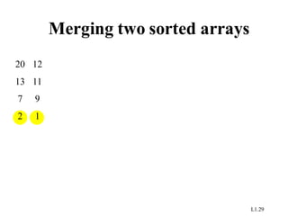
Example 3:Merge sort
MERGE-SORT A[1 . . n]
1. If n = 1, done.
2. Recursively sort A[ 1 . . n/2 ]
and A[ n/2+1 . . n ] .
3. “Merge” the 2 sorted lists.
Key subroutine: MERGE

28. L1.29
Merging two sorted arrays
20
13
7
2
12
11
9
1

29. L1.30
Merging two sorted arrays
20
13
7
2
12
11
9
1
1

30. L1.31
Merging two sorted arrays
20
13
7
2
12
11
9
1
1
20
13
7
2
12
11
9

31. L1.32
Merging two sorted arrays
20
13
7
2
12
11
9
1
1
20
13
7
2
12
11
9
2

32. L1.33
Merging two sorted arrays
20
13
7
2
12
11
9
1
1
20
13
7
2
12
11
9
2
20
13
7
12
11
9

33. L1.34
Merging two sorted arrays
20
13
7
2
12
11
9
1
1
20
13
7
2
12
11
9
2
20
13
7
12
11
9
7

34. L1.35
Merging two sorted arrays
20
13
7
2
12
11
9
1
1
20
13
7
2
12
11
9
2
20
13
7
12
11
9
7
20
13
12
11
9

35. L1.36
Merging two sorted arrays
20
13
7
2
12
11
9
1
1
20
13
7
2
12
11
9
2
20
13
7
12
11
9
7
20
13
12
11
9
9

36. L1.37
Merging two sorted arrays
20
13
7
2
12
11
9
1
1
20
13
7
2
12
11
9
2
20
13
7
12
11
9
7
20
13
12
11
9
9
20
13
12
11

37. L1.38
Merging two sorted arrays
20
13
7
2
12
11
9
1
1
20
13
7
2
12
11
9
2
20
13
7
12
11
9
7
20
13
12
11
9
9
20
13
12
11
11

38. L1.39
Merging two sorted arrays
20
13
7
2
12
11
9
1
1
20
13
7
2
12
11
9
2
20
13
7
12
11
9
7
20
13
12
11
9
9
20
13
12
11
11
20
13
12

39. L1.40
Merging two sorted arrays
20
13
7
2
12
11
9
1
1
20
13
7
2
12
11
9
2
20
13
7
12
11
9
7
20
13
12
11
9
9
20
13
12
11
11
20
13
12
12

40. L1.41
Merging two sorted arrays
20
13
7
2
12
11
9
1
1
20
13
7
2
12
11
9
2
20
13
7
12
11
9
7
20
13
12
11
9
9
20
13
12
11
11
20
13
12
12
Time = Q(n) to merge a total
of n elements (linear time).

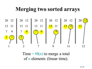
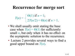
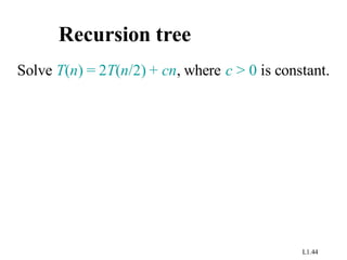
41. L1.42
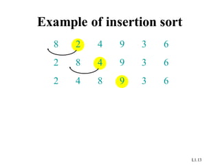
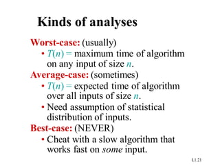
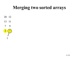
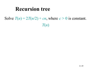
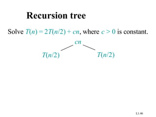
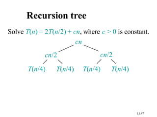
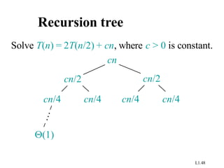
Analyzing merge sort
MERGE-SORT A[1 . . n]
1. If n = 1, done.
2. Recursively sort A[ 1 . . n/2 ]
and A[ n/2+1 . . n ] .
3. “Merge” the 2 sorted lists
T(n)
Q(1)
2T(n/2)
Q(n)
Sloppiness: Should be T( n/2 ) + T( n/2 ) ,
but it turns out not to matter asymptotically.

42. L1.43
Recurrence for merge sort
T(n) =
Q(1) if n = 1;
2T(n/2) + Q(n) if n > 1.
• We shall usually omit stating the base
case when T(n) = Q(1) for sufficiently
small n, but only when it has no effect on
the asymptotic solution to the recurrence.
• Lecture 2 provides several ways to find a
good upper bound on T(n).

43. L1.44
Recursion tree
Solve T(n) = 2T(n/2) + cn, where c > 0 is constant.

44. L1.45
Recursion tree
Solve T(n) = 2T(n/2) + cn, where c > 0 is constant.
T(n)

45. L1.46
Recursion tree
Solve T(n) = 2T(n/2) + cn, where c > 0 is constant.
T(n/2) T(n/2)
cn

46. L1.47
Recursion tree
Solve T(n) = 2T(n/2) + cn, where c > 0 is constant.
cn
T(n/4) T(n/4) T(n/4) T(n/4)
cn/2 cn/2

47. L1.48
Recursion tree
Solve T(n) = 2T(n/2) + cn, where c > 0 is constant.
cn
cn/4 cn/4 cn/4 cn/4
cn/2 cn/2
Q(1)

48. L1.49
Recursion tree
Solve T(n) = 2T(n/2) + cn, where c > 0 is constant.
cn
cn/4 cn/4 cn/4 cn/4
cn/2 cn/2
Q(1)
h = lg n

49. L1.50
Recursion tree
Solve T(n) = 2T(n/2) + cn, where c > 0 is constant.
cn
cn/4 cn/4 cn/4 cn/4
cn/2 cn/2
Q(1)
h = lg n
cn

50. L1.51
Recursion tree
Solve T(n) = 2T(n/2) + cn, where c > 0 is constant.
cn
cn/4 cn/4 cn/4 cn/4
cn/2 cn/2
Q(1)
h = lg n
cn
cn

51. L1.52
Recursion tree
Solve T(n) = 2T(n/2) + cn, where c > 0 is constant.
cn
cn/4 cn/4 cn/4 cn/4
cn/2 cn/2
Q(1)
h = lg n
cn
cn
cn
…

52. L1.53
Recursion tree
Solve T(n) = 2T(n/2) + cn, where c > 0 is constant.
cn
cn/4 cn/4 cn/4 cn/4
cn/2 cn/2
Q(1)
h = lg n
cn
cn
cn
#leaves = n Q(n)
…

53. L1.54
Recursion tree
Solve T(n) = 2T(n/2) + cn, where c > 0 is constant.
cn
cn/4 cn/4 cn/4 cn/4
cn/2 cn/2
Q(1)
h = lg n
cn
cn
cn
#leaves = n Q(n)
Total = Q(n lg n)
…

54. L1.55
Conclusions
• Q(n lg n) grows more slowly than Q(n2).
• Therefore, merge sort asymptotically
beats insertion sort in the worst case.
• In practice, merge sort beats insertion
sort for n > 30 or so.