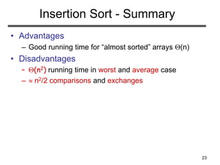
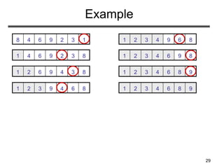
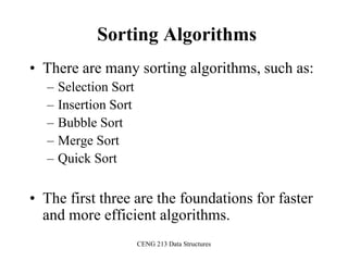
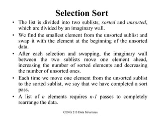
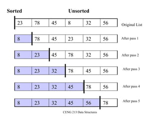
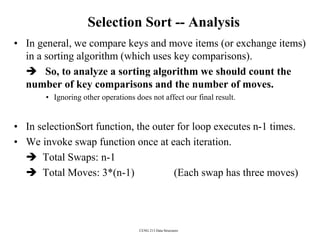
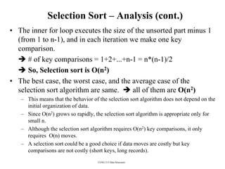
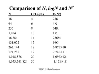
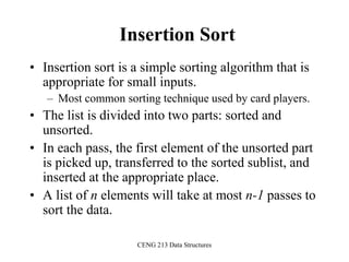
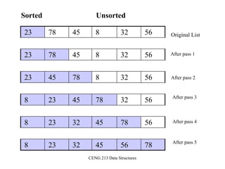
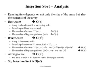
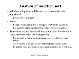
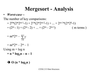
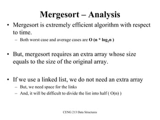
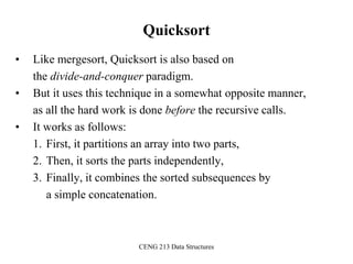
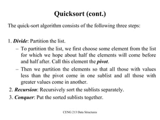
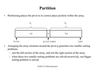
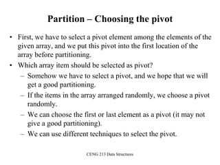
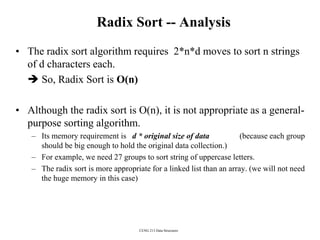
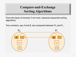
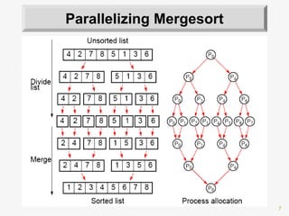
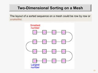
The document discusses sorting algorithms. It begins by defining the sorting problem as taking an unsorted sequence of numbers and outputting a permutation of the numbers in ascending order. It then discusses different types of sorts like internal versus external sorts and stable versus unstable sorts. Specific algorithms covered include insertion sort, bubble sort, and selection sort. Analysis is provided on the best, average, and worst case time complexity of insertion sort.

![13
INSERTION-SORT
Alg.: INSERTION-SORT(A)
for j ← 2 to n
do key ← A[ j ]
Insert A[ j ] into the sorted sequence A[1 . . j -1]
i ← j - 1
while i > 0 and A[i] > key
do A[i + 1] ← A[i]
i ← i – 1
A[i + 1] ← key
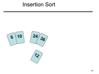
• Insertion sort – sorts the elements in place
a8a7a6a5a4a3a2a1
1 2 3 4 5 6 7 8
key](https://image.slidesharecdn.com/sorting-151213045143/85/Sorting-13-320.jpg)
![14
Loop Invariant for Insertion Sort
Alg.: INSERTION-SORT(A)
for j ← 2 to n
do key ← A[ j ]
Insert A[ j ] into the sorted sequence A[1 . . j -1]
i ← j - 1
while i > 0 and A[i] > key
do A[i + 1] ← A[i]
i ← i – 1
A[i + 1] ← key
Invariant: at the start of the for loop the elements in A[1 . . j-1]
are in sorted order](https://image.slidesharecdn.com/sorting-151213045143/85/Sorting-14-320.jpg)
![16
Loop Invariant for Insertion Sort
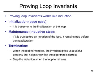
• Initialization:
– Just before the first iteration, j = 2:
the subarray A[1 . . j-1] = A[1],
(the element originally in A[1]) – is
sorted](https://image.slidesharecdn.com/sorting-151213045143/85/Sorting-16-320.jpg)
![17
Loop Invariant for Insertion Sort
• Maintenance:
– the while inner loop moves A[j -1], A[j -2], A[j -3],
and so on, by one position to the right until the proper
position for key (which has the value that started out in
A[j]) is found
– At that point, the value of key is placed into this
position.](https://image.slidesharecdn.com/sorting-151213045143/85/Sorting-17-320.jpg)
![18
Loop Invariant for Insertion Sort
• Termination:
– The outer for loop ends when j = n + 1 j-1 = n
– Replace n with j-1 in the loop invariant:
• the subarray A[1 . . n] consists of the elements originally in
A[1 . . n], but in sorted order
• The entire array is sorted!
jj - 1
Invariant: at the start of the for loop the elements in A[1 . . j-1]
are in sorted order](https://image.slidesharecdn.com/sorting-151213045143/85/Sorting-18-320.jpg)
![19
Analysis of Insertion Sort
cost times
c1 n
c2 n-1
0 n-1
c4 n-1
c5
c6
c7
c8 n-1
n
j jt2
n
j jt2
)1(
n
j jt2
)1(
)1(11)1()1()( 8
2
7
2
6
2
5421
nctctctcncncncnT
n
j
j
n
j
j
n
j
j
INSERTION-SORT(A)
for j ← 2 to n
do key ← A[ j ]
Insert A[ j ] into the sorted sequence A[1 . . j -1]
i ← j - 1
while i > 0 and A[i] > key
do A[i + 1] ← A[i]
i ← i – 1
A[i + 1] ← key
tj: # of times the while statement is executed at iteration j](https://image.slidesharecdn.com/sorting-151213045143/85/Sorting-19-320.jpg)
![20
Best Case Analysis
• The array is already sorted
– A[i] ≤ key upon the first time the while loop test is run
(when i = j -1)
– tj = 1
• T(n) = c1n + c2(n -1) + c4(n -1) + c5(n -1) + c8(n-1)
= (c1 + c2 + c4 + c5 + c8)n + (c2 + c4 + c5 + c8)
= an + b = (n)
“while i > 0 and A[i] > key”
)1(11)1()1()( 8
2
7
2
6
2
5421
nctctctcncncncnT
n
j
j
n
j
j
n
j
j](https://image.slidesharecdn.com/sorting-151213045143/85/Sorting-20-320.jpg)
![21
Worst Case Analysis
• The array is in reverse sorted order
– Always A[i] > key in while loop test
– Have to compare key with all elements to the left of the j-th
position compare with j-1 elements tj = j
a quadratic function of n
• T(n) = (n2) order of growth in n2
1 2 2
( 1) ( 1) ( 1)
1 ( 1)
2 2 2
n n n
j j j
n n n n n n
j j j
)1(
2
)1(
2
)1(
1
2
)1(
)1()1()( 8765421
nc
nn
c
nn
c
nn
cncncncnT
cbnan 2
“while i > 0 and A[i] > key”
)1(11)1()1()( 8
2
7
2
6
2
5421
nctctctcncncncnT
n
j
j
n
j
j
n
j
j
using we have:](https://image.slidesharecdn.com/sorting-151213045143/85/Sorting-21-320.jpg)
![22
Comparisons and Exchanges in
Insertion Sort
INSERTION-SORT(A)
for j ← 2 to n
do key ← A[ j ]
Insert A[ j ] into the sorted sequence A[1 . . j -1]
i ← j - 1
while i > 0 and A[i] > key
do A[i + 1] ← A[i]
i ← i – 1
A[i + 1] ← key
cost times
c1 n
c2 n-1
0 n-1
c4 n-1
c5
c6
c7
c8 n-1
n
j jt2
n
j jt2
)1(
n
j jt2
)1(
n2/2 comparisons
n2/2 exchanges](https://image.slidesharecdn.com/sorting-151213045143/85/Sorting-22-320.jpg)
![26
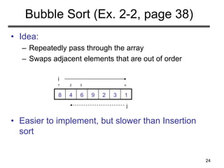
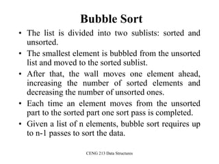
Bubble Sort
Alg.: BUBBLESORT(A)
for i 1 to length[A]
do for j length[A] downto i + 1
do if A[j] < A[j -1]
then exchange A[j] A[j-1]
1329648
i = 1 j
i](https://image.slidesharecdn.com/sorting-151213045143/85/Sorting-26-320.jpg)
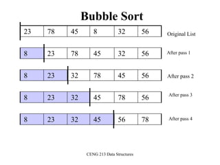
![27
Bubble-Sort Running Time
Thus,T(n) = (n2)
2
2
1 1 1
( 1)
( )
2 2 2
n n n
i i i
n n n n
where n i n i n
Alg.: BUBBLESORT(A)
for i 1 to length[A]
do for j length[A] downto i + 1
do if A[j] < A[j -1]
then exchange A[j] A[j-1]
T(n) = c1(n+1) +
n
i
in
1
)1(c2 c3
n
i
in
1
)( c4
n
i
in
1
)(
= (n) + (c2 + c2 + c4)
n
i
in
1
)(
Comparisons: n2/2
Exchanges: n2/2
c1
c2
c3
c4](https://image.slidesharecdn.com/sorting-151213045143/85/Sorting-27-320.jpg)
![30
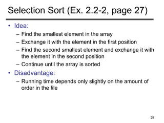
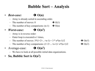
Selection Sort
Alg.: SELECTION-SORT(A)
n ← length[A]
for j ← 1 to n - 1
do smallest ← j
for i ← j + 1 to n
do if A[i] < A[smallest]
then smallest ← i
exchange A[j] ↔ A[smallest]
1329648](https://image.slidesharecdn.com/sorting-151213045143/85/Sorting-30-320.jpg)
![31
n2/2
comparisons
Analysis of Selection Sort
Alg.: SELECTION-SORT(A)
n ← length[A]
for j ← 1 to n - 1
do smallest ← j
for i ← j + 1 to n
do if A[i] < A[smallest]
then smallest ← i
exchange A[j] ↔ A[smallest]
cost times
c1 1
c2 n
c3 n-1
c4
c5
c6
c7 n-1
1
1
)1(
n
j
jn
1
1
)(
n
j
jn
1
1
)(
n
j
jn
n
exchanges
1 1 1
2
1 2 3 4 5 6 7
1 1 2
( ) ( 1) ( 1) ( 1) ( )
n n n
j j j
T n c c n c n c n j c n j c n j c n n
](https://image.slidesharecdn.com/sorting-151213045143/85/Sorting-31-320.jpg)
![CENG 213 Data Structures
Selection Sort (cont.)
template <class Item>
void selectionSort( Item a[], int n) {
for (int i = 0; i < n-1; i++) {
int min = i;
for (int j = i+1; j < n; j++)
if (a[j] < a[min]) min = j;
swap(a[i], a[min]);
}
}
template < class Object>
void swap( Object &lhs, Object &rhs )
{
Object tmp = lhs;
lhs = rhs;
rhs = tmp;
}](https://image.slidesharecdn.com/sorting-151213045143/85/Sorting-37-320.jpg)
![CENG 213 Data Structures
Insertion Sort Algorithm
template <class Item>
void insertionSort(Item a[], int n)
{
for (int i = 1; i < n; i++)
{
Item tmp = a[i];
for (int j=i; j>0 && tmp < a[j-1]; j--)
a[j] = a[j-1];
a[j] = tmp;
}
}](https://image.slidesharecdn.com/sorting-151213045143/85/Sorting-43-320.jpg)
![CENG 213 Data Structures
Bubble Sort Algorithm
template <class Item>
void bubleSort(Item a[], int n)
{
bool sorted = false;
int last = n-1;
for (int i = 0; (i < last) && !sorted; i++){
sorted = true;
for (int j=last; j > i; j--)
if (a[j-1] > a[j]{
swap(a[j],a[j-1]);
sorted = false; // signal exchange
}
}
}](https://image.slidesharecdn.com/sorting-151213045143/85/Sorting-48-320.jpg)
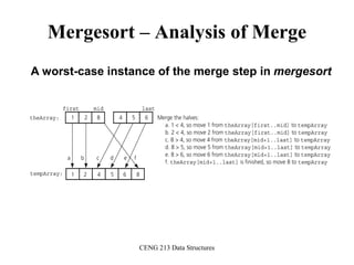
![CENG 213 Data Structures
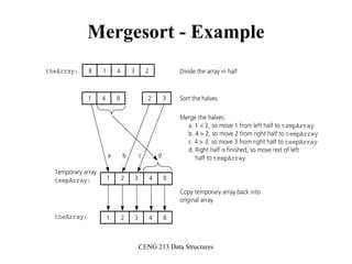
Merge
const int MAX_SIZE = maximum-number-of-items-in-array;
void merge(DataType theArray[], int first, int mid, int last)
{
DataType tempArray[MAX_SIZE]; // temporary array
int first1 = first; // beginning of first subarray
int last1 = mid; // end of first subarray
int first2 = mid + 1; // beginning of second subarray
int last2 = last; // end of second subarray
int index = first1; // next available location in tempArray
for ( ; (first1 <= last1) && (first2 <= last2); ++index) {
if (theArray[first1] < theArray[first2]) {
tempArray[index] = theArray[first1];
++first1;
}
else {
tempArray[index] = theArray[first2];
++first2;
} }](https://image.slidesharecdn.com/sorting-151213045143/85/Sorting-52-320.jpg)
![CENG 213 Data Structures
Merge (cont.)
// finish off the first subarray, if necessary
for (; first1 <= last1; ++first1, ++index)
tempArray[index] = theArray[first1];
// finish off the second subarray, if necessary
for (; first2 <= last2; ++first2, ++index)
tempArray[index] = theArray[first2];
// copy the result back into the original array
for (index = first; index <= last; ++index)
theArray[index] = tempArray[index];
} // end merge](https://image.slidesharecdn.com/sorting-151213045143/85/Sorting-53-320.jpg)
![CENG 213 Data Structures
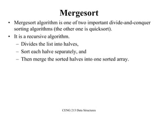
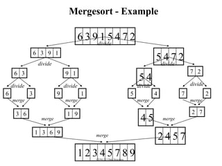
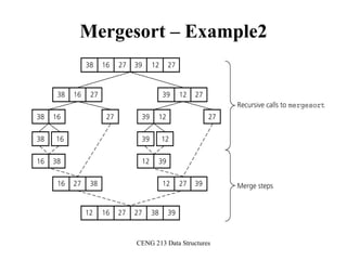
Mergesort
void mergesort(DataType theArray[], int first, int last) {
if (first < last) {
int mid = (first + last)/2; // index of midpoint
mergesort(theArray, first, mid);
mergesort(theArray, mid+1, last);
// merge the two halves
merge(theArray, first, mid, last);
}
} // end mergesort](https://image.slidesharecdn.com/sorting-151213045143/85/Sorting-54-320.jpg)
![CENG 213 Data Structures
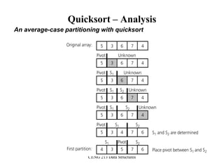
Partition Function
template <class DataType>
void partition(DataType theArray[], int first, int last,
int &pivotIndex) {
// Partitions an array for quicksort.
// Precondition: first <= last.
// Postcondition: Partitions theArray[first..last] such that:
// S1 = theArray[first..pivotIndex-1] < pivot
// theArray[pivotIndex] == pivot
// S2 = theArray[pivotIndex+1..last] >= pivot
// Calls: choosePivot and swap.
// place pivot in theArray[first]
choosePivot(theArray, first, last);
DataType pivot = theArray[first]; // copy pivot](https://image.slidesharecdn.com/sorting-151213045143/85/Sorting-67-320.jpg)
![CENG 213 Data Structures
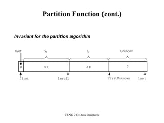
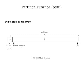
Partition Function (cont.)
// initially, everything but pivot is in unknown
int lastS1 = first; // index of last item in S1
int firstUnknown = first + 1; //index of 1st item in unknown
// move one item at a time until unknown region is empty
for (; firstUnknown <= last; ++firstUnknown) {
// Invariant: theArray[first+1..lastS1] < pivot
// theArray[lastS1+1..firstUnknown-1] >= pivot
// move item from unknown to proper region
if (theArray[firstUnknown] < pivot) { // belongs to S1
++lastS1;
swap(theArray[firstUnknown], theArray[lastS1]);
} // else belongs to S2
}
// place pivot in proper position and mark its location
swap(theArray[first], theArray[lastS1]);
pivotIndex = lastS1;
} // end partition](https://image.slidesharecdn.com/sorting-151213045143/85/Sorting-68-320.jpg)
![CENG 213 Data Structures
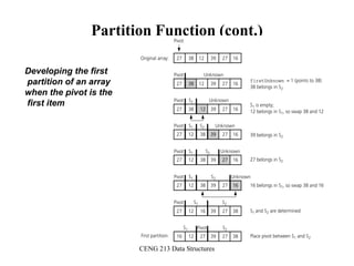
Partition Function (cont.)
Moving theArray[firstUnknown] into S1 by swapping it with
theArray[lastS1+1] and by incrementing both lastS1 and firstUnknown.](https://image.slidesharecdn.com/sorting-151213045143/85/Sorting-71-320.jpg)
![CENG 213 Data Structures
Partition Function (cont.)
Moving theArray[firstUnknown] into S2 by incrementing firstUnknown.](https://image.slidesharecdn.com/sorting-151213045143/85/Sorting-72-320.jpg)
![CENG 213 Data Structures
Quicksort Function
void quicksort(DataType theArray[], int first, int last) {
// Sorts the items in an array into ascending order.
// Precondition: theArray[first..last] is an array.
// Postcondition: theArray[first..last] is sorted.
// Calls: partition.
int pivotIndex;
if (first < last) {
// create the partition: S1, pivot, S2
partition(theArray, first, last, pivotIndex);
// sort regions S1 and S2
quicksort(theArray, first, pivotIndex-1);
quicksort(theArray, pivotIndex+1, last);
}
}](https://image.slidesharecdn.com/sorting-151213045143/85/Sorting-74-320.jpg)
![CENG 213 Data Structures
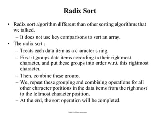
Radix Sort - Algorithm
radixSort(inout theArray:ItemArray, in n:integer, in d:integer)
// sort n d-digit integers in the array theArray
for (j=d down to 1) {
Initialize 10 groups to empty
Initialize a counter for each group to 0
for (i=0 through n-1) {
k = jth digit of theArray[i]
Place theArrar[i] at the end of group k
Increase kth counter by 1
}
Replace the items in theArray with all the items in group 0,
followed by all the items in group 1, and so on.
}](https://image.slidesharecdn.com/sorting-151213045143/85/Sorting-82-320.jpg)
![26
Number of elements that are smaller than each selected element is
counted. This count provides the position of the selected number, its
“rank” in the sorted list.
• First a[0] is read and compared with each of the other numbers,
a[1] … a[n-1], recording the number of elements less than a[0].
Suppose this number is x. This is the index of a[0] in the final
sorted list.
• The number a[0] is copied into the final sorted list b[0] … b[n-1],
at location b[x]. Actions repeated with the other numbers.
Overall sequential time complexity of rank sort: Tseq = O(n2)
(not a good sequential sorting algorithm!)
Rank Sort](https://image.slidesharecdn.com/sorting-151213045143/85/Sorting-110-320.jpg)
![27
for (i = 0; i < n; i++) { /* for each number */
x = 0;
for (j = 0; j < n; j++) /* count number less than it */
if (a[i] > a[j]) x++;
b[x] = a[i]; /* copy number into correct place */
}
*This code needs to be fixed if duplicates exist in the sequence.
Sequential code
sequential time complexity of rank sort: Tseq = O(n2)](https://image.slidesharecdn.com/sorting-151213045143/85/Sorting-111-320.jpg)
![28
One number is assigned to each processor.
Pi finds the final index of a[i] in O(n) steps.
forall (i = 0; i < n; i++) { /* for each no. in parallel*/
x = 0;
for (j = 0; j < n; j++) /* count number less than it */
if (a[i] > a[j]) x++;
b[x] = a[i]; /* copy no. into correct place */
}
Parallel time complexity, O(n), as good as any sorting algorithm so
far. Can do even better if we have more processors.
Parallel Rank Sort (P=n)
Parallel time complexity: Tpar = O(n) (for P=n)](https://image.slidesharecdn.com/sorting-151213045143/85/Sorting-112-320.jpg)
![29
Use n processors to find the rank of one element. The final count,
i.e. rank of a[i] can be obtained using a binary addition operation
(global sum MPI_Reduce())
Parallel Rank Sort with P = n2
Time complexity
(for P=n2):
Tpar = O(log n)
Can we do it in O(1) ?](https://image.slidesharecdn.com/sorting-151213045143/85/Sorting-113-320.jpg)