The document describes insertion sort, a sorting algorithm. Insertion sort iterates through an unsorted array and inserts each element into its sorted position. This has a worst-case running time of O(n^2) because in each iteration, elements may need to be shifted to make space for the new element. The document also introduces asymptotic notation for analyzing algorithm running times, such as O(), Ω(), and Θ().

1. Lecture given at the International Summer School Modern Computational Science
(August 15-26, 2011, Oldenburg, Germany)
Basic Introduction into Algorithms and Data
Structures
Frauke Liers
Computer Science Department
University of Cologne
D-50969 Cologne
Germany
Abstract. This chapter gives a brief introduction into basic data structures and
algorithms, together with references to tutorials available in the literature. We first
introduce fundamental notation and algorithmic concepts. We then explain several
sorting algorithms and give small examples. As fundamental data structures, we in-
troduce linked lists, trees and graphs. Implementations are given in the programming
language C.
Contents
1 Introduction . . . . . . . . . . . . . . . . . . . . . . . . . . . 2
2 Sorting . . . . . . . . . . . . . . . . . . . . . . . . . . . . . . 2
2.1 Insertion Sort . . . . . . . . . . . . . . . . . . . . . . . . . . 3
2.1.1 Some Basic Notation and Analysis of Insertion Sort . . . 4
2.2 Sorting using the Divide-and-Conquer Principle . . . . . . . 7
2.2.1 Merge Sort . . . . . . . . . . . . . . . . . . . . . . . . . . 7
2.2.2 Quicksort . . . . . . . . . . . . . . . . . . . . . . . . . . . 9
2.3 A Lower Bound on the Performance of Sorting Algorithms 12
3 Select the k-th smallest element . . . . . . . . . . . . . . . 12
4 Binary Search . . . . . . . . . . . . . . . . . . . . . . . . . . 13
5 Elementary Data Structures . . . . . . . . . . . . . . . . . 14
5.1 Stacks . . . . . . . . . . . . . . . . . . . . . . . . . . . . . . 15
1

2. Algorithms and Data Structures (Liers)
5.2 Linked Lists . . . . . . . . . . . . . . . . . . . . . . . . . . . 17
5.3 Graphs, Trees, and Binary Search Trees . . . . . . . . . . . 18
6 Advanced Programming . . . . . . . . . . . . . . . . . . . . 21
6.1 References . . . . . . . . . . . . . . . . . . . . . . . . . . . . 21
1 Introduction
This chapter is meant as a basic introduction into elementary algorithmic principles
and data structures used in computer science. In the latter field, the focus is on
processing information in a systematic and often automatized way. One goal in the
design of solution methods (algorithms) is about making efficient use of hardware
resources such as computing time and memory. It is true that hardware develop-
ment is very fast; the processors’ speed increases rapidly. Furthermore, memory has
become cheap. One could therefore ask why it is still necessary to study how these
resources can be used efficiently. The answer is simple: Despite this rapid develop-
ment, computer speed and memory are still limited. Due to the fact that the increase
in available data is even more rapid than the hardware development and for some
complex applications, we need to make efficient use of the resources.
In this introductory chapter about algorithms and data structures, we cannot cover
more than some elementary principles of algorithms and some of the relevant data
structures. This chapter cannot replace a self-study of one of the famous textbooks
that are especially written as tutorials for beginners in this field. Many very well-
written tutorials exist. Here, we only want to mention a few of them specifically.
The excellent book ‘Introduction to Algorithms’ [5] covers in detail the foundations
of algorithms and data structures. One should also look into the famous textbook
‘The art of computer programming, Volume 3: Sorting and Searching’[7] written by
Donald Knuth and into ‘Algorithms in C’[8]. We warmly recommend these and other
textbooks to the reader.
First, of course, we need to explain what an algorithm is. Loosely and not very
formally speaking, an algorithm is a method that performs a finite list of instructions
that are well-defined. A program is a specific formulation of an abstract algorithm.
Usually, it is written in a programming language and uses certain data structures.
Usually, it takes a certain specification of the problem as input and runs an algorithm
for determining a solution.
2 Sorting
Sorting is a fundamental task that needs to be performed as subroutine in many
computer programs. Sorting also serves as an introductory problem that computer
science students usually study in their first year. As input, we are given a sequence
of n natural numbers a1, a2, . . . , an that are not necessarily all pairwise different.
As an output, we want to receive a permutation (reordering) a′
1, a′
2, . . . , a′
n of the
2

3. 2 Sorting
numbers such that a′
1 ≤ a′
2 ≤ . . . ≤ a′
n. In principle, there are n! many permutations
of n elements. Of course, this number grows quickly already for small values of n such
that we need effective methods that can quickly determine a sorted sequence. Some
methods will be introduced in the following. In general, all input that is necessary for
the method to determine a solution is called an instance. In our case, it is a specific
series of numbers that needs to be sorted. For example, suppose we want to sort
the instance 9, 2, 4, 11, 5 . The latter is given as input to a sorting algorithm. The
output is 2, 4, 5, 9, 11 . An algorithm is called correct if it stops (terminates) for all
instances with a correct solution. Then the algorithm solves the problem. Depending
on the application, different algorithms are suited best. For example, the choice of
sorting algorithm depends on the size of the instance, whether the instance is partially
sorted, whether the whole sequence can be stored in main memory, and so on.
2.1 Insertion Sort
Our first sorting algorithm is called insertion sort. To motivate the algorithm, let us
describe how in a card player usually orders a deck of cards. Suppose the cards that
are already on the hand are sorted in increasing order from left to right when a new
card is taken. In order to determine the “slot” where the new card has to be inserted,
the player starts scanning the cards from right to left. As long as not all cards have
yet been scanned and the value of the new card is strictly smaller than the currently
scanned card, the new card has to be inserted into some slot further left. Therefore,
the currently scanned card has to be shifted a bit, say one slot, to the right in order
to reserve some space for the new card. When this procedure stops, the player inserts
the new card into the reserved space. Even in case the procedure stops because all
cards have been shifted one slot to the right, it is correct to insert the new card at
the leftmost reserved slot because the new card has smallest value among all cards
on the hand. The procedure is repeated for the next card and continued until all
cards are on the hand. Next, suppose we want to formally write down an algorithm
that formalizes this insertion-sort strategy of the card player. To this end, we store
n numbers that have to be sorted in an array A with entries A[1] . . . A[n]. At first,
the already sorted sequence consists only of one element, namely A[1]. In iteration j,
we want to insert the key A[j] into the sorted elements A[1] . . . A[j − 1]. We set the
value of index i to j − 1. While it holds that A[i] > A[j] and i > 0, we shift the entry
of A[i] to entry A[i + 1] and decrease i by one. Then we insert the key in the array at
index i + 1. The corresponding implementation of insertion sort in the programming
language C is given below. For ease of presentation, for a sequence with n elements,
we allocate an array of size n + 1 and store the elements into A[1], . . . , A[n]. Position
0 is never used. The main() function first reads in n (line 7). In lines 8–12, memory is
allocated for the array A and the numbers are stored. The following line calls insertion
sort. Finally, the sorted sequence is printed.
1#include <stdio.h>
2#include <stdlib.h>
3void insertion_sort();
3

4. Algorithms and Data Structures (Liers)
4main()
5{
6 int i, j, n;
7 int *A;
8 scanf("%d",&n);
9 A = (int *) malloc((n+1)*sizeof(int));
10 for (i = 1; i <= n; i++) {
11 scanf("%d",&j);
12 A[i] = j;
13 }
14 insertion_sort(A,n);
15 for (i = 1; i <= n; i++) printf("%5d",A[i]);
16 printf("n");
17}
The implementation of insertion sort is given next. As parameters, it has the
array A and its length n. In the for-loop in line 4, the j-th element of the sequence
is inserted in the correct position that is determined by the while-loop. In the latter
we compare the element to be inserted (key) from ‘right’ to ‘left’ with each element
from the sorted subsequence stored in A[1],. . .,A[j-1]. If key is smaller, it has to
be insert further left. Therefore, we move A[i] one position to the right in line 9 and
decrease i by one in line 10. If the while-loop stops, key is inserted.
1void insertion_sort(int* A, int n)
2{
3 int i,j,key;
4 for (j = 2; j <= n; j++) {
5 key = A[j];
6 /* insert A[j] into the sorted sequence A[1...j-1] */
7 i = j - 1;
8 while ((i > 0) && (A[i] > key) ) {
9 A[i+1] = A[i];
10 i--;
11 }
12 A[i+1] = key;
13 }
14}
2.1.1 Some Basic Notation and Analysis of Insertion Sort
For studying the resource-usage of insertion sort, we need to take into account that
some memory is necessary for storing array A. In the following, we focus on analyzing
the running time of the presented algorithms as this is the bottleneck for sorting. In
order to be able to analyze the resources, we make some simplifying assumptions. We
use the model of a ‘random access machine’ (RAM) in which we have one processor and
all data are contained in main memory. Each memory access takes the same amount
of time. For analyzing the running time, we count the number of primitive operations,
4

5. 2 Sorting
such arithmetic and logical operations. We assume that such basic operations all need
the same constant time.
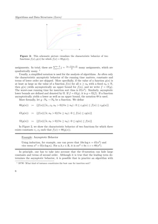
Example: Insertion Sort
5 2 3 6 1 4
2 5 3 6 1 4
2 3 5 6 1 4
2 3 5 6 1 4
1 2 3 5 6 4
1 2 3 4 5 6
Figure 1: Insertion sort for the sequence 5, 2, 3, 6, 1, 4 .
Intuitively, sorting 100 numbers takes longer than only 10 numbers. Therefore,
the running time is given as a function of the size of the input (n here). Furthermore,
for sequences of equal length, sorting ‘almost sorted’ sequences should be faster than
‘unsorted’ ones. Often, the so-called worst case running time of an algorithm is
studied as a function of the size of the input. The worst-case running time is the
largest possible running times for an instance of a certain size and yields an upper
bound for the running time of an arbitrary instance of the same size. It is not clear
beforehand whether the ‘worst case’ appears ‘often’ in practice or only represents some
‘unrealistic’, artificially constructed situation. For some applications, the worst case
appears regularly, for example when searching for a non-existing entry in a database.
For some algorithms, it is also possible to analyze the average case running time
which is the average over the time for all instances of the same size. Some algorithms
have a considerably better performance in the average than in the worst case, some
others do not. Often, however, it is difficult to answer the question what an ‘average
instance’ should be, and worst-case analyses are easier to perform. We now examine
the question whether the worst-case running time of insertion sort grows linearly,
or quadratically, or maybe even exponentially in n. First, suppose we are given a
sequence of n numbers, what constitutes the worst case for insertion sort? Clearly,
most work needs to be done when the instance is sorted, but in decreasing instead of
in increasing order. In this case, in each iteration the condition A[i] > key is always
satisfied and the while-loop only stops because the value of i drops to zero. Therefore,
for j = 2 one assignment A[i + 1] = A[i] has to be performed. For j = 3, two of these
assignments have to be done, and so on, until for j = n − 1 we have to perform n − 2
5

6. Algorithms and Data Structures (Liers)
c2g(x)
f(x)
c1g(x)
n0
Figure 2: This schematic picture visualizes the characteristic behavior of two
functions f(x), g(x) for which f(x) = Θ(g(x)).
assignments. In total, these are
n−2
j=1 j = (n−1)(n−2)
2 many assignments, which are
quadratically many. 1
Usually, a simplified notation is used for the analysis of algorithms. As often only
the characteristic asymptotic behavior of the running time matters, constants and
terms of lower order are skipped. More specifially, if the value of a function g(n) is
at least as large as the value of a function f(n) for all n ≥ n0 with a fixed n0 ∈ N,
then g(n) yields asymptotically an upper bound for f(n), and we write f = O(g).
The worst-case running time for insertion sort thus is O(n2
). Similarly, asymptotic
lower bounds are defined and denoted by Ω. If f = O(g), it is g = Ω(f). If a function
asymptotically yields a lower as well as an upper bound, the notation Θ is used.
More formally, let g : N0 → N0 be a function. We define
Θ(g(n)) := {f(n)|(∃c1, c2, n0 > 0)(∀n ≥ n0) : 0 ≤ c1g(n) ≤ f(n) ≤ c2g(n)}
O(g(n)) := {f(n)|(∃c, n0 > 0)(∀n ≥ n0) : 0 ≤ f(n) ≤ cg(n)}
Ω(g(n)) := {f(n)|(∃c, n0 > 0)(∀n ≥ n0) : 0 ≤ cg(n) ≤ f(n)}
In Figure 2, we show the characteristic behavior of two functions for which there
exists constants c1, c2 such that f(x) = Θ(g(x)).
Example: Asymptotic Behavior
Using induction, for example, one can prove that 10n log n = O(n2
) and
vice versa n2
= Ω(n log n). For a, b, c ∈ R, it is an2
+ bn + c = Θ(n2
).
In principle, one has to take into account that the O-notation can hide large
constants and terms of second order. Although it is true that the leading term de-
termines the asymptotic behavior, it is possible that in practice an algorithm with
1 BTW: What kind of instance constitutes the best case for insertion sort?
6

7. 2 Sorting
slightly larger asymptotic running time performs better than another algorithm with
better O-behavior.
It turns out that also the average-case running time of insertion sort is O(n2
).
We will see later that sorting algorithms with worst-case running time bounded by
O(n log n) exists. For large instances, they show better performance than insertion
sort. However, insertion sort can easily be implemented and for small instances is
very fast in practice.
2.2 Sorting using the Divide-and-Conquer Principle
A general algorithmic principle that can be applied for sorting consists in divide
and conquer. Loosely speaking, this approach consists in dividing the problem into
subproblems of the same kind, conquering the subproblems by recursive solution or
direct solution if they are small enough, and finally combining the solutions of the
subproblems to one for the original problem.
2.2.1 Merge Sort
The well-known merge sort algorithm specifies the divide and conquer principle as
follows. When merge sort is called for array A that stores a sequence of n numbers, it
is divided into two sequences of equal length. The same merge sort algorithm is then
called recursively for these two shorter sequences. For arrays of length one, nothing
has to be done. The sorted subsequences are then merged in a zip-fastener manner
which results in a sorted sequence of length equal to the sum of the lengths of the
subsequences. An example implementation in C is given in the following. The main
function is similar to the one for insertion sort and is omitted here. The constant
infinity is defined to be a large number. Then, merge sort(A,1,n) is the call for
sorting an array A with n elements. In the following merge sort implementation,
recursive calls to merge sort are performed for subsequences A[p],. . . , A[r]. In line
5, the position q of the middle element of the sequence is determined. merge sort is
called for the two sequences A[p],. . . , A[q] and A[q+1],. . . , A[r].
1void merge_sort(int* A, int p, int r)
2{
3 int q;
4 if (p < r) {
5 q = p + ((r - p) / 2);
6 merge_sort(A, p, q);
7 merge_sort(A, q + 1,r);
8 merge(A, p, q, r);
9 }
10}
In the following, the merge of two sequences A[p],. . .,A[q] and A[q+1],...,A[r]
is implemented. To this end, an additional array B is allocated in which the merged
sequence is stored. Denote by ai and aj the currently considered elements of each of
7

8. Algorithms and Data Structures (Liers)
the sequences that need to be merged in a zip-fastener manner. Always the smaller
of ai and aj is stored into B (lines 12 and 17). If an element from a subsequence is
inserted into B, its subsequent element is copied into ai (aj, resp.) (lines 14 and 19).
The merged sequence B is finally copied into array A in line 22.
1void merge(int* A, int p, int q, int r)
2{
3 int i, j, k, ai, aj;
4 int *B;
5 B = (int *) malloc((r - p + 2)*sizeof(int));
6 i = p;
7 j = q + 1;
8 ai = A[i];
9 aj = A[j];
10 for (k = 1; k <= r - p + 1; k++) {
11 if (ai < aj) {
12 B[k] = ai;
13 i++;
14 if (i <= q) ai = A[i]; else ai = infinity;
15 }
16 else {
17 B[k] = aj;
18 j++;
19 if (j <= r) aj = A[j]; else aj = infinity;
20 }
21 }
22 for (k = p; k <= r; k++) A[k] = B[k-p+1];
23 free(B);
24}
Mergesort is well suited for sorting massive amounts of data that do not fit into
main memory. Subsequences that do fit into main memory are sorted first and then
merged only in the end. It is therefore called an external sorting algorithm.
Without going into a high level of detail, let us analyze the worst-case running
time of merge sort. Suppose it is some function T(n). For ease of presentation, we
assume that n is a power of two, i.e., there exists r ∈ N such that n = 2r
. We note
that the middle of the subsequence can be determined in constant time. We then
need to sort two subsequences of size n
2 which takes time 2T(n
2 ). Due to the for-loop
in merge(), merging two subsequences of lengths n
2 takes time Θ(n). In total, the
function T(n) to be determined needs to satisfy the recurrence
T(n) =
Θ(1), for n = 1
2T n
2 + Θ(n), for n > 1
It can be shown that the recurrence is solved by T(n) = Θ(n log2 n). (As a test, in-
sert this function into the recurrence...) Thus, the worst-case running time O(n log n)
of merge sort is better than the quadratic worst-case running time of insertion sort.
8

9. 2 Sorting
1 7 9 2 4 8 3 5
1 7 9 2 4 8 3 5
1 7 9 2 4 8 3 5
1 7 9 2 4 8 3 5
1 7 2 9 4 8 3 5
1 2 7 9 3 4 5 8
1 2 3 4 5 7 8 9
Figure 3: Sorting a sequence of numbers with mergesort.
Example: Merge Sort
Suppose we want to sort the instance 1, 7, 9, 2, 4, 8, 3, 5 with merge sort.
First, the recursive calls to the function merge sort continues dividing
the sequence in the middle into subsequences until the subsequences only
contain one element. This is visualized in the top of Figure 3 by a top-
down procedure. Then merge always merges subsequences into a larger
sorted sequence in a zip-fastener manner. This is as well visualized on the
bottom of Figure 3.
Instead of sorting numbers only, we can easily extend whatever we have said until
now to more general sorting tasks in which we are given n data records s1, s2, . . . , sn
with keys k1, k2, . . . , kn. An ordering relation ‘≤’ is defined on the keys and we need
to find a permutation of the data such that the permuted data is sorted according
to the ordering relation, as we discuss next. For example, a record could consist of a
name of a person together with a telephone number. The task could be to sort the
records alphabetically. The keys are the people’s names, and the alphabetical order
is the ordering relation.
2.2.2 Quicksort
Quicksort is another divide-and-conquer sorting algorithm that is widely used in prac-
tice. For a sequence with length at most one, nothing is done. Otherwise, we take a
9

10. Algorithms and Data Structures (Liers)
specific element ai from the sequence, the so-called pivot element. Let us postpone for
the moment a discussion how such a pivot should be chosen. We aim at finding the
correct position for ai. To this end, we start from the left and search for an element
ak in the subsequence left of ai that is larger than ai. As we want to sort in increasing
order, the position of ak is wrong. Similarly, we start from the right and search for an
element al in the subsequence right of ai that is smaller than ai. Elements al and ak
then exchange their positions. If only one such element is found, it is exchanged with
ai. This is the only case in which ai may change its position. Note that ai will still be
the pivot. This procedure is continued until no further elements need to be exchanged.
Then ai is at the correct position, say t, because all elements in the subsequence to its
left are not larger and all elements in the subsequence to its right are not smaller than
ai. This is the division step. We are now left with the task of sorting two sequences
of lengths t − 1 and n − t. Quicksort is called recursively for these sequences (conquer
step). Finally, the subsequences are combined to a sorted sequence by simple concate-
nation. Obviously, the running time of quicksort depends on the choice of the pivot
element. If we are lucky, it is chosen such that the lengths of the subsequences are
always roughly half of the length of the currently considered sequence which means
that we are done after roughly log n division steps. In each step, we have to do Θ(n)
many comparisons. Therefore, the best-case running time of quicksort is Θ(n log n).
If we are unlucky, ai is always the smallest or always the largest element so that we
need linearly many division steps. Then, we need
n
i=1 i = n(n+1)
2 = Θ(n2
) many
comparisons which leads to quadratic running time in the worst case. It can be proven
that the average-case running time is bounded from above by O(n log n). Different
choices for the pivot have been suggested in the literature. For example, one can just
always use the ‘rightmost’ element. A C-implementation of quicksort with this choice
of the pivot element is given below. However, quicksort has quadratic running time
in the worst case. Despite the fact that the worst-case running time of quicksort is
worse than that of merge sort, it is still the sorting algorithm that is mostly used in
practice. One reason is that the worst case does not occur often so that the ‘typical’
running time is better than quadratic in n. In practice, merge sort is usually faster
than quicksort.
In the following C-implementation we slightly extend the task to sorting elements
that have a key and some information info. Sorting takes place with respect to key.
A struct item is defined accordingly. In the main routine, we read in the keys for
item A (for brevity, info values are not considered in this example implementation).
Initially, quick sort is called for A and positions 1 to n.
1#include <stdio.h>
2#include <stdlib.h>
3typedef int infotype;
4typedef struct{
5 int key;
6 infotype info;
7} item;
8
10

11. 2 Sorting
9main()
10{
11 int i,j,n;
12 item *A;
13 scanf("%d",&n);
14 A = (item *) malloc((n+1)*sizeof(item));
15 for (i=1; i<=n; i++) {
16 scanf("%d",&j);
17 A[i].key = j;
18 }
19 A[0].key = -1;
20 quick_sort(A,1,n);
21 for (i=1; i<=n; i++) printf("%5d",A[i].key);
22 printf("n");
23 free(A);
24}
Next, the implementation of function quick sort is given. In line 8, the pivot
element is taken as the rightmost element at position r. While we find elements that
need to be exchanged with the pivot element (line 9), we compare the pivot with
the elements in the sequence. In line 10, we start with i = l and increase i until
the element at position i is at least as large as the pivot and thus should exchange
position with another element. Similarly, we start in line 11 with j = r and decrease
j until the element at position j is at most as large as the pivot. If position i is left
of j, the corresponding elements exchange position (lines 12–14). Otherwise, only
one element was found that has to be exchanged with the pivot (lines 18–20). The
while-loop stops when no further elements need to be exchanged and thus the pivot is
at the correct position. Then, quick sort is called recursively for the subsequences
A[l],. . ., A[i-1] and A[i+1],. . ., A[r] in lines 21 and 22.
1void quick_sort(item* A, int l, int r)
2{
3 int i,j,pivot;
4 item t;
5 if (r>l) {
6 i = l - 1;
7 j = r;
8 pivot = A[r].key; /* pivot element */
9 while (1) {
10 do i++; while (A[i].key < pivot);
11 do j--; while (A[j].key > pivot);
12 if(i >= j) break; /* i is position of pivot */
13 t = A[i];
14 A[i] = A[j];
15 A[j] = t;
16 }
17 t = A[i];
18 A[i] = A[r];
11

12. Algorithms and Data Structures (Liers)
19 A[r] = t;
20 quick_sort(A,l,i-1);
21 quick_sort(A,i+1,r);
22 }
23}
2.3 A Lower Bound on the Performance of Sorting Algorithms
The above methods can be applied if we are given the sequence of numbers that needs
to be sorted without further information. In case, for example, it is known that the n
numbers are taken from a set of elements with bounded size, there exists algorithms
that can sort these sequences in a more efficient way. For example, if it is known that
the numbers are taken from the set of {1, . . . , nk
}, then bucket sort can sort them in
time O(kn). In contrast, for the algorithms considered here, the only information we
have is based on comparing the elements’ keys.
Suppose we want to design a sorting algorithm that sorts arbitrary sequences of
n elements. It is only based on comparing their keys and on moving data records.
Considering sequences with pairwise different elements, it can be proven that any
sorting algorithm has a running time bounded from below by Ω(n log n). As we
cannot achieve a comparison based-algorithm with better running time than that,
merge sort is a sorting algorithm that is asymptotically time-optimal. The same is
true for the heap sort method that we do not cover in this introductory chapter.
3 Select the k-th smallest element
Suppose we want to find the k-th smallest number in a (potentially unsorted) sequence
of numbers. As a special case, if n is odd and k = n+1
2 , we want to find the median
of the sequence. For the special case of determining the minimum (maximum, resp.)
element, we simply scan once through the list in linear time, compare the scanned
element with the currently smallest (largest, resp.) element and update the latter
whenever necessary.
For general values of k, a straightforward solution for searching the k-th element
in sorted order is: We first sort the n numbers in time O(n log n) and then find the
k element. The total running time of this algorithm is bounded by the sorting step
and thus needs time O(n log n) in the worst case. This approach is a good choice
if many selection queries need to be performed as these queries are fast once the
sequence is sorted. There exist however also algorithms with linear running time, for
example the median of medians algorithm. Its general idea is closely related to that
of quicksort in the sense that a pivot element is determined, pairs of elements are
swapped appropriately and then the problem is solved recursively for a subsequence.
The pivot element is determined by dividing the n elements into groups of five elements
each (plus zero to four leftover elements). The elements in each group are sorted and
their median is taken. In total, this yields n
5 ‘median’ elements. In this subsequence
of medians, the median is determined recursively using the same grouping algorithm.
12

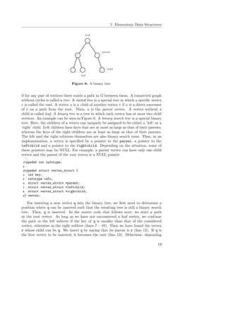
13. 4 Binary Search
The resulting ‘median of medians’ is taken as pivot element with the same role as
in quicksort. The sequence is then divided into two subsequences according to the
position of the pivot. The search is continued recursively in the correct subsequence
of the two until the position of the pivot is k and the algorithm stops. It can be
proven that the worst-case running time of this algorithm is bounded by O(n).
4 Binary Search
Suppose we have some sorted sequence at hand and want to know the position of an
element with a certain key k. For example, let the keys be 1, 3, 3, 7, 9, 15, 27 . Suppose
we want to determine the position of an element with key 9. A straightforward linear-
time search algorithm would scan each element in the sequence, compare it with the
element we search for and stops when either the element we look for has been found
or the whole sequence has been scanned without success. If we however know that
the sequence is sorted, searching for a specific element can be done more efficently
with the divide and conquer principle.
Suppose, for example, we want to find the telephone number of a specific person
in a telephone book. Usually, people do a mixture of a divide and conquer method
together with a linear search. In fact, if we look for a person with name Knuth, we
will open the telephone book somewhere in the middle. If the names of the people
where we opened start, say, with an O instead a K, we know we need to search for
Knuth further towards the beginning of the boook. If instead they start with, say,
an F, we need to search further towards the end. If we find that at the beginning of
the current page, the names are ‘close’ to Knuth, we probably continue with a linear
search until we find Knuth.
A more formalized search algorithm using divide and conquer, binary search, needs
only time O(log n) in the worst case. We just compare k with the key of the element
in the middle of the currently considered sorted sequence. If this key is the one we are
searching for, we stop. Otherwise, if the key is smaller than k, we know we have to
search in the subsequence ‘left of the middle’ that contains the elements with smaller
keys. If instead it is larger, the element we look for is in the subsequence right of the
middle. We apply the same argument in the corresponding subsequence whose length
is half of that of the original one. An implementation of binary search is given next.
First, we specify the main function.
Next, the implementation of binary search is given. The middle m of the sequence
A[l],. . ., A[r] is determined in line 7. If the element at this position is smaller than
k (line 8), we continue the search in the subsequence A[l],. . ., A[m-1], otherwise
in A[m+1],. . ., A[r] (line 8 and 9). The search stops either if the element has been
found or when the lower index l has become at least as large as the upper r (line 10)
which means that k is not contained in the sequence.
1int binary_search(item *A, int l, int r, int k)
2/* searches for position with key k in A[l..r], */
3/* returns 0, if not successful */
13

14. Algorithms and Data Structures (Liers)
4{
5 int m;
6 do {
7 m = l + ((r - l) / 2);
8 if (k<A[m].key) r = m - 1;
9 else l = m + 1;
10 } while ((k!=A[m].key) && (l<=r));
11 if (k==A[m].key) return m;
12 else return 0;
13}
For simplifying the analysis, we assume that the length of the sequence is a power
of two minus 1, i.e., n can be written as n = 2r
− 1 with some appropriately chosen
r ∈ N. We need constant time for determining the middle of the sequence and for
the decision whether we need to continue the search in the subsequence to the left or
in that to the right. In the best case, we immediately find the correct element and
thus have a best-case running time of Θ(1). In the worst case, the element we look
for is either not contained in the sequence or is only found when the subsequence has
length one. Then, log n division steps and decisions for the correct subsequences have
to be performed. As each of these steps needs constant time, the worst-case running
time of binary search is Θ(log n). (One can show that also the average-case running
time is Θ(log n).)
Example: Binary Search
Consider again the sequence 1, 3, 3, 7, 9, 15, 27 . Suppose we want to de-
termine the position of an element with key k = 3. First, binary search
compares the middle element (key equal to 7) with k. As k < 7, the search
continues in the subsequence 1, 3, 3 . The middle of this subsequence is
then an element we look for and we can stop.
5 Elementary Data Structures
Up to now, we have mainly focused on sorting algorithms and their performance. In
the given C implementations, the elements were simply stored in arrays of length
n. Whereas arrays are well suited for our purposes, it is sometimes necessary to use
more involved data structures. As an easy example, suppose we have an application in
which we do not know beforehand how many elements we need to store. Or suppose
we want to remove an element somewhere in the middle. Of course, when using an
array, elements can be deleted from it by shifting all elements further ‘right’ one
position to the left. This however can take long for large n and many deletion tasks
as one deletion operation needs a time that grows linearly with the size of the array,
in the worst case. Furthermore, inserting an element into an array usually means to
copy the whole array into a new one that is larger. Therefore, more advanced data
structures have been introduced that serve different purposes.
14

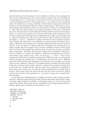
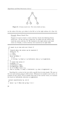
15. 5 Elementary Data Structures
push pop
Figure 4: A visualization of a stack.
5.1 Stacks
As an elementary data structure, we introduce a stack. A stack works like an in-tray
that people use for incoming mail in the sense that whatever is inserted last is returned
first (‘last-in first-out’ principle), see Figure 4. As elementary operations, a stack has
several functions available. The function empty returns 0, if no element is contained
in it, and 1 otherwise. Similarly, full also returns a Boolean value. push inserts
an element in the stack and pop deletes and returns the element that was inserted
last. As elements are only inserted and deleted at one ‘end’, a stack can easily be
implemented with an array of a maximum size that is given by STACKSIZE. Here,
elements are inserted and deleted from the ‘right’. In the following main function, the
stack is initialized (line 12). As an example, some elements are pushed into it and
finally removed again (lines 13–19). The last pop operation simply returns a message
saying the stack is empty.
1#include <stdio.h>
2#include <stdlib.h>
3#define STACKSIZE 4
4
5typedef struct {
6 int stack[STACKSIZE-1];
7 int stackpointer;
8} Stackstruct;
9
10void stackinit(Stackstruct* s);
11int empty(Stackstruct* s);
12int full(Stackstruct* s);
13void push(Stackstruct* s, int v);
14int pop(Stackstruct* s);
15
16main()
17{
18 Stackstruct s;
19 stackinit(&s);
20 push(&s,1);
21 push(&s,2);
15

16. Algorithms and Data Structures (Liers)
22 push(&s,3);
23 printf("%dn",pop(&s));
24 printf("%dn",pop(&s));
25 printf("%dn",pop(&s));
26 printf("%dn",pop(&s));
27}
Next, the implementation of the stack functions is given. The variable stackpointer
stores the number of elements contained in the stack. In stackinit, this variable is
set to zero. In push, an element is inserted in the stack by inserting it into the array
at position stackpointer. pop then returns the element at position stackpointer
and ‘deletes’ the popped element by reducing the size of stackpointer by one.
1void stackinit(Stackstruct *s)
2{
3 s->stackpointer = 0;
4}
5
6int empty(Stackstruct *s)
7{
8 return (s->stackpointer<=0);
9}
10
11int full(Stackstruct *s)
12{
13 return (s->stackpointer>=STACKSIZE);
14}
15
16void push(Stackstruct *s, int v)
17{
18 if (full(s)) printf("!!! Stack is full !!!n");
19 else {
20 s->stack[s->stackpointer] = v;
21 s->stackpointer++;
22 }
23}
24
25int pop(Stackstruct *s)
26{
27 if (empty(s)) {
28 printf("!!! Stack is empty !!!n");
29 return -1;
30 }
31 else {
32 s->stackpointer--;
33 return s->stack[s->stackpointer];
34 }
35}
16

17. 5 Elementary Data Structures
1 5 2 9
Figure 5: A singly-linked list.
1 5 2 9
11
Figure 6: Inserting an item into a singly-linked list.
Stacks are used, for example in modern programming languages. The compilers that
translate the source code of a formal language to an executable and languages like
Postscript entirely rely on stacks.
5.2 Linked Lists
If the number of records that need to be stored is not known beforehand, a list can be
used. Each record (also called node) in the list has a link to its successor in the list.
(The last element links to a NULL record.) We also save a pointer head to the start of
the list. A visualization of such a singly-linked list can be seen in Figure 5. Inserting
a record into and deleting a record from the list can then be done in constant time
by manipulating the corresponding links. If for each element there is an additional
link to the predecessor in the list, we say the list is doubly-linked.
The implementation of a node in the list consists of an item as implemented
before, together with a link pointer to its successor that is called next.
1typedef struct Node_struct {
2 item dat;
3 struct Node_struct *next;
4} Node;
If a new item is inserted into the list next to some Node p, we first store it into a
new Node that we call r. Then, the successor of p is r (line 1 in the following source
code) , and the successor of r is q (line 2). In C, this looks as follows.
1 Node *q = p->next;
2 p->next = r;
3 r->next = q;
Deleting the node next to p can be performed as follows. We first link p->next to
p->next->next, see Figure 6. We then free the memory of p. (Here, we assume we
are already given p. In case we instead only know, say, the key of the Node we want
to remove, we first need to search for the Node with this key.)
17

18. Algorithms and Data Structures (Liers)
1 5 2
11
Figure 7: Deleting the node with key 9 from the singly-linked list.
1 Node *r = p->next;
2 p->next = p->next->next;
3 free(r);
Finally, we want to search for a specific item x in the list. This can easily be done
with a while-loop that starts at the beginning of the list and continues comparing the
nodes in the list with the element. While the correct element has not been found, the
next element is considered.
1 Node *pos = head;
2 while (pos != NULL && pos->next->dat.key != x.key ) pos = pos->next;
3 return pos;
Other advanced data structures exists, for example queues, priority queues, and
heaps. For each application, a different data structure might work best. Therefore,
one first specifies the necessary functionality and then decides which data structure
serves the needs. Here, let us briefly compare an array with a singly-linked linear
list. When using an array A, accessing an element at a certain position i can be done
in constant time by accessing A[i]. In contrast, a list does not have indices, and
indexing takes O(n). Inserting an element in an array or deleting it needs time O(n)
as discussed above, whereas it takes constant time in a linked list if inserted at the
beginning or at the end. If the node is not known next to which it has to be inserted,
insertion takes the time for searching the corresponding node plus constant time for
manipulating the links. Thus, depending on the application, a list can be suited
better than an array or vice versa. The sorting algorithms that we have introduced
earlier make frequent use of accessing elements at certain positions. Here, an array is
suited better than a list.
5.3 Graphs, Trees, and Binary Search Trees
A graph is a tuple G = (V, E) with a set of vertices V and a set of edges E ⊆ V × V .
An edge e (also denoted by its endpoints (u, v)) can have a weight we ∈ R. Then
the graph is called weighted. Graphs are used to represent elements (vertices) with
pairwise relations (edges). For example, the street map of Germany can be represented
by vertices for each city and an edge between each pair of cities. The edge weights
denote the travel distance between the corresponding cities. A task could then be, for
example, to determine the shortest travel distance between Oldenburg and Cologne.
A sequence of vertices v1, . . . , vp in which subsequent vertices are connected by an edge
is called a path. If v1 = vp, we say the path is a cycle. A graph is called connected
18

19. 5 Elementary Data Structures
root
parent
child
leaf
Figure 8: A binary tree.
if for any pair of vertices there exists a path in G between them. A connected graph
without cycles is called a tree. A rooted tree is a special tree in which a specific vertex
r is called the root. A vertex u is a child of another vertex v if u is a direct successor
of v on a path from the root. Then, u is the parent vertex. A vertex without a
child is called leaf. A binary tree is a tree in which each vertex has at most two child
vertices. An example can be seen in Figure 8. A binary search tree is a special binary
tree. Here, the children of a vertex can uniquely be assigned to be either a ‘left’ or a
‘right’ child. Left children have keys that are at most as large as that of their parents,
whereas the keys of the right children are at least as large as that of their parents.
The left and the right subtrees themselves are also binary search trees. Thus, in an
implementation, a vertex is specified by a pointer to the parent, a pointer to the
leftchild and a pointer to the rightchild. Depending on the situation, some of
these pointers may be NULL. For example, a parent vertex can have only one child
vertex and the parent of the root vertex is a NULL pointer.
1typedef int infotype;
2
3typedef struct vertex_struct {
4 int key;
5 infotype info;
6 struct vertex_struct *parent;
7 struct vertex_struct *leftchild;
8 struct vertex_struct *rightchild;
9} vertex;
For inserting a new vertex q into the binary tree, we first need to determine a
position where q can be inserted such that the resulting tree is still a binary search
tree. Then, q is inserted. In the source code that follows next, we start a path
at the root vertex. As long as we have not encountered a leaf vertex, we continue
the path in the left subtree if the key of q is smaller than that of the considered
vertex, otherwise in the right subtree (lines 7 – 10). Then we have found the vertex
r whose child can be q. We insert q by saying that its parent is r (line 12). If q is
the first vertex to be inserted, it becomes the root (line 13). Otherwise, depending
19

20. Algorithms and Data Structures (Liers)
17
10
5 12
19
21
Figure 9: A binary search tree. The vertex labels are keys.
on the value of its key, q is either in the left or in the right subtree of r (line 14).
Example: Binary Search Tree
Suppose we want to insert a vertex with key 13 into the following binary
search tree. As the root has a larger key, we follow the left subtree and
reach the vertex with key 10. We continue in the right subtree and reach
vertex 12. Finally, a vertex with key 13 is inserted as its right child.
1/* insert *q in tree with root **root */
2{
3 /*search where the vertex can be inserted */
4 vertex *p, *r;
5 r = NULL;
6 p = *root;
7 while (p!=NULL) {
8 r = p;
9 if (q->key < p->key) p = p->leftchild; else p = p->rightchild;
10 }
11 /* insert the vertex */
12 q->parent = r;
13 q->leftchild = NULL;
14 q->rightchild = NULL;
15 if (r == NULL) *root = q;
16 else if (q->key < r->key) r->leftchild = q; else r->rightchild = q;
Searching for a vertex in the tree with a specific key k is also simple. We start at
the root and continue going to child vertices. Whenever we consider a new vertex, we
compare its key with k. If k is smaller than that of the current vertex, we continue
the search at leftchild, otherwise at rightchild.
1vertex* search(vertex *p, int k)
2{
3 while ( (p != NULL) && (p->key != k) )
20

21. 6 Advanced Programming
4 if (k < p->key) p = p->leftchild; else p = p->rightchild;
5 return p;
6}
The search for the element with minimum (maximum, resp.) key can then be
performed by starting a path from the root, ending at the ‘leftmost’ (‘rightmost’,
resp.) leaf. In source code, the search for the minimum looks as follows.
1vertex* minimum(vertex *p)
2{
3 while (p->leftchild != NULL) p = p->leftchild;
4 return p;
5}
6 Advanced Programming
In practice, it is of utmost importance to have fast algorithms with good worst-case
performance at hand. Additionally, they need to be implemented efficiently. Further-
more, a careful documentation of the source code is indispensable for debugging and
maintaining purposes.
Elementary algorithms and data structures such as those introduced in this chap-
ter are used quite often in larger software projects. Both from a performance and
from a software-reusability point of view, they are often not implemented by the
programmer. Instead, fast implementations are used that are available in software
libraries. The standard C library stdlib implements, among other things, differ-
ent input and output methods, mathematical functions, quicksort and binary search.
For data structures and algorithms, (C++) libraries such as LEDA [6], boost[2], or
OGDF[4] exist. For linear algebra functions, the libraries BLAS[1] and LAPACK[3]
can be used.
Acknowledgments
Financial support by the DFG is acknowledged through project Li1675/1. The
author is grateful to Michael J¨unger for providing C implementations of the pre-
sented algorithms and some variants of implementations for the presented data struc-
tures. Thanks to Gregor Pardella and Andreas Schmutzer for critically reading this
manuscript.
6.1 References
References
[1] Blas (basic linear algebra subprograms). http://www.netlib.org/blas/.
[2] boost c++ libraries. http://www.boost.org/.
21

22. Algorithms and Data Structures (Liers)
[3] Lapack – linear algebra package. http://www.netlib.org/lapack/.
[4] Ogdf - open graph drawing framework. http://www.ogdf.net.
[5] Thomas H. Cormen, Charles E. Leiserson, Ronald L. Rivest, and Clifford Stein.
Introduction to algorithms. MIT Press, Cambridge, MA, third edition, 2009.
[6] Algorithmic Solutions Software GmbH. Leda. http://www.algorithmic-
solutions.com/leda/.
[7] Donald E. Knuth. The art of computer programming. Vol. 3: Sorting and Search-
ing. Addison-Wesley, Upper Saddle River, NJ, 1998.
[8] Robert Sedgewick. Algorithms in C Parts 1-4: Fundamentals, Data Structures,
Sorting, Searching. Addison-Wesley Professional, third edition, 1997.
22