Documentation new perspectives excel 2019 module 9 sam project 1

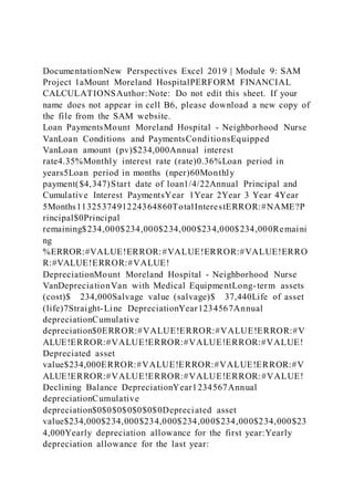
1. DocumentationNew Perspectives Excel 2019 | Module 9: SAM
Project 1aMount Moreland HospitalPERFORM FINANCIAL
CALCULATIONSAuthor:Note: Do not edit this sheet. If your
name does not appear in cell B6, please download a new copy of
the file from the SAM website.
Loan PaymentsMount Moreland Hospital - Neighborhood Nurse
VanLoan Conditions and PaymentsConditionsEquipped
VanLoan amount (pv)$234,000Annual interest
rate4.35%Monthly interest rate (rate)0.36%Loan period in
years5Loan period in months (nper)60Monthly
payment($4,347)Start date of loan1/4/22Annual Principal and
Cumulative Interest PaymentsYear 1Year 2Year 3 Year 4Year
5Months1132537491224364860TotalInterestERROR:#NAME?P
rincipal$0Principal
remaining$234,000$234,000$234,000$234,000$234,000Remaini
ng
%ERROR:#VALUE!ERROR:#VALUE!ERROR:#VALUE!ERRO
R:#VALUE!ERROR:#VALUE!
DepreciationMount Moreland Hospital - Neighborhood Nurse
VanDepreciationVan with Medical EquipmentLong-term assets
(cost)$ 234,000Salvage value (salvage)$ 37,440Life of asset
(life)7Straight-Line DepreciationYear1234567Annual
depreciationCumulative
depreciation$0ERROR:#VALUE!ERROR:#VALUE!ERROR:#V
ALUE!ERROR:#VALUE!ERROR:#VALUE!ERROR:#VALUE!
Depreciated asset
value$234,000ERROR:#VALUE!ERROR:#VALUE!ERROR:#V
ALUE!ERROR:#VALUE!ERROR:#VALUE!ERROR:#VALUE!
Declining Balance DepreciationYear1234567Annual
depreciationCumulative
depreciation$0$0$0$0$0$0$0Depreciated asset
value$234,000$234,000$234,000$234,000$234,000$234,000$23
4,000Yearly depreciation allowance for the first year:Yearly
depreciation allowance for the last year:

2. Earnings ProjectionsMount Moreland Hospital - Neighborhood
Nurse VanEarnings
ProjectionsIncome20222023202420252026Municipal grants$
25,000$ 40,000Federal
grants72,00058,00058,00055,00055,000Insurance
reimbursements345,000550,000Total Revenue$ 442,000$
58,000$ 58,000$ 55,000$ 645,000ExpensesSupplies$
108,000$ 110,000$ 112,000$ 115,000$
118,000Pharmaceuticals127,000129,625132,250134,875137,500
Payroll140,000Maintenance2,5002,5002,5003,0003,000Insuranc
e2,8002,8002,8003,1003,100Advertising10,50010,50010,50010,
50010,500Total General Expenses$ 390,800$ 255,425$
260,050$ 266,475$ 272,100Initial Earnings$ 51,200$
(197,425)$ (202,050)$ (211,475)$ 372,900
Projected Revenue
44562 44927 45292 45658 46023 442000
58000 58000 55000 645000
Income
Revenue Trend
Revenue 1 2 3 4 5 6 7 8 9 10 11
12 13 14 15 16 17 18 19 20 21 22 23
24 25 26 27 28 29 30 31 32 33 34 35
36 37 38 39 40 41 42 43 44 45 46 47
48 49 50 51 52 53 54 55 56 57 58 59
60 29443 33967 34268 37665 38775
36834 31995 36935 38021 38566 38775
38756 36012 37345 39552 40207 40113
39765 30599 40215 41750 42154 40205
40450 41599 42702 42998 40012 44175
44998 44765 41248 45060 45621 45987

3. 49958 48155 48014 49109 49121 49342
45695 44992 47622 48252 49013 49211
50001 50225 50100 51225 50026 51245
50875 49765 51232 53012 53187 54675
53412
Months in Operation
Revenue
Monthly Revenue ProjectionsMonthMonth NumberRevenueJan
2022129,443Feb 2022233,967Mar 2022334,268Apr
2022437,665May 2022538,775Jun 2022636,834Jul
2022731,995Aug 2022836,935Sep 2022938,021Oct
20221038,566Nov 20221138,775Dec 20221238,756Jan
20231336,012Feb 20231437,345Mar 20231539,552Apr
20231640,207May 20231740,113Jun 20231839,765Jul
20231930,599Aug 20232040,215Sep 20232141,750Oct
20232242,154Nov 20232340,205Dec 20232440,450Jan
20242541,599Feb 20242642,702Mar 20242742,998Apr
20242840,012May 20242944,175Jun 20243044,998Jul
20243144,765Aug 20243241,248Sep 20243345,060Oct
20243445,621Nov 20243545,987Dec 20243649,958Jan
20253748,155Feb 20253848,014Mar 20253949,109Apr
20254049,121May 20254149,342Jun 20254245,695Jul
20254344,992Aug 20254447,622Sep 20254548,252Oct
20254649,013Nov 20254749,211Dec 20254850,001Jan
20264950,225Feb 20265050,100Mar 20265151,225Apr
20265250,026May 20265351,245Jun 20265450,875Jul
20265549,765Aug 20265651,232Sep 20265753,012Oct
20265853,187Nov 20265954,675Dec 20266053,412
InvestmentMount Moreland Hospital - Neighborhood Nurse
VanInvestment ReturnsInvestor Repayment
SchedulePaymentsNet Cash FlowStartup$ (165,000)$

4. (165,000)Year 125,000(140,000)Year 232,500(107,500)Year
335,500(72,000)Year 440,500(31,500)Year 541,50010,000Year
640,00050,000Desired rate of return7.30%Present valueNet
present value$ (165,000)Internal rate of return
Elements of Job Design and their Impact on the Organization
Function of Management
By <Your name here>
This document does not contain Technical Data or Technology
as defined in the ITAR Part 120.10 or EAR Part 772
This presentation will answer the question:
Job Enlargement
Job Enrichment
Job Rotation
Job Satisfaction?
Productivity?
Motivation?
How do ELEMENTS
Impact

5. This document does not contain Technical Data or Technology
as defined in the ITAR Part 120.10 or EAR Part 772
New Perspectives Excel 2019 | Module 9: SAM Project 1a
Mount Moreland Hospital
New Perspectives Excel 2019 | Module 9: SAM Project 1a
PERFORM FINANCIAL CALCULATIONS
PROJECT STEPS
Pranjali Kashyap is a financial analyst at Mount Moreland
Hospital in Baltimore, Maryland. She is using an Excel
workbook to analyze the financial data for a proposed program
called Neighborhood Nurse. The program involves nurses and
nurse practitioners providing healthcare services to Baltimore
neighborhoods from a van outfitted with medical equipment and
supplies. She asks for your help in correcting errors and making
financial calculations in the workbook.
Go to the Loan Payments worksheet. The hospital needs a loan
to buy the medical van for the Neighborhood Nurse program.
Before Pranjali can calculate the principal and interest
payments on the loan, she asks you to correct the errors in the
worksheet. Correct the first error as follows:
In cell H17, use the Error Checking command to identify the
error in the cell.
Correct the error to total the values in the range C17:G17. In a
later step, you will calculate the interest and principal in the
range C17:G18 to remove the remaining errors.

6. Correct the #VALUE! errors in the worksheet as follows:
Use Trace Precedents arrows to find the source of the #VALUE!
error in cell C20.
Correct the formula in cell C20, which should divide the
remaining principal (cell C19) by the loan amount (cell D5) to
find the percentage of remaining principal.
Fill the range D20:G20 with the formula in cell C20 to correct
the remaining #VALUE! errors.
Remove any remaining trace arrows.
Now Pranjali is ready to calculate the annual principal and
interest payments for the medical van. Start by calculating the
cumulative interest payments as follows:
In cell C17, enter a formula using the CUMIPMT functio n to
calculate the cumulative interest paid on the loan for Year 1
(payment 1 in cell C15 through payment 12 in cell C16). Use 0
as the type argument in your formula because payments are
made at the end of the period.
Use absolute references for the rate, nper, and pv arguments,
which are listed in the range D5:D11.
Use relative references for the start and end arguments.
Fill the range D17:G17 with the formula in cell C17 to calculate
the interest paid in Years 2–5 and the total interest.
Calculate the cumulative principal payments as follows:
In cell C18, enter a formula using the CUMPRINC function to
calculate the cumulative principal paid for Year 1 (payment 1 in
cell C15 through payment 12 in cell C16). Use 0 as the type
argument in your formula because payments are made at the end
of the period.
Use absolute references for the rate, nper, and pv arguments,
which are listed in the range D5:D11.
Use relative references for the start and end arguments.
Fill the range D18:G18 with the formula in cell C18 to calculate
the principal paid in Years 2–5 and the total principal.
Go to the Depreciation worksheet. Pranjali needs to correct the
errors on this worksheet before she can perform any
depreciation calculations.

7. Correct the errors as follows:
Use Trace Dependents arrows to determine whether the
#VALUE! error in cell D12 is causing the other errors in the
worksheet.
Use Trace Precedents arrows to find the source of the error in
cell D12.
Correct the error so that the formula in cell D12 calculates the
cumulative straight-line depreciation of the medical van by
adding the Cumulative depreciation value in Year 1 to the
Annual depreciation value in Year 2.
Pranjali wants to compare straight-line depreciation amounts
with declining balance depreciation amounts to determine which
method is more favorable for the hospital's balance sheet. In the
range D5:D7, she estimates that the Neighborhood Nurse
program will have $234,000 in tangible assets at startup, and
that the useful life of these assets is seven years with a salvage
value of $37,440.
Start by calculating the straight-line depreciation amounts as
follows:
In cell C11, enter a formula using the SLN function to calculate
the straight-line depreciation for the medical van during its first
year of operation.
Use absolute references for the cost, salvage, and life arguments
in the SLN formula.
Fill the range D11:I11 with the formula in cell C11 to calculate
the annual and cumulative straight-line depreciation in Years 2–
7.
Calculate the declining balance depreciation amounts for the
medical van as follows:
In cell C18, enter a formula using the DB function to calculate
the declining balance depreciation for the medical van during its
first year of operation.
Use Year 1 (cell C17) as the current period.
Use absolute references only for the cost, salvage, and life
arguments in the DB formula.
Fill the range D18:I18 with the formula in cell C18 to calculate

8. the annual and cumulative declining balance depreciation in
Years 2–7.
Pranjali also wants to determine the depreciation balance for the
first year and the last year of the useful life of the medical van.
Determine these amounts as follows:
In cell E22, enter a formula using the SYD function to calculate
the depreciation balance for the first year.
Use Year 1 (cell C17) as the current period.
In cell E23, enter a formula using the SYD function to calculate
the depreciation balance for the last year.
Use Year 7 (cell I17) as the current period.
Go to the Earnings Projections worksheet. Pranjali has entered
most of the income and expense data on the worksheet. She
knows the income from municipal grants will be $25,000 in
2022, and estimates it will be $40,000 in 2026. She needs to
calculate the income from municipal grants in the years 2023–
2025. The grants should increase at a constant amount from year
to year.
Project the income from Municipal grants for 2023–2025 (cells
D5:F5) using a Linear Trend interpolation.
Pranjali also needs to calculate the income from insurance
reimbursements in the years 2023–2025. She knows the starting
amount and has estimated the amount in 2026. She thinks this
income will increase by a constant percentage.
Project the income from Insurance reimbursements for 2023–
2025 (cells D7:F7) using a Growth Trend interpolation.
Pranjali needs to calculate the payroll expenses in the years
2023–2026. She knows the payroll will be $140,000 in 2022 and
will increase by at least five percent per year.
Project the payroll expenses as follows:
Project the expenses for Payroll for 2023-2026 (cells D13:G13)
using a Growth Trend extrapolation.
Use 1.05 (a 5 percent increase) as the step value.
The Projected Revenue line chart in the range H4:Q19 shows
the revenue Pranjali estimates in the years 2022–2026. She
wants to extend the projection into 2027.

9. Modify the Projected Revenue line chart as follows to forecast
the future trend:
Add a Linear Trendline to the Projected Revenue line chart.
Format the trendline to forecast 1 period forward.
The Revenue Trend scatter chart in the range A21:G40 is based
on monthly revenue estimates listed on the Monthly Revenue
Projections worksheet. Pranjali wants to include a trendline for
this chart that shows how revenues increase quickly at first and
then level off in later months.
Modify the Revenue Trend scatter chart as follows to include a
logarithmic trendline:
Add a Trendline to the Revenue Trend scatter chart.
Format the trendline to use the Logarithmic option.
Go to the Investment worksheet. This worksheet should show
the returns potential investors could realize if they invested
$165,000 in the Neighborhood Nurse program. Pranjali figures a
desirable rate of return would be 7.3 percent. She estimates the
investment would pay different amounts each year (range
C7:C12) and wants to calculate the present value of the
investment.
Calculate the present value of the investment as follows:
In cell C15, enter a formula that uses the NPV function to
calculate the present value of the investment in a medical van
for the Neighborhood Nurse program.
Use the desired rate of return value (cell C14) as the rate
argument.
Use the payments in Years 1–6 (range C7:C12) as the returns
paid to investors. (Hint: If a Formula Omits Adjacent Cell error
warning appears, ignore it.)
Pranjali also wants to calculate the internal rate of return on the
investment. If it is 7 percent or higher, she is confident she can
attract investors.
Calculate the internal rate of return on the investment as
follows:
In cell C17, enter a formula that uses the IRR function to
calculate the internal rate of return for investing in a medical

10. van for the Neighborhood Nurse program.
Use the payments for startup and Years 1–6 (range C6:C12) as
the returns paid to investors.
Your workbook should look like the Final Figures on the
following pages. Save your changes, close the workbook, and
then exit Excel. Follow the directions on the SAM website to
submit your completed project.
Final Figure 1: Loan Payments Worksheet
Final Figure 2: Depreciation Worksheet
Final Figure 3: Earnings Projections Worksheet
Final Figure 4: Monthly Revenue Projections Worksheet
Final Figure 5: Investment Worksheet
2