Inter-annual variability of currents and water properties offshore of the mid-Atlantic bight
•
0 likes•309 views

Inter-annual variability of currents and water properties offshore of the mid-Atlantic bight Charlie Flagg (SBU)-Kathy Donohue (GSO)-Jon Hare (NMFS) URI Climate Change Science Symposium - May 5, 2011

Recommended
Recommended
More Related Content
Viewers also liked
Viewers also liked (6)
Similar to Inter-annual variability of currents and water properties offshore of the mid-Atlantic bight
Similar to Inter-annual variability of currents and water properties offshore of the mid-Atlantic bight (20)
More from riseagrant
More from riseagrant (20)
Recently uploaded
Recently uploaded (20)
Inter-annual variability of currents and water properties offshore of the mid-Atlantic bight
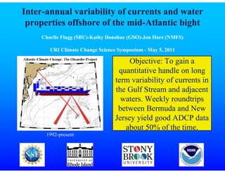
- 1. Inter-annual variability of currents and water properties offshore of the mid-Atlantic bight Charlie Flagg (SBU)-Kathy Donohue (GSO)-Jon Hare (NMFS) URI Climate Change Science Symposium - May 5, 2011 Objective: To gain a quantitative handle on long term variability of currents in the Gulf Stream and adjacent waters. Weekly roundtrips between Bermuda and New Jersey yield good ADCP data about 50% of the time. 1992-present
- 2. Acoustic remote sensing - currents The 75 kHz ADCP can reach to 600-700 m depth in good weather and in the absence of bubbles blocking the beams. This figure highlights the vertical coherence of the Gulf Stream, and the westward flow in the Slope and Sargasso Seas. cont. slo pe
- 3. Acoustic remote sensing - biology The Gulf Stream Slope Sea Sargasso Sea Top: currents (m/s). Bottom: raw backscatter count (not range corrected) - a measure of particle density.
- 4. Acoustic remote sensing - biology The Gulf Stream Slope Sea Sargasso Sea Top: currents (m/s). Bottom: raw backscatter count (not range corrected) - a measure of particle density. Note multiple - DSL - layers of diurnal migration - deep scattering layer and complexity in the Gulf Stream.
- 5. A typical transit A very unusual transit CCR AVHRR SST from http://fermi.jhuapl.edu/avhrr/gs (excellent website)
- 6. Hovmöller diagram of velocity (m/s) in 67°T from shelfbreak to Bermuda. Note lateral shifting of the GS. ea op eS m Sl trea lf S Gu 1 m/s 1 J/kg ea oS ass Sarg Warm colors to the NE, cool colors the west east the SW. Heavy line = 0 m/s. The ‘beaded’ structure of the GS due to meandering.
- 7. Directly measured transports Seasonal variation in GS transport. The 15% scatter is the reason frequent 4.3% sampling is crucial to (JMR - July 2010) construct means and their LF variability. The 3 subzones exhibit very different LF variability. GS shows no long-term trend: it is stable. Slope Sea exhibits significant interannual variability - most likely NAO related.
- 8. Zooming in on the shelf-Slope Sea subsection Significant spatial variation in mean SW flow, shelfbreak front shows up clearly at 100 m. Note that variance ellipses do not scale with mean flow. 1993-2002 Flagg et al., JGR 2006
- 9. Hovmöller diagram of along- and offshore currents between 130 and 270 km from 1993 through 2001. Upper layer (14 to 54 m), long- term current fluctuations after the removal of the mean and seasonal fluctuations. The data were averaged into 60-day intervals and low-passed filter with a one-year half-power point.
- 10. Hovmöller diagram of along- and offshore currents between 130 and 270 km from 1993 through 2001. Upper layer (14 to 54 m), long- NAO- term current fluctuations after the removal of the mean and seasonal fluctuations. The data were averaged into 60-day intervals and low-passed filter with a one-year half-power point. Note strong SW flow following low NAO in early 1996.
- 11. 1979-2003 Upper ocean temperature and salinity anomalies from monthly XBT and surface salinity observations from the CMV Oleander carried out by the NMFS. The data have been binned into 10km intervals along the Oleander track between New York and the mean position of the Gulf Stream. Note cold, fresh waters following low NAO.
- 12. How the NAO may be impacting our waters: NAO+ Storm tracks run north, mild here, very cold in Labrador. Deep NAO+ convection in L.S, waters spread east. Less water flows west, GS NAO- shifts north. NAO- Storm tracks run south, cold here, mild in Labrador. Less ice production, more fresh water on shelf and slope. We subsequently Mean dynamic topography experience colder fresher waters on or sea level in cm. the New England shelf. But T/S variability may also have local cause. Many questions..!
- 13. Thank you for listening!