Physics Laboratory Report Sample
PHY 223 Lab Report
Newton's Second Law
Your Name:
Partner's Full Name(s):
Date Performed:
Date Due:
Date submitted:
Lab Section: (number)
Instructor: (Name)
Introduction
We verified Newton's Second Law for one-dimensional motion
by timing an
accelerated glider moving along a flat track. We varied both the
accelerating force
and the mass of the glider. We found that for a given force the
acceleration of the
glider was inversely proportional to the mass of the glider, in
agreement with
Newton's Second Law.
Experimental Procedure
Description of the Apparatus:
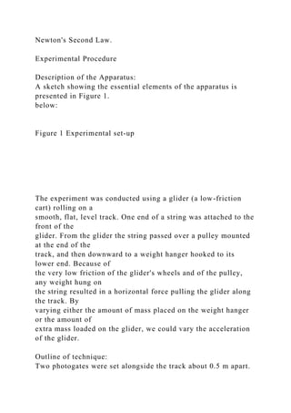
A sketch showing the essential elements of the apparatus is
presented in Figure 1.
below:
Figure 1 Experimental set-up
The experiment was conducted using a glider (a low-friction
cart) rolling on a
smooth, flat, level track. One end of a string was attached to the
front of the
glider. From the glider the string passed over a pulley mounted
at the end of the
track, and then downward to a weight hanger hooked to its
lower end. Because of
the very low friction of the glider's wheels and of the pulley,
any weight hung on
the string resulted in a horizontal force pulling the glider along
the track. By
varying either the amount of mass placed on the weight hanger
or the amount of
extra mass loaded on the glider, we could vary the acceleration
of the glider.
Outline of technique:
Two photogates were set alongside the track about 0.5 m apart.
They were
connected through an interface to a desktop computer. Software
running on the
computer continuously monitored each photogate's light beam.
The cart was
released from rest near one of the photogates. As it was
accelerating it passed
through both photogate beams. It was stopped just before it
reached the pulley.
Whenever a metal strip ("flag") attached to the glider passed
through a light beam,
the beam was interrupted for the amount of time required for the
flag to pass by.
This time interval was measured by the software, which
displayed both the
duration of the interval and the instant of time at the middle of
the interval.
We measured the width of the flag (15 mm) and entered that
value into the
computer. The computer used this value, together with the
measured time
intervals to calculate the average speed of the glider during its
pass through each
photogate.
The procedure has two methods. In both methods the dependent
variables were
the glider's speed when it was at the center of each photogate,
and the time
interval spent between the photogates.
Method 1: The experiment was run four times with four
different values of the
hanging weight, but with the mass of the glider always the
same. In Method 1 the
value of the hanging mass was the independent variable.
Method 2: The experiment was run four more times with the
same hanging weight
each time, but with different loads placed on the glider to vary
its mass. In
Method 2 the mass of the glider was the independent variable.
All masses were measured to the nearest gram using a triple-
beam balance. The
computer displayed, for each run, the average speed of the
glider as it passed
through each photogate beam. These average speeds and the
time interval were
the dependent variables.
Discussion:
Data Summary:
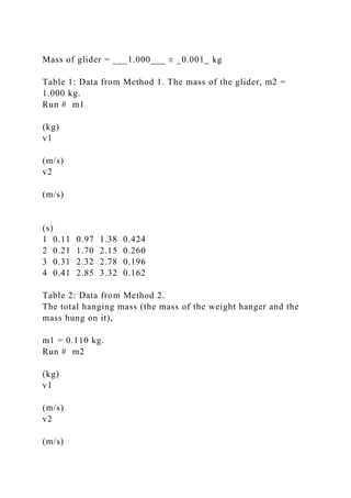
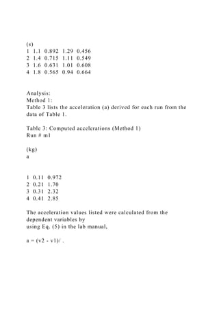
Tables 1 and 2 below present the data obtained by the computer
for each of the
two methods. The velocities listed in columns 3 and 4 and the
time interval
between photogates listed in column 5 were measured by the
computer; those
values were copied from the computer display (see the raw data
in the appendix).
Summary of Measurements
Length of flag = ___0.015_____ ± _0.001_ m
Mass of weight hanger = ___0.010___ ± _0.001_ kg
Mass of glider = ___1.000___ ± _0.001_ kg
Table 1: Data from Method 1. The mass of the glider, m2 =
1.000 kg.
Run # m1
(kg)
v1
(m/s)
v2
(m/s)
(s)
1 0.11 0.97 1.38 0.424
2 0.21 1.70 2.15 0.260
3 0.31 2.32 2.78 0.196
4 0.41 2.85 3.32 0.162
Table 2: Data from Method 2.
The total hanging mass (the mass of the weight hanger and the
mass hung on it),
m1 = 0.110 kg.
Run # m2
(kg)
v1
(m/s)
v2
(m/s)
(s)
1 1.1 0.892 1.29 0.456
2 1.4 0.715 1.11 0.549
3 1.6 0.631 1.01 0.608
4 1.8 0.565 0.94 0.664
Analysis:
Method 1:
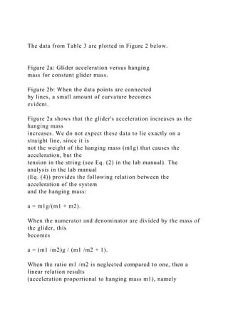
Table 3 lists the acceleration (a) derived for each run from the
data of Table 1.
Table 3: Computed accelerations (Method 1)
Run # m1
(kg)
a
1 0.11 0.972
2 0.21 1.70
3 0.31 2.32
4 0.41 2.85
The acceleration values listed were calculated from the
dependent variables by
using Eq. (5) in the lab manual,
a = (v2 - v1)/ .
The data from Table 3 are plotted in Figure 2 below.
Figure 2a: Glider acceleration versus hanging
mass for constant glider mass.
Figure 2b: When the data points are connected
by lines, a small amount of curvature becomes
evident.
Figure 2a shows that the glider's acceleration increases as the
hanging mass
increases. We do not expect these data to lie exactly on a
straight line, since it is
not the weight of the hanging mass (m1g) that causes the
acceleration, but the
tension in the string (see Eq. (2) in the lab manual). The
analysis in the lab manual
(Eq. (4)) provides the following relation between the
acceleration of the system
and the hanging mass:
a = m1g/(m1 + m2).
When the numerator and denominator are divided by the mass of
the glider, this
becomes
a = (m1 /m2)g / (m1 /m2 + 1).
When the ratio m1 /m2 is neglected compared to one, then a
linear relation results
(acceleration proportional to hanging mass m1), namely
a = m1g / m2.
In this method m1 ranges from 11% to 41% of m2 , so the
approximation m1 /m2
<< 1 is not very accurate here. Even so, the data points in
Figure 2 show, upon
close inspection, only a small departure from a straight line. To
emphasize this the
points have been connected, in Figure 2b, by lines to guide the
eye.
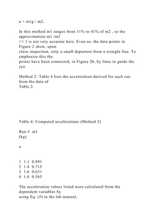
Method 2: Table 4 lists the acceleration derived for each run
from the data of
Table 2.
Table 4: Computed accelerations (Method 2)
Run # m1
(kg)
a
1 1.1 0.891
2 1.4 0.715
3 1.6 0.631
4 1.8 0.565
The acceleration values listed were calculated from the
dependent variables by
using Eq. (5) in the lab manual,
a = (v2 - v1)/ .
The data from Table 4 are plotted in Figure 3 below.
Figure 3: Glider acceleration versus glider mass.
The trend of the data supports the prediction of Newton's
Second Law: for a given
force, acceleration is inversely proportional to mass. To further
check this point,
we plotted the acceleration versus the reciprocal of the mass,
which according to
the second law should be a straight line. That plot is shown in
Figure 4, which
displays a nice linear trend.
Figure 4: Glider acceleration versus reciprocal of glider mass.
Errors:
The systematic errors are associated with uncertainties in the
measurements. The
measured quantities are (1) the flag width, measured to an
accuracy of about 7%,
(2) the masses of the system, measured to accuracies ranging
from about 0.1%, to
1%, and (3) the time intervals (the intervals during which the
flag blocked the
photogate beam). The error in the time interval measurements
depends on the
accuracy of the computer-based timing system, and the errors in
the derived
speeds depend on the accuracy of the computer-based timing
system as well as
the flag length. No information was provided regarding the
accuracy of the timing
system, so we don't know what uncertainties to associate with
the timing
measurement. The data points in Figure 4 were fitted to straight
lines by the
computer using linear least squares software. The program also
calculated the
regression coefficient, R. which is 0.999 for these data points.
A value of 1.00
means perfect agreement between the data and a straight line.
Thus, to a very high
degree of probability our data taken in method 2 are correctly
described by a
linear relation.
Conclusion:
The trends displayed in Figures 2 and 4 generally support the
predictions of
Newton's Second Law. When tested by least squares analysis,
the dependence of
the cart's acceleration on its mass (Figure 4) is in excellent
agreement with the
Second Law: for a given applied force the acceleration is
inversely proportional to
the mass.
Physics Laboratory Report Sample
Physics Laboratory Report Sample    PHY 223 Lab Report .docx

Physics Laboratory Report Sample PHY 223 Lab Report .docx

  • 1.
    Physics Laboratory ReportSample PHY 223 Lab Report Newton's Second Law Your Name: Partner's Full Name(s): Date Performed: Date Due: Date submitted: Lab Section: (number) Instructor: (Name) Introduction We verified Newton's Second Law for one-dimensional motion by timing an accelerated glider moving along a flat track. We varied both the accelerating force and the mass of the glider. We found that for a given force the acceleration of the glider was inversely proportional to the mass of the glider, in agreement with
  • 2.
    Newton's Second Law. ExperimentalProcedure Description of the Apparatus: A sketch showing the essential elements of the apparatus is presented in Figure 1. below: Figure 1 Experimental set-up The experiment was conducted using a glider (a low-friction cart) rolling on a smooth, flat, level track. One end of a string was attached to the front of the glider. From the glider the string passed over a pulley mounted at the end of the track, and then downward to a weight hanger hooked to its lower end. Because of the very low friction of the glider's wheels and of the pulley, any weight hung on the string resulted in a horizontal force pulling the glider along the track. By varying either the amount of mass placed on the weight hanger or the amount of extra mass loaded on the glider, we could vary the acceleration of the glider. Outline of technique: Two photogates were set alongside the track about 0.5 m apart.
  • 3.
    They were connected throughan interface to a desktop computer. Software running on the computer continuously monitored each photogate's light beam. The cart was released from rest near one of the photogates. As it was accelerating it passed through both photogate beams. It was stopped just before it reached the pulley. Whenever a metal strip ("flag") attached to the glider passed through a light beam, the beam was interrupted for the amount of time required for the flag to pass by. This time interval was measured by the software, which displayed both the duration of the interval and the instant of time at the middle of the interval. We measured the width of the flag (15 mm) and entered that value into the computer. The computer used this value, together with the measured time intervals to calculate the average speed of the glider during its pass through each photogate. The procedure has two methods. In both methods the dependent variables were the glider's speed when it was at the center of each photogate, and the time interval spent between the photogates. Method 1: The experiment was run four times with four different values of the hanging weight, but with the mass of the glider always the same. In Method 1 the
  • 4.
    value of thehanging mass was the independent variable. Method 2: The experiment was run four more times with the same hanging weight each time, but with different loads placed on the glider to vary its mass. In Method 2 the mass of the glider was the independent variable. All masses were measured to the nearest gram using a triple- beam balance. The computer displayed, for each run, the average speed of the glider as it passed through each photogate beam. These average speeds and the time interval were the dependent variables. Discussion: Data Summary: Tables 1 and 2 below present the data obtained by the computer for each of the two methods. The velocities listed in columns 3 and 4 and the time interval between photogates listed in column 5 were measured by the computer; those values were copied from the computer display (see the raw data in the appendix). Summary of Measurements Length of flag = ___0.015_____ ± _0.001_ m Mass of weight hanger = ___0.010___ ± _0.001_ kg
  • 5.
    Mass of glider= ___1.000___ ± _0.001_ kg Table 1: Data from Method 1. The mass of the glider, m2 = 1.000 kg. Run # m1 (kg) v1 (m/s) v2 (m/s) (s) 1 0.11 0.97 1.38 0.424 2 0.21 1.70 2.15 0.260 3 0.31 2.32 2.78 0.196 4 0.41 2.85 3.32 0.162 Table 2: Data from Method 2. The total hanging mass (the mass of the weight hanger and the mass hung on it), m1 = 0.110 kg. Run # m2 (kg) v1 (m/s) v2 (m/s)
  • 6.
    (s) 1 1.1 0.8921.29 0.456 2 1.4 0.715 1.11 0.549 3 1.6 0.631 1.01 0.608 4 1.8 0.565 0.94 0.664 Analysis: Method 1: Table 3 lists the acceleration (a) derived for each run from the data of Table 1. Table 3: Computed accelerations (Method 1) Run # m1 (kg) a 1 0.11 0.972 2 0.21 1.70 3 0.31 2.32 4 0.41 2.85 The acceleration values listed were calculated from the dependent variables by using Eq. (5) in the lab manual, a = (v2 - v1)/ .
  • 7.
    The data fromTable 3 are plotted in Figure 2 below. Figure 2a: Glider acceleration versus hanging mass for constant glider mass. Figure 2b: When the data points are connected by lines, a small amount of curvature becomes evident. Figure 2a shows that the glider's acceleration increases as the hanging mass increases. We do not expect these data to lie exactly on a straight line, since it is not the weight of the hanging mass (m1g) that causes the acceleration, but the tension in the string (see Eq. (2) in the lab manual). The analysis in the lab manual (Eq. (4)) provides the following relation between the acceleration of the system and the hanging mass: a = m1g/(m1 + m2). When the numerator and denominator are divided by the mass of the glider, this becomes a = (m1 /m2)g / (m1 /m2 + 1). When the ratio m1 /m2 is neglected compared to one, then a linear relation results (acceleration proportional to hanging mass m1), namely
  • 8.
    a = m1g/ m2. In this method m1 ranges from 11% to 41% of m2 , so the approximation m1 /m2 << 1 is not very accurate here. Even so, the data points in Figure 2 show, upon close inspection, only a small departure from a straight line. To emphasize this the points have been connected, in Figure 2b, by lines to guide the eye. Method 2: Table 4 lists the acceleration derived for each run from the data of Table 2. Table 4: Computed accelerations (Method 2) Run # m1 (kg) a 1 1.1 0.891 2 1.4 0.715 3 1.6 0.631 4 1.8 0.565 The acceleration values listed were calculated from the dependent variables by using Eq. (5) in the lab manual,
  • 9.
    a = (v2- v1)/ . The data from Table 4 are plotted in Figure 3 below. Figure 3: Glider acceleration versus glider mass. The trend of the data supports the prediction of Newton's Second Law: for a given force, acceleration is inversely proportional to mass. To further check this point, we plotted the acceleration versus the reciprocal of the mass, which according to the second law should be a straight line. That plot is shown in Figure 4, which displays a nice linear trend. Figure 4: Glider acceleration versus reciprocal of glider mass. Errors: The systematic errors are associated with uncertainties in the measurements. The measured quantities are (1) the flag width, measured to an accuracy of about 7%, (2) the masses of the system, measured to accuracies ranging from about 0.1%, to 1%, and (3) the time intervals (the intervals during which the flag blocked the photogate beam). The error in the time interval measurements depends on the accuracy of the computer-based timing system, and the errors in the derived
  • 10.
    speeds depend onthe accuracy of the computer-based timing system as well as the flag length. No information was provided regarding the accuracy of the timing system, so we don't know what uncertainties to associate with the timing measurement. The data points in Figure 4 were fitted to straight lines by the computer using linear least squares software. The program also calculated the regression coefficient, R. which is 0.999 for these data points. A value of 1.00 means perfect agreement between the data and a straight line. Thus, to a very high degree of probability our data taken in method 2 are correctly described by a linear relation. Conclusion: The trends displayed in Figures 2 and 4 generally support the predictions of Newton's Second Law. When tested by least squares analysis, the dependence of the cart's acceleration on its mass (Figure 4) is in excellent agreement with the Second Law: for a given applied force the acceleration is inversely proportional to the mass. Physics Laboratory Report Sample