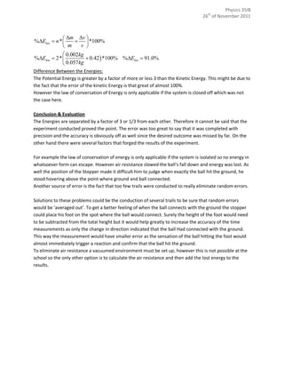
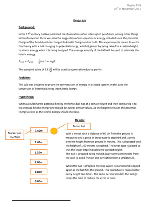
This physics lab experiment was designed to verify Galileo's theory of conservation of energy by measuring the potential and kinetic energy of a falling tennis ball. The ball was dropped from various heights and its time of fall was recorded. Calculations showed the potential energy was about 3 times greater than the kinetic energy, failing to prove conservation of energy. Sources of error included air resistance, imprecise timing of when the ball hit the ground, and too few trials. Improving the experiment could help address these issues and better test the hypothesis.

1. Physics 35IB
26th of November 2011
Design Lab
Background:
In the 17th century Galileo published his observations of an interrupted pendulum, among other things.
In his observation there was also the suggestion of conservation of energy included since the potential
Energy of the Pendulum bob changed to kinetic Energy and so forth. This experiment is meant to verify
this theory with a ball changing its potential energy, which it gained by being raised to a certain height,
to kinetic energy when it is being dropped. The average velocity of the ball will be used to calculate the
kinetic energy.
The accepted value of 9.81 will be used as acceleration due to gravity.
Problem:
This Lab was designed to prove the conversation of energy in a closed system. In this case the
conversion of Potential Energy into Kinetic Energy.
Hypothesis:
When calculating the potential Energy the tennis ball has at a certain height and then comparing it to
the average kinetic energy one should get rather similar values. As the height increases the potential
Energy as well as the kinetic Energy should increase.
Design:
Tennis ball
1.60m
Markers on With a meter stick a distance of 60 cm from the ground is
the Wall measured and a piece of crepe tape is attached and labeled
1.40m with the height from the ground in meters. This is repeated until
the height of 1.60 meters is reached. The crept tape is placed so
that the lower edge indicates the wanted height.
1.20m The Ball is dropped being moved away some centimeters from
the wall to avoid friction and derivation from a straight fall.
1.00m
When the ball is dropped the stop watch is started and stopped
again as the ball hits the ground. This procedure is repeated for
0.80m
every height two times. The same person who lets the ball go
stops the time to reduce the error in time.
0.60m

2. Physics 35IB
26th of November 2011
Materials:
 Crepe tape
 Stop watch
 Tennis ball
 Meter Stick
Variables:
Independent: The height of each trail – The ball was moved after being dropped upwards by 0.20 cm the
same markers were used every time.
Corresponding: The (average) velocity – the same ball was used in all of the trails and the distance
between wall and ball was approximately always the same. The ball was moved into the same height
twice to prevent/minimize random errors.
Controlled:
1. The Tennis Ball – The same ball was used in all trails and it was not modified in any kind of way to
ensure that the aerodynamic properties and the weight stayed the same and did not forge the stopped
time.
2. The stopper(person) - The same person was used to take the time in each trail otherwise the
fluctuations in reaction time would have made a determination of the error in the stopped time difficult.
3. The markers – The height the ball was dropped was always determined by the same marker who
stayed in the same place throughout the whole conduction of the experiment. A change would have
resulted in a derivation in height from the former trial.
4. The distance between the wall and ball - In every trial the person who dropped the ball moved it
away from the wall roughly the same distance as in all the other trails so to ensure that no friction
between the ball and the wall occurred which would have caused a slow-down.
5. The environment – The trail was conducted in the same environment/place. This was done to ensure
that factors like wind, pressure or temperature did not change greatly. The experiment was conducted
inside to prevent sudden gushes of wind from influencing the records.
Procedures:
1. Take the Meter Stick and place it straight as possible against the wall.
2. Measure a distance of 0.60 m from the ground.
3. Place a piece of crepe tape so the lower edge matches up exactly with the desired value. Record
the value on the marker in meter.
4. Raise the Meter Stick and measure 0.20 m from the lower edge of the marker.
5. Repeat Steps 3 and 4 until you reach 1.60 m from the ground.
6. Start at the top marker (1.60m).
7. Place ball at the lower edge of the marker and move it away from the wall.

3. Physics 35IB
26th of November 2011
8. Drop it and at the same time start the Stop Watch.
9. When the ball hits the floor stop the time and record it. Move the ball down to the next marker.
10. Repeat Steps 7 to 9 until two full rounds of trails are completed.
Measurements:
Mass of the Tennis Ball: 0.05697 ± 0.002kg
Accepted Value for Acceleration due to Gravity: 9.81 ms-1
Height in m Time in s ± 0.15s Average Time in
± 0.002m Trail 1 Trail 2 s ± 0.17s
1.60 0.60 0.58 0.59
1.40 0.57 0.54 0.56
1.20 0.45 0.47 0.46
1.00 0.40 0.42 0.41
0.80 0.30 0.37 0.34
0.60 0.24 0.31 0.28
Table 1.0. – Raw Data. (Height, Time of both trails and averaged Time)
The Average Time was calculated with according to following formula:
t1  t2
time( x)ave 
2
0.24s  0.31s 0.55s
time(0.60) ave    0.275s
2 2
To attain the average velocity to compare Epot and Ekin later on in the experiment the height h will be
divided by the averaged time t.
Height in m Average
± 0.002m Velocity in ms-1
± 42%
1.60 2.71
1.40 2.50
1.20 2.61
1.00 2.44
0.80 2.35
0.60 2.14
Table 1.1 – Progressed Data. (Height and average velocity of the ball)

4. Physics 35IB
26th of November 2011
h
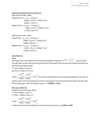
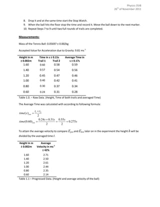
The Velocity was calculated using the formula of vave  as an example:
s
0.60m m
vave   2.14
0.28s s
Uncertainties:
The Uncertainty of the raw time Data was set at 0.15 s which is equivalent to the reaction time of the
person who stopped the time. As the time was stopped when the ball hit the ground an average
reaction time of 0.15 seconds would need to be added or subtracted. The error of the height of 0.002m
(0.2cm) does not equal the maximum degree of uncertainty of 0.05cm since a perfect determination of
the height was made impossible because of bad shape the used ruler was in.
The uncertainty of average time was attained through the arithmetic mean calculations.
[ greatest value]  [mean]  ...
Whatever value was the greater residual will be used as uncertainty.
[ smallest value]  [mean]  ...
0.59s  0.44s  0.15s
As the minus in front can be neglected the value of 0.17 seconds is the greater
0.28s  0.44s  0.17 s
of both of them. Therefore the 0.17 s was used as error when dealing with the average time.
When determining the error of the average velocity one needs to follow through with following steps.
First the Formula of Error Propagation needs to be determined. The average Velocity is attained through
Division of two values with corresponding errors; The formula for Division:
 h t  m  0.002m 0.17s  v  1.33 m
vave  vave *   ave  an example for this: vave  2.14 *    ave
 h t  s  0.6m 0.28s  s
To make calculations later on easier the percent Uncertainty is needed.
m
1.33
vave s *100%
%vave  *100% ; %vave  %vave  0.62%
vave m
2.14
s
Afterwards all of the calculated values for the average velocity percent error are being averaged to a
value of 42%.
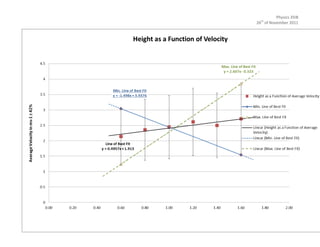
Only on the axis with the greater percentage error Error bars are used to indicate the rage of the value.
The average percentage uncertainty of height is 0.20% and the uncertainty of velocity is 42%.
Y-error bars will be used.

5. Physics 35IB
26th of November 2011
Maximum and Minimum Line of Best Fit:
Data Points for Max. LofBF:
Lowest Point = xmin, ymin - error(ymin)
0.60m, 2.14 ms-1 – 42%2.14 ms-1
(0.60m, 1.24 ms-1)
Highest Point = xmax, ymax + error(ymax)
1.60m, 2.71 ms-1+ 42%x2.71 ms-1
(1.60m, 3.85 ms-1)
Data Points for Min. LofBF:
Lowest Point: xmin, ymin + error(ymin)
0.60m, 2.14 ms-1 + 42%2.14 ms-1
(0.60m, 3.04 ms-1)
Highest Point = xmax, ymax - error(ymax)
1.60m, 2.71 ms-1- 42%x2.71 ms-1
(1.60m, 1.54 ms-1)
Line of Best Fit:
Slope: y2 - y1
The slope of the Line of Best fit can be calculated using the equation of slope = x2, - x1 ,but the points
must be taken so that they cover the greater part of the graph in this case the first and the last point are
the most reasonable choices:
1st Point: (0.60m, 2.14 ms-1)
Last Point: (1.60m, 2.71 ms-1)
m m
2.71  2.14
slope  s s  0.57 1 This comes relatively close to the Equation displayed on the chart. A
1.60m  0.60m s
perfect match cannot be expected since the excel program uses finer techniques to determine the slope
of the linear graph. The final Equation used is y = 0.4957x + 1.913
Max. Line of Best Fit:
Using the same techniques above;
1st Point: (0.60m, 1.24 ms-1)
2nd Point: (1.60m, 3.85 ms-1)
m m
3.85  1.24
slope  s s  2.61 1
1.60m  0.60m s
As before with the same explanation the equation on the chart is y = 2.607x - 0.323

6. Physics 35IB
26th of November 2011
Min. Line of Best Fit:
Using the same techniques as above;
1st Point: (0.60m, 3.04 ms-1)
2nd Point: (1.60m, 1.54 ms-1)
m m
1.54  3.04
slope  s s  1.50 1
1.60m  0.60m s
The Equation on the start states the more accurate value of y = -1.498x + 3.9376
Uncertainty for slope calculations:
slope  Slope of Max. LofBF  Slope of Min. LofBF
1 1 1
slope  2.61  (1.50 ) slope  4.11
s s s
Conservation of Energy
Epot=Ekin
1
hmg  mv 2
2
m 1
E pot  h *0.057kg *9.81 E pot  0.057kg * * v 2
s2 2
Epot Ekin
0.89 0.21
0.78 0.18
0.67 0.19
0.56 0.17
0.45 0.16
0.34 0.13
2.0 Table – Comparison of the two Energies.
Uncertainties of Energy
 m h 
%E pot     *100%
 m h 
 0.002kg 0.002m 
%E pot     *100% %E pot  3.6%
 0.057kg 1.60m 

7. Physics 35IB
26th of November 2011
 m v 
%Ekin  n *    *100%
 m v 
 0.002kg
%Ekin  2*   0.42  *100% %Ekin  91.0%
 0.057kg
Difference Between the Energies:
The Potential Energy is greater by a factor of more or less 3 than the Kinetic Energy. This might be due to
the fact that the error of the kinetic Energy is that great of almost 100%.
However the law of conversation of Energy is only applicable if the system is closed off which was not
the case here.
Conclusion & Evaluation
The Energies are separated by a factor of 3 or 1/3 from each other. Therefore it cannot be said that the
experiment conducted proved the point. The error was too great to say that it was completed with
precision and the accuracy is obviously off as well since the desired outcome was missed by far. On the
other hand there were several factors that forged the results of the experiment.
For example the law of conservation of energy is only applicable if the system is isolated so no energy in
whatsoever form can escape. However air resistance slowed the ball’s fall down and energy was lost. As
well the position of the Stopper made it difficult him to judge when exactly the ball hit the ground, he
stood hovering above the point where ground and ball connected.
Another source of error is the fact that too few trails were conducted to really eliminate random errors.
Solutions to these problems could be the conduction of several trails to be sure that random errors
would be ‘averaged out’. To get a better feeling of when the ball connects with the ground the stopper
could place his foot on the spot where the ball would connect. Surely the height of the foot would need
to be subtracted from the total height but it would help greatly to increase the accuracy of the time
measurements as only the change in direction indicated that the ball Had connected with the ground.
This way the measurement would have smaller error as the sensation of the ball hitting the foot would
almost immediately trigger a reaction and confirm that the ball hit the ground.
To eliminate air resistance a vacuumed environment must be set up, however this is not possible at the
school so the only other option is to calculate the air resistance and then add the lost energy to the
results.

8. Physics 35IB
26th of November 2011

9. Physics 35IB
26th of November 2011