1 Computer Assignment 3 --- Hypothesis tests about means Statistics, Fall 2014, Singleton Microsoft Excel has two data analysis tools that are very useful for hypothesis testing about population means as done in the textbook, chapters 9 and 10. These are 1) t-Test: Two-Sample Assuming Equal Variances 2) t-Test: Two-Sample Assuming Unequal Variances These tools utilize the two sets of equations in Chapter 10 of the text, namely (1) on page 368 assuming equal variances, and (2) on page 369 assuming unequal variances. Number 1 tool (equal variances) is strictly for Chapter 10 problems with two samples, each from its own population, and you are attempting to compare the two population means, and by hypothesis tests involving . Number 2 tool (unequal variances) can be used for Chapter 9 or Chapter 10 problems. In previous online classes taught by Dr Revere, she had students use a combination of various Excel functions to do Chapter 9 t-tests about . It seems to me that using the unequal-variance tool is easier. On page 353 of the text there is an almost-correct description of how to use the Chapter- 10-style t-test for Chapter 9. In using a Chapter 10 test for Chapter 9, instead of comparing 2 sets of data, the second set of data is replaced with a fixed hypothesized value (which has zero variation). Steps are (for Ch 9 problems) ---Enter a column of your n values of experimental data to be tested. ---Enter another column of at least two of the hypothesized value being tested against (if the null hypothesis has =1.84 or ≤1.84 or ≥1.84 enter at a column of at least two 1.84’s (contrary to what the book says, you do not have to use n 1.84’s). ---With menus open the “t-Test: Two-Sample Assuming Unequal Variances” analysis tool. ---Select the “Variable 1 Range” to contain the experimental data. ---Select the “Variable 2 Range” to contain at least two identical values of the number in the null hypothesis (see the example below which has 1.84). (The book says enter n of them.) 2 ---Enter 0 for the “Hypothesized Mean Difference” ---Set the “Labels” checkbox using the rules you obeyed for data in Computer Assignment 1. In many of the problems the data are set up NOT to use labels. ---Make sure you set “Alpha” to your specified value. Also typing it on the worksheet is helpful as a reminder. ---The output is going to be compact and I suggest that you set “Output Range” to a cell near the data. ---Click OK When you do a Chapter 9 problem this way you are comparing your sample data, which has a variance that is calculated by Excel, with your hypothesized value, which has a variance of zero since you entered 2 or more identical values for it. Your “Hypothesized Mean Difference” must always be zero. Of course this requires the “t-Test: Two-Sample Assuming Unequal Variances” tool. Why does this work? If s22 and  are both zero in the equat ...

1. 1
Computer Assignment 3 --- Hypothesis tests about means
Statistics, Fall 2014, Singleton
Microsoft Excel has two data analysis tools that are very useful
for hypothesis testing about
population means as done in the textbook, chapters 9 and 10.
These are
1) t-Test: Two-Sample Assuming Equal Variances
2) t-Test: Two-Sample Assuming Unequal Variances
These tools utilize the two sets of equations in Chapter 10 of
the text, namely (1) on page 368
assuming equal variances, and (2) on page 369 assuming
unequal variances.
Number 1 tool (equal variances) is strictly for Chapter 10
problems with two samples, each
from its own population, and you are attempting to compare the
two population means,
Number 2 tool (unequal variances) can be used for Chapter 9
or Chapter 10 problems. In
previous online classes taught by Dr Revere, she had students
use a combination of various Excel
functions to do Chapter 9 t-
using the unequal-variance tool is
easier. On page 353 of the text there is an almost-correct

2. description of how to use the Chapter-
10-style t-test for Chapter 9. In using a Chapter 10 test for
Chapter 9, instead of comparing 2
sets of data, the second set of data is replaced with a fixed
hypothesized value (which has zero
variation).
Steps are (for Ch 9 problems)
---Enter a column of your n values of experimental data to be
tested.
---Enter another column of at least two of the hypothesized
value being tested against (if the null
of at least two 1.84’s (contrary to
what the book says, you do not have to use n 1.84’s).
---With menus open the “t-Test: Two-Sample Assuming
Unequal Variances” analysis tool.
---Select the “Variable 1 Range” to contain the experimental
data.
---Select the “Variable 2 Range” to contain at least two
identical values of the number in the
null hypothesis (see the example below which has 1.84). (The
book says enter n of them.)
2
---Enter 0 for the “Hypothesized Mean Difference”
---Set the “Labels” checkbox using the rules you obeyed for

3. data in Computer Assignment 1.
In many of the problems the data are set up NOT to use labels.
---Make sure you set “Alpha” to your specified value. Also
typing it on the worksheet is helpful
as a reminder.
---The output is going to be compact and I suggest that you set
“Output Range” to a cell near the
data.
---Click OK
When you do a Chapter 9 problem this way you are comparing
your sample data, which has a
variance that is calculated by Excel, with your hypothesized
value, which has a variance of zero
since you entered 2 or more identical values for it. Your
“Hypothesized Mean Difference”
must always be zero. Of course this requires the “t-Test: Two-
Sample Assuming Unequal
Variances” tool.
Why does this work?
variances, page 369, these equations
reduce to the equations in Chapter 9 for one sample, “t-Test for
3
For the degrees of freedom

4. 4
To do a Chapter 10 problem, you instead use the two samples
of data which need to be
compared. The “Hypothesized Mean Difference” is not
necessarily zero (but frequently is), and
you may want to use the “t-Test: Two-Sample Assuming Equal
Variances” tool for Chapter 10
since the problems usually call for it, although relaxing the
equal variance assumption is
obviously more general.
To do a problem in this assignment without Excel (with a
calculator), you have to compute the
requisite sample mean(s) and standard deviation(s) and then
compute the test t with the correct
formula, and finally use the same logic which you need for this
assignment for choices of
number of tails, critical value(s), etc. I am hoping this
assignment gets you to learn this logic;
you should also get some practice in computing by calculator in
other homework not turned in.
An example for Chapter 9:
9.17.
A hole-punch machine is set to punch a hole 1.84 centimeters in
diameter in a strip of
sheet metal in a manufacturing process. The strip of metal is
then creased and sent on to the next
phase of production, where a metal rod is slipped through the
hole. It is important that the hole
be punched to the specified diameter of 1.84 cm. To test
punching accuracy, technicians have

5. randomly sampled 12 punched holes and measured the
diameters. The data (in centimeters)
follow. Use an alpha of .10 to determine whether the holes are
being punched an average of 1.84
centimeters. Assume the punched holes are normally distributed
in the population.
Because the question asks whether the mean is equal or not, one
has to consider that it could be
unequal in either the + or – directions, so the problem is 2-
tailed. The hypotheses must be
5
Data Hypothesis Output
1.81 1.84 t-Test: Two-Sample Assuming Unequal Variances
1.85 1.84
1.84 Variable 1 Variable 2
1.89 Mean 1.850833333 1.84
1.82 Variance 0.000553788 0
1.86 Observations 12 2
1.86 Hypothesized Mean Difference 0
1.87 df 11
1.88 t Stat 1.594707389 =test t result
1.83 P(T<=t) one-tail 0.069542202
1.85 t Critical one-tail 1.363430318
1.85 P(T<=t) two-tail 0.139084405 =p-value result
t Critical two-tail 1.795884819 =+/-tc for Alpha=0.1 two-tailed

6. The toolkit form for this is
Summary of results
a) Decision is: Fail to reject H0
b) Test t = 1.59471
c) p-value for this test is = 0.139
d) Critical t value(s) is/are +/- 1.79588 based on
alpha=0.1
Since the problem calls for a two-tailed test, we should not use
the one-tail results, but if it were
restated as a one-tail problem, then the one-tail and not the two-
tail results would apply, although
6
the computer calculations would be the same. For the two-
tailed test, since the p-value is about
0.14, larger than 0.1, the diameter is not significantly different
from 1.84 at the 0.1 level, but
for the one-tailed test it is significantly greater than 1.84 at the
0.1 level since the one-tailed p-
value is about 0.07, less than 0.1.
To do this assignment you have to tell whether it is 1-tail or 2-
tail by reading the problem
statement. Numbers for both cases are computed, but I require
you to tell me which apply!
Also note that the computer always gives the critical t as
positive, but, depending on the

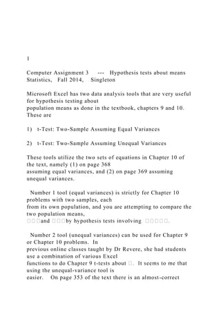
7. alternate 1-tail hypothesis, the critical t might really have to be
stated as negative (same
thing happens when using the t-table in the textbook). If the
test t is negative, the 1-tailed
critical t is negative. (Neglecting the trivial case where you are
trying to show the test value is
negative, but it by random chance turns out to be positive so
you automatically fail to reject H0 -
----- book problems never do this.)
For 2-tailed hypotheses there are two (+ and –) critical values.
The only disappointment I have with Excel is that the value of
alpha that you specify determines
the “t Critical” output results, but alpha is nowhere restated in
the output. Make sure you specify
the correct alpha, or your critical value results will be in error.
In modern research practice alpha is seldom stated and
hypotheses usually are stated less
formally than in our text. The result of the test is usually just
stated by giving the p-value, which
is recognized as the level of significance of the test. However,
our text does not equip us to get
p-values for t-tests as there would have to be a much larger set
of tables for us to look them up.
The Excel analysis tools allow us to do this.
Graphical presentation of the results for 9.17:
Ideally scale drawings of the t-distribution could be presented,
but in practice we just make
approximate diagrams. If you are turning in this assignment in
the classroom, a quick hand
sketch is sufficient. For those of you who are turning this in by
internet, images of distributions

8. with tails are present in the data files. You can select and copy
the appropriate image and type
numeric values underneath.
7
Critical t’s
tc=-1.796 tc=+1.796
p-value diagram
-1.595 left tail test t= 1.595
In this case the right-hand (positive) tail is at the (positive) test
t value, and since it is a 2-tail problem
you have to indicate the 2nd tail on the left.
Your Task:
There are 8 hypothesis test problems to work out, with 7 of
them directly from the book, and I
ask you to do two of them two ways, make 10 problems
altogether. You need to use either the
data analysis tool “t-Test: Two-Sample Assuming Unequal
Variances” or “t-Test: Two-Sample
Assuming Equal Variances”, depending on the requirements of
the problem and I am
conveniently providing files with the data already set up. First
of all, you have to
8

9. decide from the wording of the problem, whether there are one
or two tails.
The computer does not tell you whether you have a one-tailed or
two-tailed test,
and a major source of student error has been in picking the
wrong case. The
problems do not all have 2 tails like the example.
Turn in the Excel files with answers as an email attachment.
The assignment is divided into 2
parts, one for Ch 9 and one for Ch 10, with different due dates.
Also, you need to report
summary answers as asked in each problem statement. The
computer summaries can be done
by adding a summary table next to the computer output.
Copying and pasting text from this file
to the spreadsheet can make things easier. For some of the
problems I ask you to copy, paste,
and label the diagrams I give you in the Excel file (see the
example above).
Problem 1
9.15 The following data were gathered from a random sample
of 11 items.
1200 1175 1080 1275 1201 1387
1090 1280 1400 1287 1225
Use these data and a 5% level of significance to test the
following hypotheses, assuming
that the data come from a normally distributed population.
Use the appropriate method in an Excel spreadsheet. Then
summarize your results by adding the

10. following to your spreadsheet (I found I could copy and paste
items into the spreadsheet rather than
retyping them).
a) Decision is:
b) Test t =
c) p-value for this test is =
d) Critical t value(s) is/are
e) Sketch or copy and paste a little distribution
diagram and label the critical t value(s)
f) Sketch or copy and paste a little distribution diagram
and label the tail boundaries bounding
the p-value tail(s).
9
Problem 2
9.16. The following data (in pounds), which were selected
randomly from a normally distributed
population of values, represent measurements of a machine part
that is supposed to weigh,
on average, 8.3 pounds.
8.1 8.4 8.3 8.2 8.5 8.6 8.4 8.3 8.4 8.2
8.8 8.2 8.2 8.3 8.1 8.3 8.4 8.5 8.5 8.7
Use these data and α = .01 to test the hypothesis that the parts

11. average 8.3 pounds.
Use the appropriate method in an Excel spreadsheet. Then
summarize your results by adding the
following to your spreadsheet .
a) Decision is:
b) Test t =
c) p-value for this test is =
d) Critical t value(s) is/are
e) Sketch or copy and paste a little distribution
diagram and label the critical t value(s)
f) Sketch or copy and paste a little distribution diagram
and label the tail boundaries bounding
the p-value tail(s).
10
Problem 3
9.18 Suppose a study reports that the average price for a gallon
of self-serve regular unleaded
gasoline is $3.76. You believe that the figure is higher in your
area of the country. You
decide to test this claim for your part of the United States by
randomly calling gasoline
stations. Your random survey of 25 stations produces the
following prices.

12. $3.87 $3.89 $3.76 $3.80 $3.97
3.80 3.83 3.79 3.80 3.84
3.76 3.67 3.87 3.69 3.95
3.75 3.83 3.74 3.65 3.95
3.81 3.74 3.74 3.67 3.70
Assume gasoline prices for a region are normally distributed.
Do the data you obtained
provide enough evidence to reject the claim? Use a 1% level of
significance.
a) Decision is:
b) Test t =
c) p-value for this test is =
d) Critical t value(s) is/are
e) Copy and paste a little distribution diagram and
label the critical t value(s)
f) Copy and paste a little distribution diagram and label
the tail boundaries bounding the p-value
tail(s).
11
Problem 4
9.64 Downtime in manufacturing is costly and can result in late
deliveries, backlogs, failure to
meet orders, and even loss of market share. Suppose a
manufacturing plant has been

13. averaging 23 minutes of downtime per day for the past several
years, but during the past
year, there has been a significant effort by both management
and production workers to
reduce downtime. In an effort to determine if downtime has
been significantly reduced,
company productivity researchers have randomly sampled 31
days over the past several
months from company records and have recorded the daily
downtimes shown below in
minutes. Use these data and an alpha of .01 to test to determine
if downtime has been
significantly reduced. Assume that daily downtimes are
normally distributed in the
population.
19 22 17 19 32 24 16 18 27 17
24 19 23 27 28 19 17 18 26 22
19 15 18 25 23 19 26 21 16 21
24
a) Decision is:
b) Test t =
c) p-value for this test is =
d) Critical t value(s) is/are
12
Problem 5 (beginning assignment 3B)

14. 10.16 According to an Experiential Education Survey published
at JobWeb.com, the average
hourly wage of a college student working as a co-op is $15.64
an hour and the average
hourly wage of an intern is $15.44. Assume that such wages are
normally distributed in
the population and that the population variances are equal.
Suppose these figures were
actually obtained from the data below.
Co-op
Students Interns
$15.34 $15.10
14.75 14.45
15.88 16.21
16.92 14.91
16.84 13.80
17.37 16.02
14.05 16.25
15.41 15.89
16.74 13.99
14.55 16.48
15.25 15.75
14.64 16.42
Use these data and to test to determine if there is a significant
difference in the mean hourly wage of a college co-op student
and the
mean hourly wage of an intern.
a) Decision is:
b) Test t =
c) p-value for this test is =

15. d) Critical t value(s) is/are
13
Problem 6
10.20. Some studies have shown that in the United States, men
spend more than women buying
gifts and cards on Valentine's Day. Suppose a researcher wants
to test this hypothesis by
randomly sampling nine men and 10 women with comparable
demographic
characteristics from various large cities across the United States
to be in a study. Each
study participant is asked to keep a log beginning one month
before Valentine's Day and
record all purchases made for Valentine's Day during that one-
month period. The
resulting data are shown below. Use these data and a 1% level
of significance to test to
determine if, on average, men actually do spend significantly
more than women on
Valentine's Day. Assume that such spending is normally
distributed in the population and
that the population variances are equal.
Men Women
$107.48 $125.98
143.61 45.53
90.19 56.35

16. 125.53 80.62
70.79 46.37
83.00 44.34
129.63 75.21
154.22 68.48
93.80 85.84
126.11
a) Decision is:
b) Test t =
c) p-value for this test is =
d) Critical t value(s) is/are
14
e) Copy and paste a little distribution diagram and label the
critical t value(s)
f) Copy and paste a little distribution diagram and label
the tail boundaries bounding the p-value
tails.
Problem 7
Also repeat the calculation using the Excel routine for NON-

17. EQUAL population variances to
show any differences from above.
a) Decision is:
b) Test t =
c) p-value for this test is =
d) Critical t value(s) is/are
Since the non-equal case is more general, these answers should
be preferred to those for problem 6, but
the equal-variances case is accepted as sufficiently accurate for
nearly all t-tests mentioned in Chapter
10. The equal-variances case always has an integer and easy-to-
calculate degrees of freedom.
15
Problem 8
10.64 As the prices of heating oil and natural gas increase,
consumers become more careful
about heating their homes. Researchers want to know how warm
homeowners keep their
houses in January and how the results from Wisconsin and
Tennessee compare. The
researchers randomly call 23 Wisconsin households between 7
P.M. and 9 P.M. on January
15 and ask the respondent how warm the house is according to
the thermostat. The
researchers then call 19 households in Tennessee the same night
and ask the same

18. question. The results follow.
Wisconsin Tennessee
71 71 65 68 73 75 74 71
70 61 67 69 74 73 74 70
75 68 71 73 72 71 69 72
74 68 67 69 74 73 70 72
69 72 67 72 69 70 67
70 73 72
For , is the average temperature of a house in Tennessee
significantly higher than
that of a house in Wisconsin on the evening of January 15?
Assume the population
variances are equal and the house temperatures are normally
distributed in each
population.
a) Decision is:
b) Test t =
c) p-value for this test is =
d) Critical t value(s) is/are
e) Copy and paste a little distribution diagram and
label the critical t value(s)
f) Copy and paste a little distribution diagram and label

19. the tail boundaries bounding the p-value
tails.
16
Problem 9
The sample data below were artificially generated by sampling
with the Excel random number generator
in normal distribution mode. Variable X1 was deliberately
made to have a much larger population
variance than variable X2, whereas in virtually all of the
textbook examples and problems, the
assumption of equal population variances is made (“pooled
variance”).
Test whether the population mean of X1 larger than that of X2.
When you compute the sample means
you will see that the sample mean for X1 is a little larger than
for X2, but is this significant at the 0.05
level? What is its level of significance (p-value)?
Use the Excel tool for unequal variance.
81.89291652 68.32479
66.30485945 59.64873
58.55150807 61.55066
79.38375706 58.91033
69.94111022 55.63936
85.53003131 64.79779
99.00587788 60.14308
64.89543825 53.81751
44.01473593 59.75551

20. 59.8413
66.57747
63.9125
a) Decision is:
b) Test t =
c) p-value for this test is =
d) Critical t value(s) is/are
Problem 10
Repeat problem 9 with the Excel tool for equal (“pooled”)
variance to see how different its answers are.
Of course, answers for the pooled method are suspect in this
case.
a) Decision is:
b) Test t =
c) p-value for this test is =
d) Critical t value(s) is/are
example - Table 1DataHypothesisOutput1.811.84t-Test: Two-
Sample Assuming Unequal Variances1.851.841.84Variable
1Variable
21.89Mean1.85083333331.841.82Variance0.000553787901.86O
bservations1221.86Hypothesized Mean
Difference01.87df111.88t Stat1.5947073886=test t1.83P(T<=t)
one-tail0.06954220231.85t Critical one-

21. tail1.3634303181.85P(T<=t) two-tail0.1390844046=p-valuet
Critical two-tail1.7958848187=+/-tc for Alpha=0.1 two-tailed
test
9.15 - Table
112001090117512801080140012751287120112251387
9.16 - Table 19.16.Weight of machine part,
lb8.18.48.38.28.58.68.48.38.48.28.88.28.28.38.18.38.48.58.58.7
9.18 - Table 19.18 ---price
$/gallon3.873.83.763.753.813.893.833.673.833.743.763.793.873
.743.743.83.83.693.653.673.973.843.953.953.7
9.64 - Table
11922171932241618271724192327281917182622191518252319
2621162124
Distribution templates - Table 1-tail2-tail1-tail