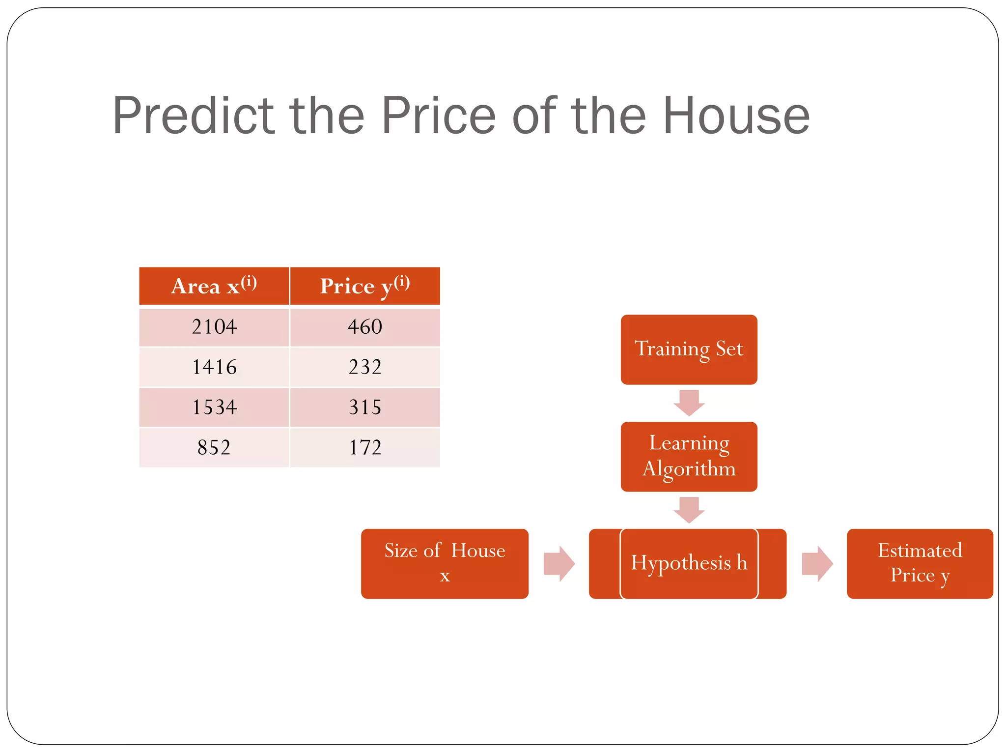
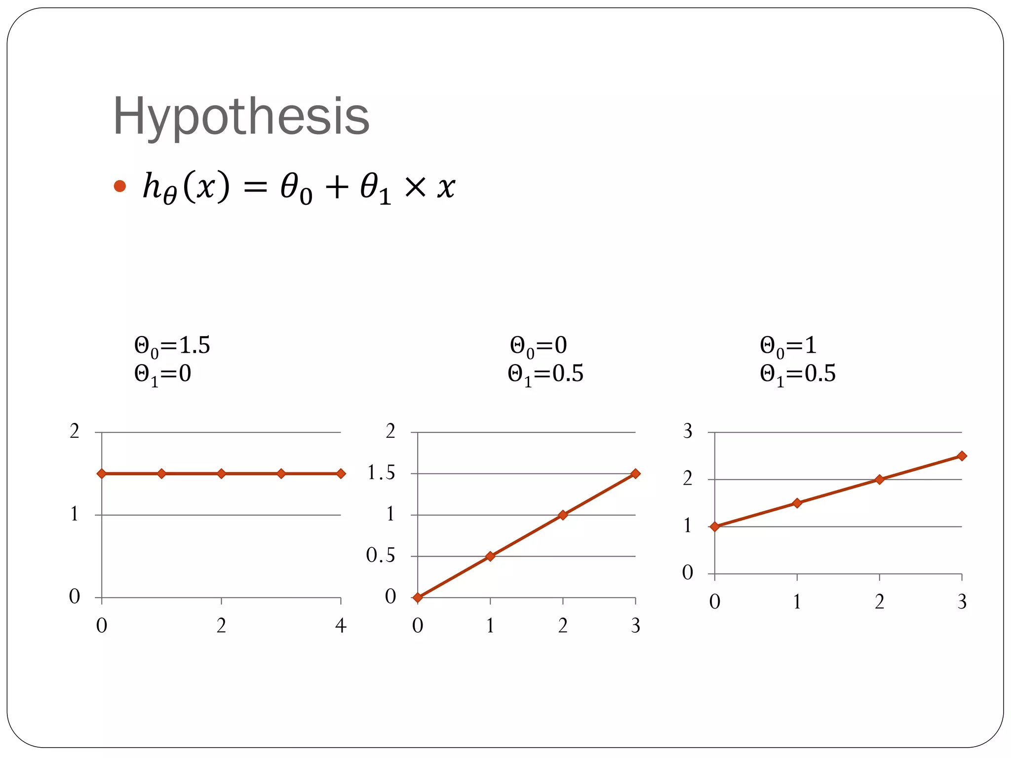
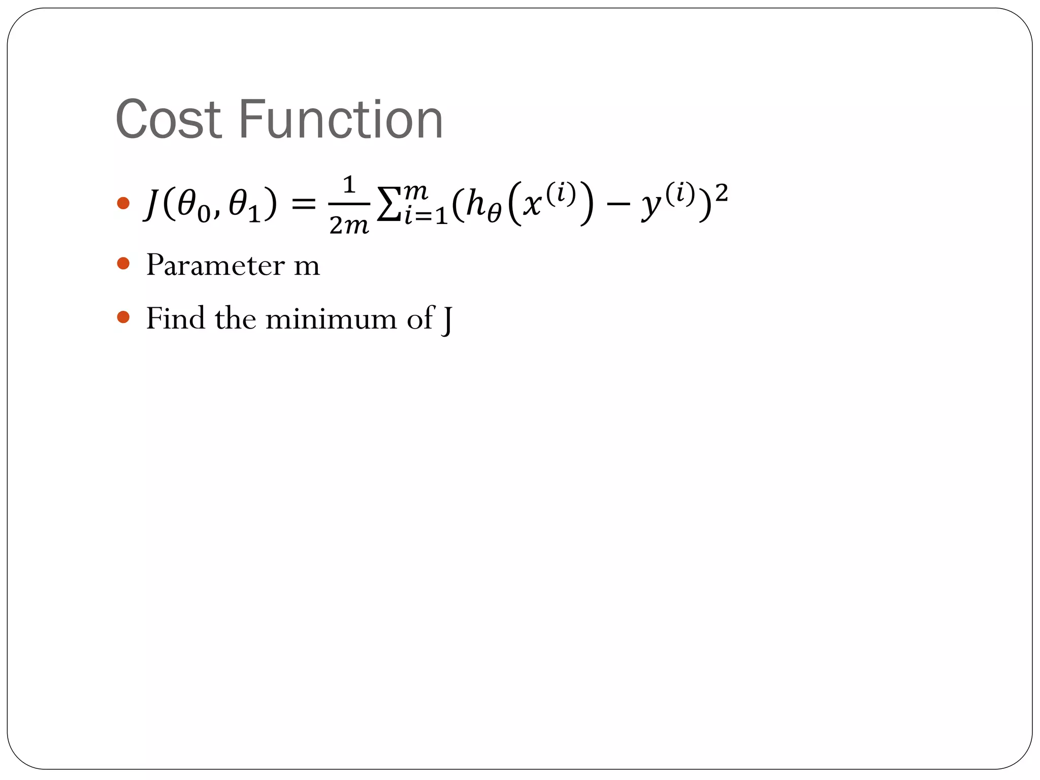
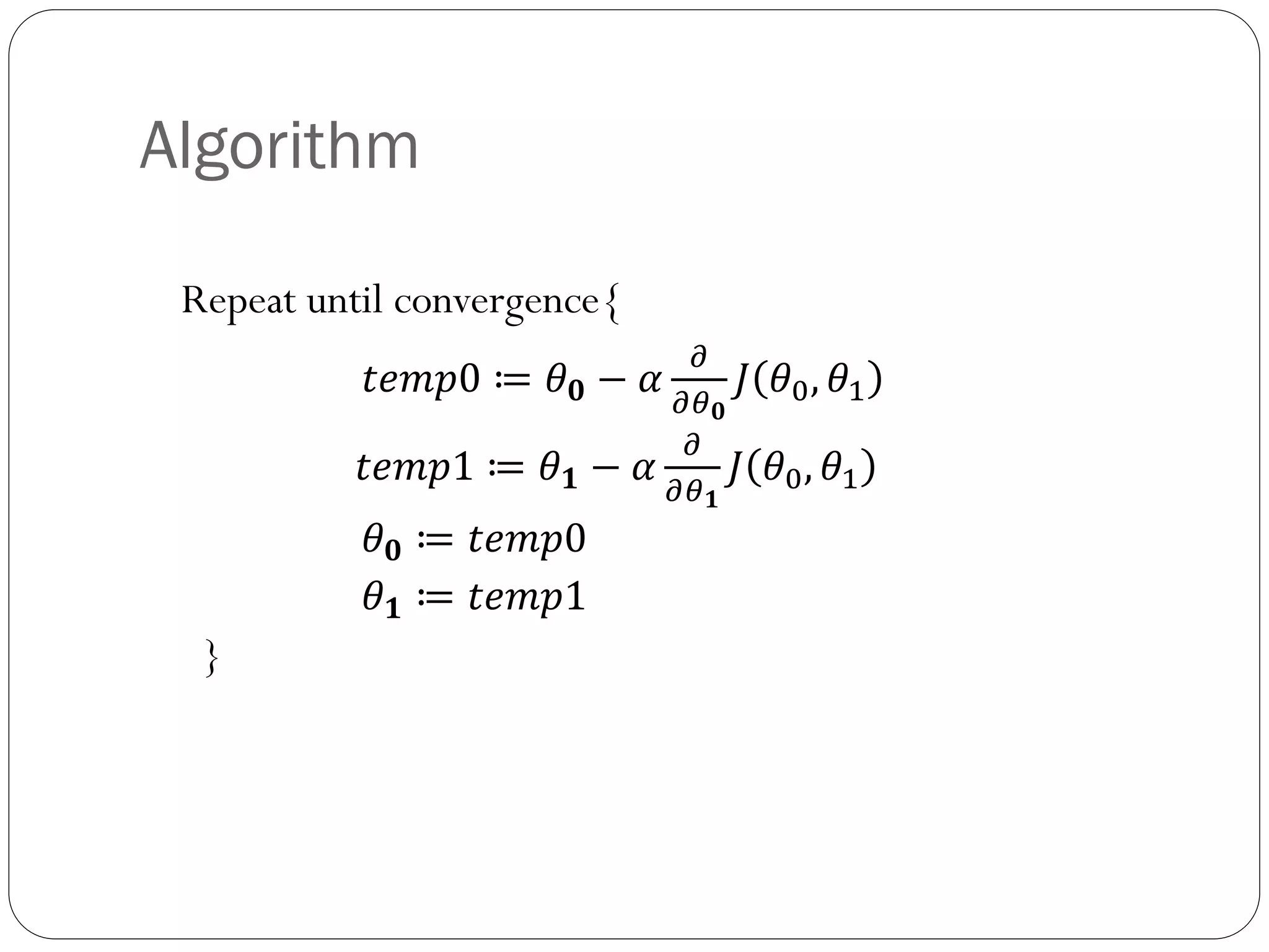
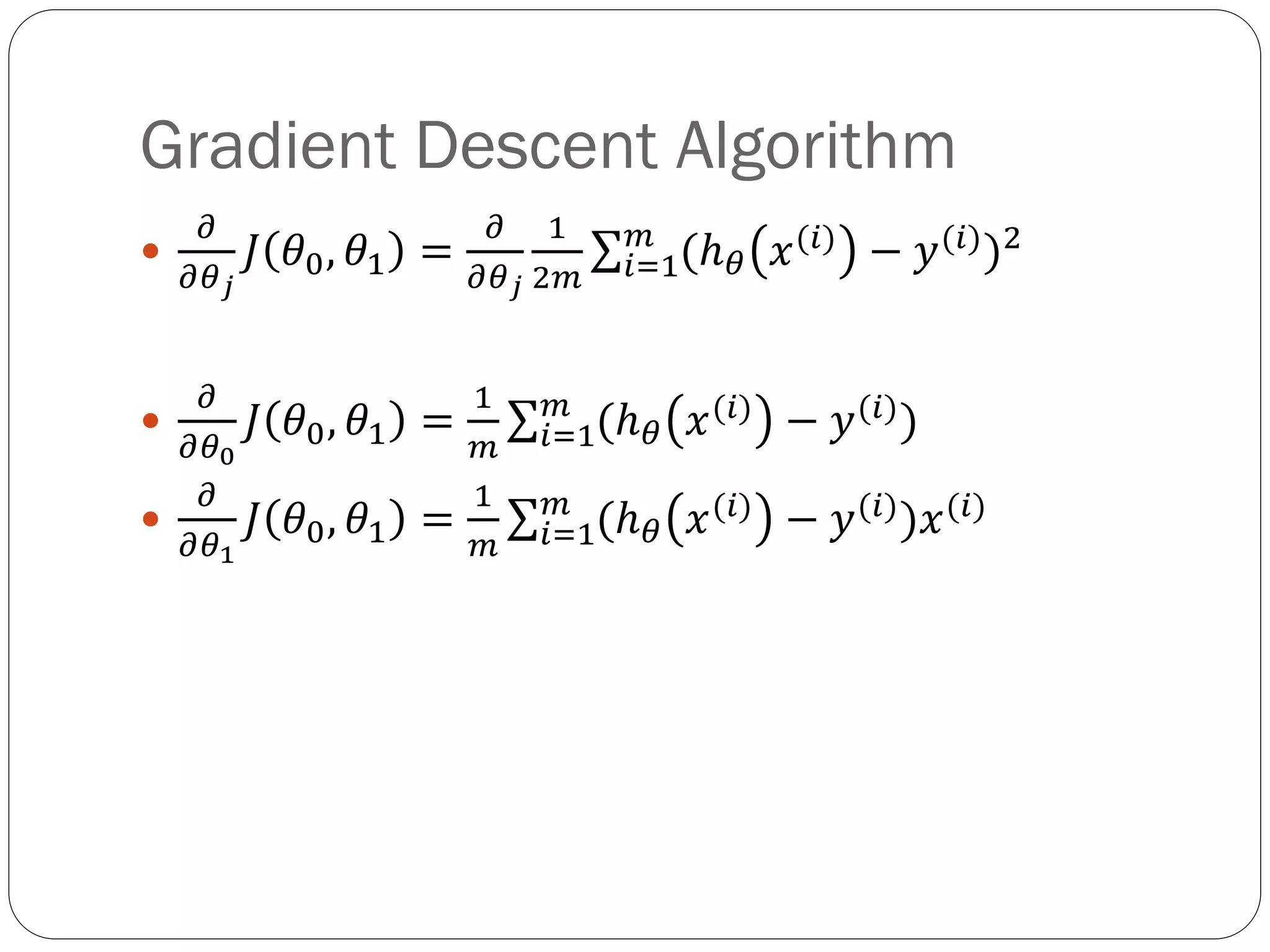
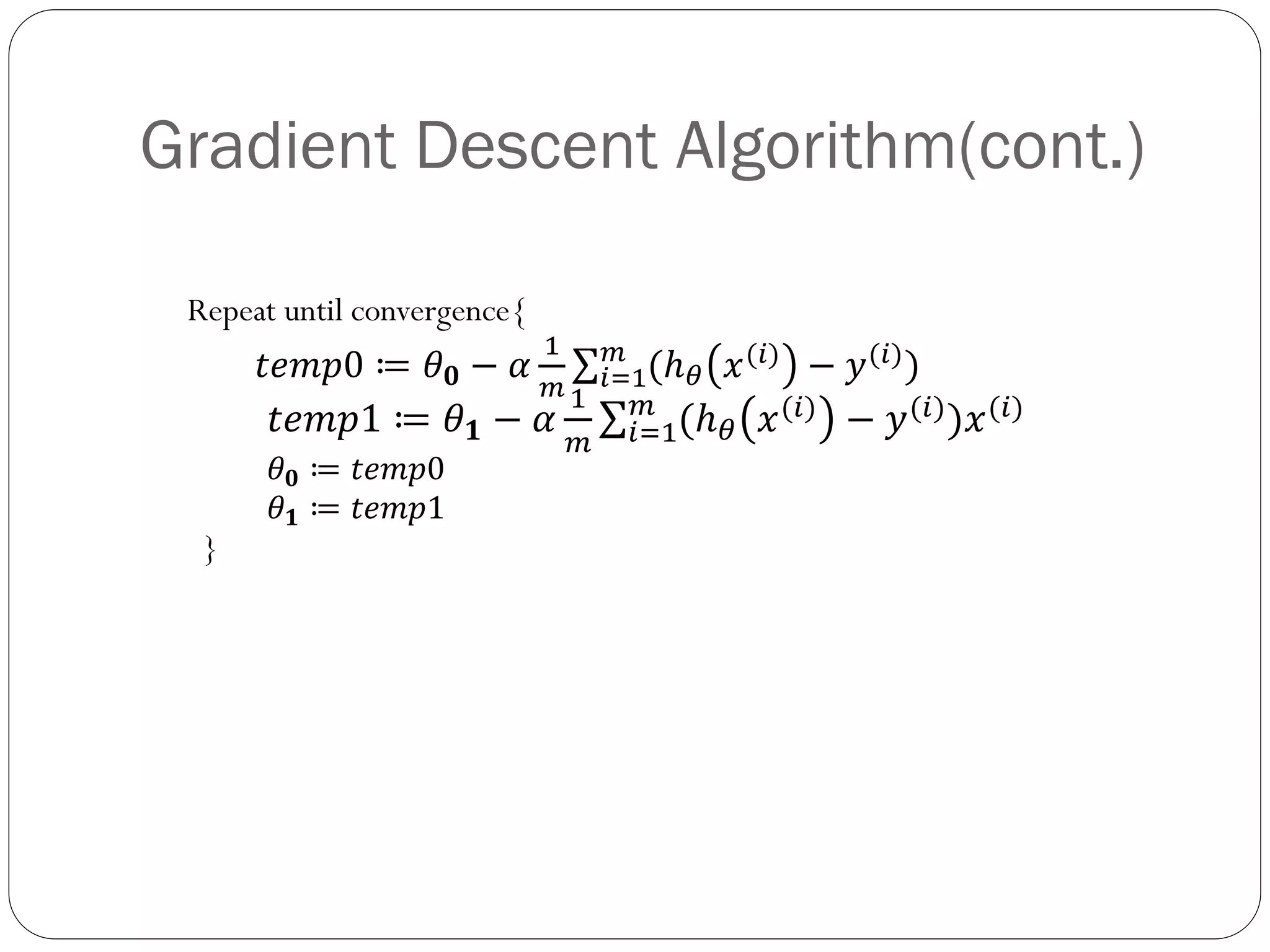
This document introduces linear regression with one variable to predict house prices based on size. It describes using an algorithm called gradient descent to find the parameters theta-0 and theta-1 that minimize the cost function J and best fit the linear hypothesis h to the training data. The algorithm repeats updating the parameter values temp-0 and temp-1 by subtracting a fixed learning rate alpha times the partial derivative of J with respect to each parameter, until convergence is reached.

1. Linear Regression with One Variable

2. Predict the Price of the House
Area x(i) Price y(i)
2104 460
1416 232
1534 315
852 172
Size of House
x
Estimated
Price y
Training Set
Learning
Algorithm
Hypothesis h

3. Hypothesis
 ℎ 𝜃 𝑥 = 𝜃0 + 𝜃1 × 𝑥
0
1
2
0 2 4
0
0.5
1
1.5
2
0 1 2 3
Θ0=1.5 Θ0=0 Θ0=1
Θ1=0 Θ1=0.5 Θ1=0.5
0
1
2
3
0 1 2 3

4. Cost Function
 𝐽 𝜃0, 𝜃1 =
1
2𝑚 𝑖=1
𝑚
(ℎ 𝜃 𝑥(𝑖)
− 𝑦(𝑖)
)2
 Parameter m
 Find the minimum of J

5. Algorithm
Repeat until convergence{
𝑡𝑒𝑚𝑝0 ≔ 𝜃 𝟎 − 𝛼
𝜕
𝜕𝜃 𝟎
𝐽 𝜃0, 𝜃1
𝑡𝑒𝑚𝑝1 ≔ 𝜃 𝟏 − 𝛼
𝜕
𝜕𝜃 𝟏
𝐽 𝜃0, 𝜃1
𝜃 𝟎 ≔ 𝑡𝑒𝑚𝑝0
𝜃 𝟏 ≔ 𝑡𝑒𝑚𝑝1
}

6. α
 Small α
 Too large α
 Fixed

7. Gradient Descent Algorithm

𝜕
𝜕𝜃 𝑗
𝐽 𝜃0, 𝜃1 =
𝜕
𝜕𝜃 𝑗
1
2𝑚 𝑖=1
𝑚
(ℎ 𝜃 𝑥(𝑖) − 𝑦(𝑖))2

𝜕
𝜕𝜃0
𝐽 𝜃0, 𝜃1 =
1
𝑚 𝑖=1
𝑚
(ℎ 𝜃 𝑥(𝑖)
− 𝑦(𝑖)
)

𝜕
𝜕𝜃1
𝐽 𝜃0, 𝜃1 =
1
𝑚 𝑖=1
𝑚
(ℎ 𝜃 𝑥(𝑖)
− 𝑦(𝑖)
)𝑥(𝑖)

8. Gradient Descent Algorithm(cont.)
Repeat until convergence{
𝑡𝑒𝑚𝑝0 ≔ 𝜃 𝟎 − 𝛼
1
𝑚 𝑖=1
𝑚
(ℎ 𝜃 𝑥(𝑖)
− 𝑦(𝑖)
)
𝑡𝑒𝑚𝑝1 ≔ 𝜃 𝟏 − 𝛼
1
𝑚 𝑖=1
𝑚
(ℎ 𝜃 𝑥(𝑖)
− 𝑦(𝑖)
)𝑥(𝑖)
𝜃 𝟎 ≔ 𝑡𝑒𝑚𝑝0
𝜃 𝟏 ≔ 𝑡𝑒𝑚𝑝1
}