1. Chapter 1
Control Problem and Control Actions
1.1 Control problem
In any control system, where the dynamic variable has to be maintained at the desired set point
value, it is the controller which enables the requirement of the control objective to be met.
The control design problem is the problem of determining the characteristics of the controller so
that the controlled output can be:
1. Set to prescribed values called reference
2. Maintained at the reference values despite the unknown disturbances
3. Conditions (1) and (2) are met despite the inherent uncertainties and changes in the plant
dynamic characteristics.
4. Maintained within some constrains.
The first requirement above is called Tracking or stabilization depending on whether the set-
point continuously changes or not, The second condition is called disturbance rejection. The third
condition is called Robust tracking/stabilization and disturbance rejection. The fourth condition is
called optimal tracking/stabilization and disturbance rejection.
1
1
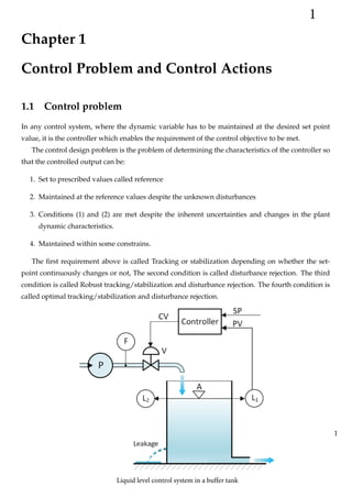
Liquid level control system in a buffer tank
2. 1.1.1 Control assessment framework
Control systems may be assessed in terms of 1. Stability, 2. Reference tracking and 3.
Disturbance rejection.
Consider the system in the figure below;
We want to discuss and assess control system performance in terms of stability, reference
tracking and disturbance rejection
System response as a function of inputs:
θo = θd + G1U but U = KE and E = θi − θo
Therefore θo = θd + G1K(θi − θo)
So θo(s) =
G1(s)K(s)
1 + G1(s)K(s)
θi(s) +
1
1 + G1(s)K(s)
θd(s)
Three properties of interest are:
• Closed-loop system stability:- Depends upon making sure that the poles of 1 +
G1(s)K(s) are in LHP of s-plane
• Reference tracking performance:- Looks at the shape of time response (Speed,
overshoot and steady state errors)
• Disturbance rejection performance:- Looks at speed of response , size of peak
disturbance and make sure that no steady state error due to disturbance.
Consider the following transfer function which represents a heating system
θo(s) = G1(s)U(s) Where G1(s) =
0.3
2s + 1
2
3. The input signal U(s) is the power in KW from the heater and the output signal θo(s) is
the resulting temperature. The time constant of the system is 2 hours
We wish to control the system behaviour. So we use proportional controller and unity
feedback. Assume that the reference signal is a unit step input and the disturbance is given
by θd(t) = 0.5
Control assessment of the system
• Closed-loop system stability and response:-
Open-loop transfer function
Go(s) = G1(s)Kp =
0.3Kp
2s + 1
There is single open-loop pole at s = −0.5
Closed-loop transfer function
GCL(s) =
G1(s)K(s)
1 + G1(s)K(s)
=
0.3Kp
2s + 1 + 0.3Kp
So there is single closed-loop pole at s = −0.5 − 0.15Kp
The System is stable for positive values of Kp
• Reference tracking performance:- Output response to reference input
G1(s)K(s)
1 + G1(s)K(s)
θi(s)
θo(s) = GCL(s)θi(s) =
Final value theorem gives
θo ss = lim
s→0
sθo(s) = lim
s→0
s
G1(s)K(s)
1 + G1(s)K(s)
θi(s)
For this system , the steady state response
θo ss = lim
s→0
s
0.3Kp
1
2s + 1 + 0.3Kp s
=
0.3Kp
1 + 0.3Kp
3
4. This implies that the steady state error reduces as Kp increases.
In reality , there will be physical limitations on gain. ie actuator may not deliver
(Actuator saturation.)
Pole plot and response is as below
The response speeds up with increasing Kp
• Disturbance rejection performance:-
Output response to disturbance input
θo(s) =
1
1 + G1(s)K(s)
θd(s)
For this system:
θo(s) =
2s + 1
2s + 1 + Kp
0.5
s
Taking inverse transforms gives the disturbance time response
θo(s) =
0.25Kp
0.5 + 0.15Kp
1 + 0.3Kpe−(0.5+0.15Kp)t
As K becomes larger, the steady state value of the disturbance response gets smaller
and the speed of response increases
4
5. 1.2 Control actions
Given a general plant as shown Fig. 1.1 The manner in which the automatic controller produces the
Figure 1.1: A general plant.
control signal is called the control action.
The control signal is produced by the controller, thus a controller has to be connected to the
plant. The configuration may take either Close loop or Open loop as shown in Fig.1.2 and 1.3.
Figure 1.2: Close loop Controlled system.
Figure 1.3: Open loop Controlled system.
5
6. 1.2.1 Basic control actions
Control actions may be further classified into control modes namely:
• Discontinuous control mode: In discontinuous controllers, the manipulated variable y (Con-
trol signal) changes between discrete values. Depending on how many different states the
manipulated variable can assume, a distinction is made between two-position, three-position ,
multi-position controllers and floating controller. Compared to continuous controllers,discontinuous
controllers operate on very simple switching of final controlling elements. If the system contains
energy storing components, the controlled variable responds continuously, despite the step
changes in the manipulated variable. If the corresponding time constants are large enough, good
control results at small errors can even be reached with discontinuous controllers and simple
control elements.
• Continuous control mode:In continuous controllers, the manipulated variable can assume
any value within the controller output range. The characteristic of continuous controllers
usually exhibits proportional (P), integral (I) or differential (D) action
• Composite mode: The characteristic of Composite controllers usually exhibits combinations
of proportional (P), integral (I) or differential (D) action.
Figure 1.4: Control actions.
6
7.
€ ‚
ƒ
ƒ
„
† ‡€
ˆ ‡
‚‰
Š
‹
†
†
Controller
O/P
P
( )
ON
100%
OFF
0%
Neutral Zone
error
e
( )
1 Two point control mode (Bang-Bang controller)
1.3 DISCONTINUOUS CONTROLLER MODES
7
1
100%
50%
0
– e1 + e1
0
error
(e)
Controller
0/P
P
e2
10.
Controller
o/p
P 100%
0%
100 % Saturation
0% Saturation
error
(e)
P.B
7
t
t
t = t1
error
(e)
Controller
o/p
P
=
t t1
€‚
ƒ
10
Controller Process
R s
( ) E s
( ) P s
( )
kp C s
( )
1
1 + TS
Fig. 2.3
11. m dd p dd
pp l ll d€ l l lm pp l
e d pb bpp
lpble d ld
‚
ƒ
ƒ
„
ƒ
†
€ ‚
1
ƒ „
Controller
o/p
kF
– kF
0
o
error
e
( )
dp
dt
e
P
ƒ
† ‡
†ˆ
‡
11
12.
€ ‚ ‚ƒ„
‚
†
‚ ‚
‚
†
1
T s
i
E s
( ) P s
( )
‡
ˆ ‰
‚Š‚
‹
‚ Œ
12
A
Ti
t
error
e
A
Controller
o/p P
=
t t1
t
13.
R s
( )
P s
( ) 1
1 + Ts
C s
( )
1
Tis
(Integral Mode) (Process)
1
Tis
Kp 1 +
P S
( )
E S
( )
error
(e)
P-only
I-only
+
P I
only
P + I Action
{
t = t1
t
t
t
t
t = t1
t = t1
t = t1
A
t
P K A
= +
p
AKp
Ti
€ ‚
13
14. R( )
1
1 + T
C( )
+
P I controller (Process)
{
{
1
T
Kp 1 +
€
14
13 Derivative
Unlike P-only and I-only controls, D-control is a form of feed forward control.
D-control anticipates the process conditions by analyzing the change in error.
It functions to minimize the change of error. The primary benefit of D
controllers is to resist change in the system, the most important of these being
oscillations. The control output is calculated based on the rate of change of the
error with time. The larger the rate of the change in error, the more pronounced
the controller response will be.
D-control correlates the controller output to the derivative of the error. This
D-control behavior is mathematically illustrated in Equation
p(t) = Td
de
dt Where • p(t) = controller output
• Td = derivative time constant
• de = change in error
• dt = change in time
15. Mathematically, derivative control is the opposite of integral control.
Although I-only controls exist, D-only controls do not exist. D-
controls measure only the rate of change in error. D-controls do not
know where the setpoint is, so it is usually used in conjunction with
another method of control, such as P-only or a PI combination
control. D-control is usually used for processes with rapidly changing
process outputs. However, like the I-control, the D control is
mathematically more complex than the P-control. Since it will take a
computer algorithm longer to calculate a derivative or an integral than
to simply linearly relate the input and output variables, adding a D-
control slows down the controller’s response time.
Unlike proportional and integral controllers, derivative controllers do
not guide the system to a steady state because they do not act when
error does not change even in presence of the error. Because of this
property, D controllers must be coupled with P, I or PI controllers to
properly control the system.
€ ‚ƒ
„
„
†
Kp (1 + d
T S)
P S
( )
E S
( )
16. R( ) (1 +
K T
p ) 1
1 + T
Controller Process
€
‚
ƒ„
€
†
‡ ƒ
ˆ
error
(e)
P-only
D-only
+
P D
Action
P + D Action
{
t
t
t
t
At
t = t1
t = t1
t = t1
t = t1
15
17. Characteristics of + + controller
€
€
‚ƒ ‚
„ †‡
ˆ
‰
†
†
Š‹ Œ
1.5.3 Proportional + Integral + Derivative Controller
Mode
[+ + Mode]
1
T S
i
Kp 1 +
P S
( )
E S
( )
+ d
T S
16