SlideShare a Scribd company logo
1 of 25
Experiments, Results and Analyses 2:
     Understanding Self and Cooperative Learning in a Multiagent System

                                   Leen-Kiat Soh and Juan Luo

                         Computer Science and Engineering Department
                                     University of Nebraska
                          115 Ferguson Hall, Lincoln, NE 68588-0115
                           tel: (402) 472-6738 fax: (402) 472-7767
                                e-mail: { lksoh, luo}@cse.unl.edu

                                         August 12, 2002

1.     INTRODUCTION

This document extends our previous report “Experiments, Results and Analyses: Understanding
Self and Cooperative Learning in a Multiagent System”. We report on our experiments with a
multiagent system with initial case bases of different sizes. Specifically, agent A1 is given an
initial case base of only two cases, while other agents (A2, A3, and A4) are given 16 cases each.
The objective is to see how agent A1 learns new cases in the face of such “knowledge
starvation.”

In our previous report, we drew the following conclusions. In this report, we have conducted
experiments to understand the role of self and cooperative learning in a multiagent system. We
have shown that the combine learning (cooperative + self) in general results in a wider coverage
than does the self-only learning for most problem descriptors of the cases. We have also
observed problem space shifting, focusing, and expanding in our learning behavior, and that
cooperative learning’s ability to introduce more diversity into the casebase than just self learning
alone. We have also concluded that each cooperatively learned new case brings about a higher
utility gain and difference gain to the casebase, implying that the impact of these external or
foreign cases is very significant when an agent learns. In addition, combine learning brings
about a higher utility gain, difference gain, and utility slope than self learning only.
Furthermore, drawing from the results of the second stage of our experiments, we have realized
that the combine learning at the second stage is able to bring in more diversity to the casebase
when the initial casebase has been grown using both self and cooperative learning. However, the
utility gain and slope seem to be unaffected at the second stage regardless of the initial
casebases. This indicates that the combine learning is consistent in bring in useful cases
regardless of the initial casebases yet is able to increase the diversity of the casebase at the same
time.

In this report, we study agent A1’s learning behavior as compared to other agents, and also
investigate whether there are observable patterns or differences between this multiagent system
and the one we used in our previous report.

2.     SOME DETAILS


                                                 1
In this current design, we add a new idea for the chronologically-ordered casebase. Specifically,
we make the resolution of case forgetting more precise by introducing the idea of a birthdate.

In our previous design, when the size of a casebase reaches a certain value
(=MAX_CASE_BASE_SIZE), every new case added may result in the deletion of an unused,
old case. Thus, when the size of the initial casebase for an agent is close to or the same as
MAX_CASE_BASE_SIZE, the agent will start the deletion immediately, without giving those
cases an opportunity to become useful or to be used. That is, as soon as the system starts
encountering a new case, one of the unused, old case will be deleted. In addition, suppose the
size of the casebase reaches MAX_CASE_BASE_SIZE, while all old cases have been used.
Now, when a new case is added, since there is not any unused, old case, no deletion is carried
out. But, when the next new case is added, the new case that is previously added may not have a
chance to be used yet, and thus, it is now an unused, old case that may be deleted! So, once
again, we do not give the newly added cases an opportunity to become useful or to be used.

Our approach to solve the problem is two-layered. First, we add a new attribute to each case: a
“timestamp” to represent the “birth date” of a case. So, initially, when the system reads in the
casebases, each case is assigned the same birth date. We provide the operating-system-based
timestamp through our UtilNTP::getCurrentTime() method. Second, we use the following
decision making process for case deletion and replacement:

1.     If the size of the casebase reaches MAX_CASE_BASE_SIZE, then consider case
       deletion.
(a)    Find the oldest, unused case in the casebase.
(b)    currentTimeStamp = UtilNTP::getCurrentTime()
(c)    If the difference between the currentTimeStamp and the timestamp of the oldest, unused
       case is at least N seconds, then delete the case.
(d)    Otherwise, go to step (2).

2.     If case replacement cannot be carried out, then simply add the new case if it is important,
       useful, or different enough.

At first glance, the search for the oldest, unused case in the casebase may seem to be a time
consuming task. However, note that our casebase is a vector. A new case is always added to the
end of the vector. Thus, we only have to scan the vector from the front until we hit the first
unused case. That will be the oldest, unused case.

There is also another problem associated with the implementation. When an existing case is
replaced by a new case, the previous design simply put the new case at the place of the existing
case in the vector. Since this messed up the chronological order of the cases, our replacement is
implemented in two steps: (1) delete the existing case, (2) add the new case to the end of the
vector. In this manner, the vector of cases is always ordered chronologically.

Finally, with this new implementation, we can now look at the age of a case. If it is too young,
then we give it a chance to be used. If it is too old and still not useful, then we can delete it.


                                                2
3.          EXPERIMENT SETUP

3.1.        Randomizations

See the previous report.

3.2.CaseBase

Agents have different casebases. Agent A1 has an initial casebase of two cases. Agents A2, A3,
and A4 each has the same initial casebase of 16 cases.

3.3.        Design

See the previous report. . In the following, we refer to C i as the initial casebase, C f as the final
casebase after the first stage, and C ′f as the final casebase after the second stage. Experiment 1
uses both self and cooperative learning (combine learning) for both stages. Experiment 2 uses
only self-learning for the first stage and combine (self + cooperative) learning for the second
stage.

4.          RESULTS AND ANALYSES

4.1.   Experiment 1 vs. Experiment 2: C i and C f
Table 1 shows the results of C i and C f of the two sets of experiments for the initiating
casebases, looking only at the problem descriptors.

                A1     Exp1   Exp2   A2      Exp1       Exp2   A3     Exp1     Exp2    A4      Exp1    Exp2
                Ci     Cf     Cf     Ci      Cf         Cf     Ci     Cf       Cf      Ci      Cf      Cf
#task (ave)     6.5    2.5    1.64   4.38    3.12       2.3    6      3.86     3.9     5.38    3.1     3.27
#task           4.95   2.33   2.56   2.68    2.57       2.61   3.1    3.46     3.51    2.8     3.03    3.1
(std.dev)
#partner        1      2.72   2.64   2.25    2.5        2.47   2.25   2.57     2.5     2.25    2.43    2.6
(ave)
#partner        0      0.67   0.74   1.77    1.37       1.17   1.77   1.37     1.4     1.77    1.14    1.33
(std.dev)
speed (ave)     1.75   1.06   1.16   2.33    1.73       1.49   2.36   1.81     1.72    3.19    1.94    2.1
speed           1.77   0.81   0.76   1.22    1.22       1.26   1.16   1.14     1.25    1.54    1.60    1.68
(std.dev)
timeAllowe      5000   7302   7781   5125    6368       4940   5125   6284     5352    5125    6395    5778
d (ave)
timeAllowe      1414   3754   4104   2277    3755       3065   2277   3586     3335    2277    2902    3733
d (std.dev)

 Table 1 The results of the initial and final casebases after going through non-selective learning for two
sets of experiments, initiating casebases. Exp1 uses both the cooperative and self- learning mechanisms.
                                Exp2 uses only the self-learning mechanism.


                                                    3
Based on Table 1, we observe the same patterns or trends as reported in Section 4.1 of our
previous report. Briefly, we see problem space shifting, focusing, and expanding. We also see
that the combine learning tends to result in a higher coverage than self-only learning, implying
that the cooperative learning is able to introduce more diversity to the casebase, as expected.

Table 2 shows the results of C i and C f of the two sets of experiments for the responding
casebases, looking only at the problem descriptors.

              A1     Exp1    Exp2     A2      Exp1        Exp2    A3     Exp1    Exp2   A4     Exp1     Exp2
              Ci     Cf      Cf       Ci      Cf          Cf      Ci     Cf      Cf     Ci     Cf       Cf
#task (ave)   4      1.75    1.33     4.56    2.9         3.27    4.75   2.83    2.57   6.13   2.63     3.2
#task         4.24   1.73    1.87     2.19    2.48        2.44    2.93   2.83    2.8    2.94   2.47     3.2
(std.dev)
CpuUsage      0.63   0.35    0.31     0.6     0.42        0.5     0.6    0.41    0.42   0.6    0.43     0.5
(ave)
cpuUsage      0.35   0.25    0.22     0.26    0.31        0.3     0.26   0.3     0.28   0.26   0.31     0.3
(std.dev)
power (ave)   0.35   0.86    0.89     0.36    0.7         0.61    0.36   0.67    0.68   0.36   0.74     0.67
power         0.5    0.34    0.29     0.41    0.44        0.45    0.41   0.44    0.45   0.41   0.44     0.45
(std.dev)
maxCPUGi      2.5    10.2    10.2     2.75    9.1         5.44    2.75   8.4     7.77   2.75   9.62     8.0
veUp (ave)
maxCPUGi      3.54   8.1     6.46     3.44    7.6         6.45    3.44   8.1     6.48   3.44   7.96     8.67
veUp
(std.dev)
timeAllowe    7000   14935   9021     6625    10866       9554    6625   11488   6371   6625   14271    7158
d (ave)
timeAllowe    1414   21318   7233     2277    19532       14421   2277   19101   4384   2277   23607    4676
d (std.dev)

  Table 2 The results of the initial and final casebases after going through non-selective learning for two
sets of experiments, responding casebases. Exp1 uses both the cooperative and self learning mechanisms.
                                Exp2 uses only the self learning mechanism.

Based on Table 2, we observe the same patterns or trends as reported in Section 4.1 of our
previous report. Briefly, we see problem space shifting, focusing, and expanding. We also see
that the combine learning tends to result in a higher coverage than self-only learning, implying
that the cooperative learning is able to introduce more diversity to the casebase, as expected.

Comparing the two casebases, we see that the combine learning (cooperative + self) in general
results in a wider coverage than does the self-only learning.

Overall, we also have the same conclusions as those in Section 4.1 of our previous report.

4.2.     Experiment 1 vs. Experiment 2: Gains


                                                      4
Table 3 shows the utility and diversity gains of the agents’ learning steps for Experiment 1, in
which both the self and cooperative learning mechanisms are active. Appendix A’s Tables 1-4
are the raw data that we use to compute for Table 3.

Initiating CaseBase Self           Coop        Ave               RespondingCaseBase Self           Coop        Ave
#learnings                  164           15          179        #learnings                 126           42         168
#new cases                   44            9           53        #new cases                  47            9          56
avg util gain          0.099329 0.042267 0.094547                avg util gain          0.177671    0.08166 0.153668
max util gain                2.5     0.3518            2.5       max util gain            2.2222     0.7143      2.2222
min util gain              -0.85    -0.4167          -0.85       min util gain                -1    -0.7958           -1
#util gain>0.400000          19            0           19        #util gain>0.400000         24            5          29
#util gain<-0.200000          6            2            8        #util gain<-0.200000        15            4          19
avg diff gain           0.13794 0.083967 0.133417                avg diff gain          0.053305 0.020805       0.04518
max diff gain            4.6464      0.2309      4.6464          max diff gain            0.4254      0.228      0.4254
min diff gain           -0.3766     -0.2747     -0.3766          min diff gain           -0.4266    -0.3445      -0.4266
#diff gain>0.400000           5            0            5        #diff gain>0.400000          2            0           2
#diff gain<-0.200000          2            1            3        #diff gain<-0.200000         9            3          12
sizeslope              0.285498 0.294587        0.28626          sizeslope              0.323335    0.30215 0.318039
difslope               0.053601     0.05764     0.05394          difslope               0.044596 0.037471 0.042815
utislope               0.089857 0.073333 0.088472                utislope               0.159825 0.160157 0.159908

Table 3 The utility and difference gains of the agents’ learning steps for Experiment 1, in which both self
                            and cooperative learning mechanisms are active.

The utility of a casebase is compiled from the usage history of the cases of the casebase: the
number of times a case is used and the degree of success of each case. Please refer to our
previous report for the detailed description of our utility computation.

Note that for the computation of difference values, we attempted with ( n 2 − n ) 2 as sizeofcasebase.
However, as n increases, sizeofcasebase grows polynomially, and reduces the difference values
significantly. Thus, we decide to revert back to the original design: sizeofcasebase is the
number of cases in the casebase.

From Table 3, we observe the same patterns or trends as those reported in Section 4.2 of our
previous report: (1) self learning occurs more often than cooperative learning, (2) in general, a
responding casebase “grows” better than an initiating casebase, and (3) in both casebases, the
number of new cases learned via cooperative learning is much smaller than that learned via self-
learning.

In our previous report, we observed that the cooperative learning had a higher average utility
gain for the initiating casebase. But here we see that the cooperative learning had a lower
average utility gain. As we shall learn later, this is due to the fact that agent A1 has a negative
value for its average utility gain for both the initiating casebase and the responding casebase. So,
in this we see the first impact of A1’s unique property (with a very small initial casebase) on the


                                                             5
overall system. The possible reason for the negative utility gain is that due to the extremely
small initial casebase, the agent is unable to recruit good, foreign cases in such a short time. This
is because the recruit is based on the existing cases in the casebase. So, if the existing cases are
very limited in their coverage, it is not easy to recruit foreign cases that can expand the coverage
of the casebase. Thus, in the short run, the cooperative learning’s utility gain is negative. On the
other hand, the agent is more capable in self-learning. Self-learning is motivated by the events
the agent encounters. And thus, it is problem-driven and dynamic and allows the agent to cover
more grounds given such a small casebase. Thus, we see that the agent has a much higher utility
for its self-learning than its cooperative learning (Table 5).

Table 4 shows the utility and diversity gains of the agents’ learning steps for Experiment 2, in
which only the self-learning mechanism is active. Appendix B’s Tables 1-4 are the raw data that
we use to compute for Table 4.

                                      Initiating             Responding
          #learnings                  266                                       208
          #new cases                  50                                         47
          avg util gain               0.072247                            0.138455
          max util gain               2.3333                                      5
          min util gain               -1.3333                                    -4
          #util gain>0.400000         23                                         75
          #util gain<-0.200000        11                                         17
          avg diff gain               0.083246                            0.034295
          max diff gain               4.6372                                 0.3338
          min diff gain               -0.3418                               -0.3704
          #diff gain>0.400000         4                                           0
          #diff gain <-0.2000         2                                           7
          Sizeslope                   0.179503                            0.215719
          Difslope                    0.030031                            0.034295
          Utislope                    0.068218                            0.138455

Table 4 The utility and difference gains of the agents’ learning steps for Experiment 2, in which only self
                                            learning is active.

Table 4 shows the utility and difference gains for the agents when only self learning is used.
Comparing Tables 3 and 4, we observe the same patterns and trends as reported in Section 4.2 in
our previous report:

1. The average utility gain for combine learning (Experiment 1) is higher than self-only
   learning (Experiment 2): 0.094547 to 0.072247 in the initiating casebase, and 0.153668 to
   0.138455 in the responding casebase.
2. The average difference gain for combine learning (Experiment 1) is higher than self-only
   learning (Experiment 2): 0.133417 to 0.083246 in the initiating casebase, and 0.04518 to


                                                    6
0.034295 in the responding casebase. So, once again, the combine learning is able to learn
   more diverse cases.
3. Looking at the slopes, we also see that the combine learning has a higher slope in the number
   of cases in the casebase (adds new cases more effectively) and in the utility (uses cases more
   effectively). In initiating casebases, the numbers are 0.28626 to 0.179503 and 0.088472 to
   0.068218, respectively. In responding casebases, the numbers are 0.318039 to 0.215719 and
   0.159908 to 0.138455, respectively. This shows that the agents with combine learning are
   able to learn new cases more effectively and uses cases in their casebases more effectively as
   well.
4. Looking at the difference slopes, we see that the combine learning has a significantly higher
   slope than self-only learning: 0.05394 vs. 0.030031 for initiating casebases, 0.042815 vs.
   0.034295 for responding casebases, respectively. This is due to the fact that by importing
   cases from other agents, an agent is able to introduce more diversity into its own casebase.
   Thus, we have observed results that are expected of combine learning in this measurement.

Now, we look at agent A1 specifically, referring to Table 5 and Table 3. .

Initiating Case                                    Responding Case
Base                                               Base
                  Self       Cooperative                             Self        Cooperative
#learnings              42           5        47   #learnings             30              10        40
#new cases              11           4        15   #new cases             11               3        14
avg util gain      0.1641      -0.0898 0.137089    avg util gain      0.3469         -0.1078 0.233225
Max util gain          2.5      0.2721       2.5   max util gain      2.2222          0.7143    2.2222
min util gain        -0.85     -0.4167     -0.85   min util gain          -1         -0.7958        -1
#util                                              #util
gain>0.400000            9          0         9    gain>0.400000            13            2        15
#util                                              #util
gain<-0.200000          6            2         8   gain<-0.200000          8              3        11
avg diff gain      0.0686       0.1428 0.076494    avg diff gain      0.0683         0.0593   0.06605
Max diff gain      0.5891       0.2309    0.5891   max diff gain      0.3543         0.1993    0.3543
min diff gain           0      -0.0021         0   min diff gain           0              0         0
#diff                                              #diff
gain>0.400000            1          0         1    gain>0.400000             0            0         0
#diff                                              #diff
gain<-0.200000          0           0        0     gain<-0.200000          0              0         0
sizeslope          0.3261      0.3333 0.326866     sizeslope          0.3514          0.359    0.3533
difslope           0.0653      0.0651 0.065279     difslope           0.0639         0.0662 0.064475
utislope           0.1256      0.0882 0.121621     utislope           0.2551          0.242 0.251825

Comparing the following Table 3 and Table 5, we observe the following:
1. Agent A1 does not learn faster than the other three agents. In terms of learning experiences
   (#learnings), the numbers are about the same. This is expected since the agents encounter
   similarly dynamic events in the same environment. In terms of the number of new cases
   added, the numbers are also about the same. That means even with a much smaller casebase,
   agent A1 does not add more cases into its casebase. In one way, this is expected: all agents
   are picky in what they learn. That given a very small casebase does not necessarily give an
   agent to add whatever cases it encounters. On the other hand, this is not expected. An agent


                                                    7
with a very small casebase should be more willing to learn more cases. This is actually true
     as we do have the MAX_CASE_BASE_SIZE mechanism that prevents a casebase to grow
     out of control. So, yes, if we let the system run long enough, we would see that agent A1
     will learn more cases and slow down after reaching the threshold, while all the other agents
     will start slowing down much earlier as they already have more cases to begin with. We do
     see that agent A1 has a slightly higher sizeslope value than all the other agents, in general.
2.   Overall, agent A1 learns better than the other three agents. The average utility gain
     (initiatingCaseBase) for Agent 1 is 0.137089, however, the average utility gain for the 4
     agents is 0.094547. The average utility gain (RespondingCaseBase) for Agent 1 is 0.233,
     however, the average utility gain for the 4 agents is 0.15. Looking at self learning alone, A1
     is much better than the others. This is because A1 starts with such a small casebase, it is
     more likely that (1) most of the cases have been used at least once, and (2) most new cases
     are diverse and useful enough to be added. Looking at cooperative learning alone, A1
     performs much worse than the others. The reason for this has been previously suggested in
     this document.
3.   The number of cooperative learning opportunities is about the same for all agents. Agent A1
     does not attempt to learn more cooperatively. Remember that the trigger for cooperative
     learning is the existence of poor cases in the casebase. With a much smaller casebase, A1
     also has a much smaller number of poor cases. And thus, the logistics of the design
     determines the learning behavior of the agent, a behavior that is not totally expected from the
     viewpoint of machine learning.
4.   For the average diversity gain of the initiating casebase, the self learning of A1 has a much
     smaller gain than all the other agent while the cooperative learning of A1 has a much higher
     gain than all the other agents. This is to be expected. In self learning, the new cases learned
     are the results of a combination of the best case retrieved and the problem at hand. In
     cooperative learning, the new cases learned are foreign cases (triggered by bad cases in the
     casebases but untouched or unaltered when learned). Thus, it is more likely to learn more
     diverse, foreign cases when the agent has very a small casebase, such as A1. By the same
     token, it is less likely to learn more diverse, adapted cases when the agent has a very small
     casebase since its coverage is limited to begin with. Overall, however, there are no
     observable trends for the difslope values for the four agents.
5.   Coupling the observations of (2) and (4), we see that A1’s cooperative learning is able to
     bring more diversity and less utility to its casebase, while its self learning is able to bring
     more utility and less diversity. This is a very interesting and not completely expected
     learning behavior.
6.   Looking only at the slopes of the agents, we see that A1’s self learning, from a global view,
     does have a higher impact than other agents’.
     (a) For the initiating casebase, A1’s utility slope for self learning is 0.1256, as compared to
         0.0670, 0.0869, and 0.0758 of the other three agents. A1’s utility slope for cooperative
         learning is 0.0882, as compared to 0.0651, 0.0893, and 0.0355 of the other three agents.
         So, the cooperative learning is marginally comparable between A1 and the other agents.
     (b) For the responding casebase, A1’s utility slope for self learning is 0.2551, as compared to
         0.1114, 0.1346, and 0.1440 of the other three agents. A1’s utility slope for cooperative
         learning is 0.242, as compared to 0.0974, 0.178, and 0.1361 of the other three agents. So
         we see that the cooperatively learned cases in the responding casebase are more likely to
         be useful than those in the initiating casebase. This is expected since a responding case


                                                 8
has elements of both an initiating agent and a responding agent, and is thus subject to
       more diversity and utility.

4.3.Experiment 1 vs. Experiment 2: Graphs

Appendix C documents the graphs of the agents’ learning record, before the second stage of
agents’ life cycle. In general, the graphs reflect what we have discussed in Section 4.2.
However, Figure 1 provides additional insights. From Figure 1, we see that utility of the
casebase drops after reaching a high value. This is probably due to the convergence. After
learning steadily, an agent hits Phase 3, the precision learning or the refinement learning phase,
as shown in Figure 1. At this phase, the agent learns additional new cases to replace similar,
used cases. Each replacement means removing a case with a nonzero value in #timesOfUsed,
and adding a case with a zero value in #timesOfUsed. Since the utility of the casebase relies on
the values of #timesOfUsed, the utility thus drops. However, it is assuring to see that the utility
of the casebase goes up after each drop, meaning that the agent does learn useful cases.

4.4.Experiment 1 vs. Experiment 2: Impact of Different Initial Casebases, Second Stage

This is the same as the experiments conducted in Section 4.4 of our previous report. Briefly, the
goal of this second stage is to study the impact of different initial casebases. For the first stage,
all agents start with the exactly same casebase. For the second stage, however, each casebase is
different. First, we collect the casebases C f after running the first stage of the experiments.
Then, from these casebases, we manually remove unused, pre-existing cases. In addition,
remember that in Experiment 1, the agents use a combine learning: both self and cooperative
learning; and in Experiment 2, the agents use only self-learning.

Tables 6 and 7 document the results of completing the second stages of our experiments. Figures
1-4 in Appendix D supplements the results.

From Table 6, in Experiment 1, the utility slope is lower than that in Experiment 2: 0.085 vs.
0.09125, but the average utility gain is higher than that in Experiment 2: 0.1325 vs. 0.09125.
That is, the agents tend to learn differently in terms of utility given different initial casebases to
start with. (Juan, the utility slope for Experiment 1, A1, is very high: 0.67!!! And its average
utility gain is also 0.67!!! Very high!!! Please CHECK TO MAKE SURE THE NUMBERS
ARE CORRECT.) I checked the number again and found that I input these two numbers wrong,
the correct numbers are: 0.0652 for utility slope and 0.0674 for average utility gain. I chang the
data in Table 6 and recalculate the average.
However, Experiment 2 does offer a higher difference slope: 0.04125 vs. 0.035. This indicates
that in Experiment 2, the agents are starting to introduce new blood into their own casebases,
which they build on their own. Meanwhile, the agents in Experiment 1, though still
incorporating foreign cases, do not inject more difference as they start with initial casebases
grown from both self and cooperative learning. This observation on difference slope values is
the same as reported in Section 4.4 of our previous report.

From Table 7, Experiment 2 has a higher utility slope and a higher utility gain than Experiment
1: 0.1875 vs. 0.15125, and 0.1775 vs. 0.11, respectively. That indicates that for responding


                                                  9
casebases, the agents that start with initial casebases grown using self-learning are able to learn
more useful cases. This observation is different from what is reported in our previous report, in
which Experiment 1 had a higher utility slope and a higher utility gain than Experiment 2. (This
has to be studied further to find out what the justification is. The only difference in setup is
agent A1. But looking at Table 7, A1 behaves normally. So, this particular item of result
reported here, and the corresponding one reported in our previous report may simply be
coincidental!!! So, we need to study this further.) In table 7, the contribution that leads to that
Experiment 2 has a higher utility slope and average gain is mostly from A1 and A2. A1: utility
slope 0.25 (self), 0.2 (coop). A1: average utility gain 0.28 (self), 0.16 (coop). A2: utility slope
0.27 (self), 0.3 (coop). A1: average utility gain 0.26 (self), 0.2 (coop). These two sets of
numbers are much higher than other agents and agents in Experiment 1. I don’t understand that
you say “looking at Table 7, A1 behaves normally” Doest it mean A1 should have high utility
slope & average utility gain in Experiment 2 than in Experiment 1? If yes, then it is possible that
the high utility slop and average utility gain of A1 leads to Experiment 2 has a higher utility
slope and a higher utility gain than Experiment 1. On the other hand, Experiment 2 has a higher
difference slope and a higher difference gain than Experiment 1, 0.035 vs. 0, and 0.0375 vs.
0.02125, respectively. This observation supports what we have mentioned from Table 6. In
general, we see that the combine learning at the second stage is able to bring in more diversity to
the casebase when the initial casebase has been grown using self-learning.

                                   Size Slope     Difference     Utility Slope   Ave. Utility   Ave. Diff.
                                                  Slope                          Gain           Gain
Experiment 1     A1    Self        0.12           0.02           0.07            0.07           0.13
Combine-first-         Coop        0.43           0.07           0.06            0.08           0.09
combine-later    A2    Self        0.13           0.02           0.1             0.08           0.11
                       Coop        0.2            0.03           0.1             0.4            0.04
                 A3    Self        0.21           0.04           0.1             0.09           0.11
                       Coop        0.24           0.04           0.09            0.27           0.07
                 A4    Self        0.19           0.03           0.1             0.13           0.16
                       Coop        0.2            0.03           0.06            -0.06          0.07
                       average     0.2150         0.0350         0.085           0.1325         0.0975
Experiment 2     A1    Self        0.12           0.03           0.08            0.08           0.06
Self-first-            Coop        0.21           0.06           0.05            0.06           0.14
combine-later    A2    Self        0.21           0.06           0.08            0.08           0.14
                       Coop        0.2            0.05           0.09            0.09           0.03
                 A3    Self        0.13           0.04           0.12            0.11           0.06
                       Coop        0.13           0.04           0.09            0.26           0.1
                 A4    Self        0.14           0.02           0.12            0.13           0.1
                       Coop        0.06           0.03           0.1             -0.08          0.06
                       average     0.1500         0.0413         0.0913          0.0913         0.0863
 Table 6 Utility and difference gains for both Experiments 1 and 2, after the second stage, for initiating
                                               casebases.


                                                    10
Size Slope    Difference    Utility Slope   Ave. Utility   Ave. Diff.
                                                 Slope                         Gain           Gain
Experiment 1      A1    Self       0.24          0.04          0.18            0.19           0.04
Combine-first-          Coop       0.29          0.04          0.14            0.13           0.05
combine-later     A2    Self       0.13          -0.02         0.14            0.18           -0.04
                        Coop       0.22          -0.01         0.16            -0.03          0.07
                  A3    Self       0.13          0.02          0.19            0.21           0.01
                        Coop       0.17          0.03          0.19            0.11           0.06
                  A4    Self       0.05          -0.08         0.11            0.13           -0.03
                        Coop       0.06          -0.02         0.1             -0.04          0.01
                        average    0.1613        0             0.1513          0.1100         0.0213
Experiment 2      A1    Self       0.31          0.06          0.25            0.28           0.06
Self-first-             Coop       0.27          0.05          0.2             0.16           0.06
combine-later     A2    Self       0.18          0.03          0.27            0.3            0.03
                        Coop       0.17          0.03          0.26            0.2            0.04
                  A3    Self       0.11          0.03          0.16            0.21           0.03
                        Coop       0.1           0.02          0.16            0.06           0.03
                  A4    Self       0.13          0.03          0.1             0.11           0.03
                        Coop       0.15          0.03          0.1             0.1            0.02
                        average    0.1775        0.035         0.1875          0.1775         0.0375

Table 7 Utility and difference gains for both Experiments 1 and 2, after the second stage, for responding
                                               casebases.

Table 8 shows the number of unused, pre-existing cases that are deleted/replaced during the
experiments. Once again, we see that the responding casebases encounter more deletions and
replacements, as documented in our previous report as well.

             Combine-First-Combine-Later         Self-First-Combine-Later
     Agent   First Stage     Second Stage        First Stage        Second Stage
             Ini        Res  Ini       Res       Ini         Res    Ini     Res
     A1      0          0    0         0         0           0      0       0
     A2      0          5    0         3         2           0      0       0
     A3      0          2    0         0         0           4      0       0
     A4      3          7    0         0         0           3      0       7

                   Table 8 The number of deleted/replaced unused, pre-existing cases.

5.        DIFFERENCES BETWEEN PREVIOUS REPORT AND THIS REPORT

Previously, we dealt with initial casebases of the same size (=16). In this report, we deal with
three initial casebase with 16 cases and one with only 2 cases. The agent A1 with only 2 cases in
its initial casebase has observable impact on both its own learning behavior and also on the
overall system’s casebase quality.

1. For the experiments described in this report, in the initiating casebase, the cooperative
   learning has a much higher average utility gain. That is, the utility gain after each
   cooperative learning attempt is higher than that after each self-learning attempt. This is not
   so when we consider the responding casebase. In the previous report, the cooperative
   learning has lower average utility gain for both initiating case base and responding case base.


                                                   11
That is, the utility gain after each cooperative learning attempt is lower than that after each
     self-learning attempt. This is due to the particular learning behavior of agent A1 as reported
     earlier in this document.

2. Each experiment has two stages. In our previous report, the utility slope and the average
   utility gain about the same for both experiments. That is, the utility-related statistics are t he
   same regardless of how the initial casebase for the second stage is grown. In this current
   report, however, we see that the utility slope and the average utility gain are higher in
   Experiment 1 than in Experiment 2, for initiating casebases, and lower for responding
   casebases. We attribute the difference for initiating casebases to how agent A1 reacts with a
   very small casebase to its environment. And the apparent “flip-flop” in observations for the
   responding casebases for the two reports we attribute it to possibly coincidental due to the
   fact that the responding cases are more diverse to begin with. We need to study this further.

6.      CONCLUSIONS AND FUTURE WORK

In this report, we have conducted further experiments to understand the role of self and
cooperative learning in a multiagent system. Overall, we observe the same patterns and trends as
those reported in our previous reports. Thus, in general, the size of the initial casebase does not
impact the learning behavior of the overall system too significantly. However, we do see some
changes in the utility quality and difference quality of the cases within the system due to the
particular learning behavior of the agent with a very small casebase.

The agent with a very small casebase is able to improve the utility of its casebase faster than the
other agents as it stores cases that are more likely to be used. Also, the agent with a very small
casebase is able to improve the diversity of its casebase faster than the other agents since its
cooperative learning has a higher chance to bring in very different cases.

For our next experiments, we will setup agents with very large casebases and average-sized
casebases to see how the agents behave in such an environment.


                                                 12
APPENDIX A: GAINS FOR EXPERIMENT 1: Combine-First-Combine-Later.

Table 1(Initiating)                              Table 1(responding)
                     Self Cooperative                                 Self Cooperative
#learnings                42       5             #learnings               30        10
#new cases                11       4             #new cases               11         3
avg util gain        0.1641 -0.0898              avg util gain        0.3469  -0.1078
max util gain            2.5  0.2721             max util gain        2.2222   0.7143
min util gain          -0.85 -0.4167             min util gain            -1  -0.7958
#util gain>0.400000        9       0             #util gain>0.400000      13         2
#util gain<-0.200000       6       2             #util gain<-0.200000      8         3
avg diff gain        0.0686   0.1428             avg diff gain        0.0683   0.0593
max diff gain        0.5891   0.2309             max diff gain        0.3543   0.1993
min diff gain              0 -0.0021             min diff gain             0         0
#diff gain>0.400000        1       0             #diff gain>0.400000       0         0
#diff gain<-0.200000       0       0             #diff gain<-0.200000      0         0
sizeslope            0.3261   0.3333             sizeslope            0.3514    0.359
difslope             0.0653   0.0651             difslope             0.0639   0.0662
utislope             0.1256   0.0882             utislope             0.2551    0.242

Table 1 Utility and difference gains for Agent A1, performing both learning mechanisms in Experiment

Table 1(Initiating)                                    Table 1(responding)
                       Self        Cooperative                                Self        Cooperative
#learnings                    35             3         #learnings                    33            11
#new cases                    11             1         #new cases                    13             1
avg util gain             0.0618       0.1842          avg util gain             0.0792        0.205
max util gain             0.5556       0.2906          max util gain             0.9357       0.5555
min util gain            -0.1005       0.0952          min util gain            -0.6667             0
#util gain>0.400000            1             0         #util gain>0.400000            5             2
#util gain<-0.200000           0             0         #util gain<-0.200000           4             0
avg diff gain             0.1935       0.0546          avg diff gain             0.0519      -0.0384
max diff gain             4.6464       0.1638          max diff gain             0.3073        0.228
min diff gain                  0             0         min diff gain            -0.3914      -0.3445
#diff gain>0.400000            1             0         #diff gain>0.400000            0             0
#diff gain<-0.200000           0             0         #diff gain<-0.200000           3             2
sizeslope                 0.2973           0.3         sizeslope                 0.3023       0.3158
difslope                  0.0619        0.061          difslope                  0.0288       0.0245
utislope                   0.067       0.0651          utislope                  0.1114       0.0974

Table 2 Utility and difference gains for Agent A2, performing both learning mechanisms in Experiment


                                                  13
Table 1(Initiating)                                   Table 1(responding)
                       Self        Cooperative                               Self        Cooperative
#learnings                    47             4        #learnings                    28             9
#new cases                    10             2        #new cases                    11             3
avg util gain             0.0941       0.0105         avg util gain             0.1445       0.1047
Max util gain             0.5556       0.2222         max util gain             0.5229       0.3846
min util gain            -0.1082      -0.1087         min util gain                 -1      -0.1082
#util gain>0.400000            7             0        #util gain>0.400000            3             0
#util gain<-0.200000           0             0        #util gain<-0.200000           2             0
avg diff gain             0.1452       0.0796         avg diff gain             0.0659         0.06
Max diff gain             4.6213         0.16         max diff gain             0.4066       0.2006
min diff gain                  0             0        min diff gain            -0.2904      -0.0012
#diff gain>0.400000            1             0        #diff gain>0.400000            1             0
#diff gain<-0.200000           0             0        #diff gain<-0.200000           2             0
sizeslope                   0.22       0.1714         sizeslope                 0.3611       0.3077
difslope                  0.0505       0.0438         difslope                  0.0644       0.0519
utislope                  0.0869       0.0893         utislope                  0.1346        0.178

Table 3 Utility and difference gains for Agent A3, performing both learning mechanisms in Experiment


Table 1(Initiating)                                   Table 1(responding)
                       Self        Cooperative                               Self        Cooperative
#learnings                    40             3        #learnings                    35            12
#new cases                    12             2        #new cases                    12             2
avg util gain             0.0703       0.1628         avg util gain              0.152       0.1092
Max util gain              0.549       0.3518         max util gain             0.9524       0.4545
min util gain            -0.1123             0        min util gain                 -1      -0.2254
#util gain>0.400000            2             0        #util gain>0.400000            3             1
#util gain<-0.200000           0             0        #util gain<-0.200000           1             1
avg diff gain             0.1536       0.0211         avg diff gain             0.0317       0.0136
Max diff gain             4.6234       0.1825         max diff gain             0.4254       0.2055
min diff gain            -0.3766      -0.2747         min diff gain            -0.4266      -0.2509
#diff gain>0.400000            2             0        #diff gain>0.400000            1             0
#diff gain<-0.200000           2             1        #diff gain<-0.200000           4             1
sizeslope                 0.3095       0.3889         sizeslope                 0.2889       0.2381
difslope                  0.0377       0.0603         difslope                  0.0271       0.0146
utislope                  0.0758       0.0355         utislope                   0.144       0.1361

Table 4 Utility and difference gains for Agent A4, performing both learning mechanisms in Experiment


                                                 14
APPENDIX B: GAINS FOR EXPERIMENT 2: Self-First-Combine-Later.

Table 1(Initiating)                                     Table 1(responding)
                       Self                                                    Self
#learnings                    51                        #learnings                     55
#new cases                    11                        #new cases                      9
Avg util gain             0.1499                        avg util gain             0.6867
Max util gain             2.3333                        max util gain                   5
Min util gain            -0.6607                        min util gain                -1.3
#util gain>0.400000            9                        #util gain>0.400000            37
#util gain<-0.200000           4                        #util gain<-0.200000            6
Avg diff gain             0.0491                        avg diff gain             0.0257
Max diff gain             0.5768                        max diff gain             0.3056
Min diff gain                  0                        min diff gain                   0
#diff gain>0.400000            1                        #diff gain>0.400000             0
#diff gain<-0.200000           0                        #diff gain<-0.200000            0
sizeslope                   0.22                        sizeslope                 0.1667
difslope                  0.0386                        difslope                  0.0257
utislope                  0.1395                        utislope                  0.6867

    Table 1 Utility and difference gains for Agent A1, performing only self learning in Experiment 2.

Table 1(Initiating)                                     Table 1(responding)
                       Self                                                    Self
#learnings                    94                        #learnings                     41
#new cases                    14                        #new cases                     10
Avg util gain             0.0422                        avg util gain             0.3238
Max util gain             0.5029                        max util gain             0.8333
Min util gain            -1.3333                        min util gain               -0.13
#util gain>0.400000            3                        #util gain>0.400000            14
#util gain<-0.200000           4                        #util gain<-0.200000            0
Avg diff gain              0.068                        avg diff gain             0.0531
Max diff gain             4.6372                        max diff gain             0.3264
Min diff gain            -0.3418                        min diff gain                   0
#diff gain>0.400000            1                        #diff gain>0.400000             0
#diff gain<-0.200000           2                        #diff gain<-0.200000            0
sizeslope                 0.1398                        sizeslope                  0.225
difslope                  0.0188                        difslope                  0.0531
utislope                  0.0414                        utislope                  0.3238

    Table 2 Utility and difference gains for Agent A2, performing only self learning in Experiment 2.


                                                   15
Table 1(Initiating)                                     Table 1(responding)
                       Self                                                    Self
#learnings                    61                        #learnings                    58
#new cases                    11                        #new cases                    14
avg util gain             0.0941                        avg util gain             0.1347
max util gain             0.5359                        max util gain             1.1111
min util gain            -0.2029                        min util gain            -2.6667
#util gain>0.400000            9                        #util gain>0.400000            8
#util gain<-0.200000           1                        #util gain<-0.200000           5
avg diff gain             0.1014                        avg diff gain             0.0298
max diff gain             4.4849                        max diff gain             0.3338
min diff gain                  0                        min diff gain             -0.356
#diff gain>0.400000            1                        #diff gain>0.400000            0
#diff gain<-0.200000           0                        #diff gain<-0.200000           4
sizeslope                 0.1667                        sizeslope                 0.2281
difslope                  0.0284                        difslope                  0.0298
utislope                  0.0898                        utislope                  0.1347

    Table 3 Utility and difference gains for Agent A3, performing only self learning in Experiment 2.

Table 1(Initiating)                                     Table 1(responding)
                       Self                                                    Self
#learnings                    60                        #learnings                    54
#new cases                    14                        #new cases                    14
avg util gain             0.0311                        avg util gain             0.1367
max util gain             0.5425                        max util gain             0.9524
min util gain                 -1                        min util gain                 -4
#util gain>0.400000            2                        #util gain>0.400000           16
#util gain<-0.200000           2                        #util gain<-0.200000           6
avg diff gain             0.1177                        avg diff gain             0.0336
max diff gain             4.5872                        max diff gain             0.2782
min diff gain                  0                        min diff gain            -0.3704
#diff gain>0.400000            1                        #diff gain>0.400000            0
#diff gain<-0.200000           0                        #diff gain<-0.200000           3
sizeslope                 0.2203                        sizeslope                 0.2453
difslope                   0.042                        difslope                  0.0336
utislope                  0.0277                        utislope                  0.1367

    Table 4 Utility and difference gains for Agent A4, performing only self learning in Experiment 2.


                                                   16
APPENDIX C: EXPERIMENT 1 vs. EXPERIMENT 2: Graphs
                   agent 1 ini size                                  agent 1 res size

 30                                                 30

 25                                                 25

 20                                                 20

 15                                                 15

 10                                                 10

  5                                                  5

  0                                                  0
      0     20       40         60    80      100        0    20       40         60    80         100


                   agent 2 ini size                                  agent 2 res size

 30                                                 30

 25                                                 25

 20                                                 20

 15                                                 15

 10                                                 10

  5                                                  5

  0                                                  0
      0     20       40         60    80      100        0    20       40         60    80         100


                   agent 3 ini size                                  agent 3 res size

 30                                                 30

 25                                                 25

 20                                                 20

 15                                                 15

 10                                                 10

  5                                                  5

  0                                                  0
      0     20       40         60    80      100        0    20       40         60    80         100


                   agent 4 ini size                                  agent 4 res size

 30                                                 30

 25                                                 25

 20                                                 20

 15                                                 15

 10                                                 10

  5                                                  5

  0                                                  0
      0     20       40         60    80      100        0    20       40         60    80         100


Figure 1 The number of cases in the casebase vs. time, in Experiment 1, before the second stage.


                                                    17
agent 1 ini utility                               Agent 1 res utility

14                                                 14

12                                                 12

10                                                 10

8                                                   8

6                                                   6

4                                                   4

2                                                   2

0                                                   0
     0   20        40           60     80    100        0    20       40          60     80   100


                 agent 2 ini utility                               agent 2 res utility

14                                                 14

12                                                 12

10                                                 10

8                                                   8
6                                                   6

4                                                   4

2                                                   2

0                                                   0
     0   20        40           60     80    100        0    20       40          60     80   100


                 agent 3 ini utility                               agent 3 res utility

14                                                 14

12                                                 12

10                                                 10

8                                                   8
6                                                   6

4                                                   4

2                                                   2

0                                                   0
     0   20        40           60     80    100        0    20       40          60     80   100


                 agent 4 ini utility                               agent 4 res utility

14                                                 14

12                                                 12

10                                                 10

8                                                   8
6                                                   6

4                                                   4

2                                                   2

0                                                   0
     0   20        40           60     80    100        0    20       40          60     80   100


              Figure 2 Utility gains vs. time for Experiment 1, before the second stage.


                                                   18
agent 1 ini utility                               agent 1 res utility

14                                                 14

12                                                 12

10                                                 10

8                                                   8

6                                                   6

4                                                   4

2                                                   2

0                                                   0
     0   20        40           60     80    100        0    20       40          60     80   100


                 agent 2 ini utility                               agent 2 res utility

14                                                 14

12                                                 12

10                                                 10

8                                                   8
6                                                   6

4                                                   4

2                                                   2

0                                                   0
     0   20        40           60     80    100        0    20       40          60     80   100


                 agent 3 ini utility                               agent 3 res utility

14                                                 14

12                                                 12

10                                                 10

8                                                   8

6                                                   6

4                                                   4

2                                                   2

0                                                   0
     0   20        40           60     80    100        0    20       40          60     80   100


                 agent 4 ini utility                               agent 4 res utility

14                                                 14
12                                                 12
10                                                 10
8                                                   8
6                                                   6
4                                                   4
2                                                   2
0                                                   0
     0   20        40           60     80    100        0    20       40          60     80   100


              Figure 3 Utility gains vs. time for Experiment 2, before the second stage.


                                                   19
agent 1 ini size                                  agent 1 res size

30                                                      30

25                                                      25

20                                                      20

15                                                      15

10                                                      10

5                                                        5

0                                                        0
     0          20       40         60    80      100        0    20       40         60    80       100


                       agent 2 ini size                                  agent 2 res size

30                                                      30

25                                                      25

20                                                      20

15                                                      15

10                                                      10

5                                                        5

0                                                        0
     0          20       40         60    80      100        0    20       40         60    80       100


                       agent 3 ini size                                  agent 3 res size

30
                                                        30
25
                                                        25
20
                                                        20
15
                                                        15
10
                                                        10
5
                                                         5
0
                                                         0
     0          20       40         60    80      100
                                                             0    20       40         60    80       100


                       agent 4 ini size                                  agent 4 res size

30                                                      30

25                                                      25

20                                                      20

15                                                      15

10                                                      10

5                                                        5

0                                                        0
     0          20       40         60    80      100        0    20       40         60    80       100


         Figure 4 The number of cases in the casebase vs. time in Experiment 2, before the second stage.


                                                        20
APPENDIX D: EXPERIMENT 1 vs. EXPERIMENT 2: Different Initial Casebases.

                        agent 1 ini size                                      agent 1 res size

 30                                                        30

 25                                                        25

 20                                                        20

 15                                                        15

 10                                                        10

 5                                                          5

 0                                                          0
      0      10    20   30      40     50   60   70   80        0   10   20   30      40     50   60   70   80


                        agent 2 ini size                                      agent 2 res size

 30                                                        30

 25                                                        25

 20                                                        20

 15                                                        15

 10                                                        10

 5                                                          5

 0                                                          0
      0      10    20   30      40     50   60   70   80        0   10   20   30      40     50   60   70   80


                        agent 3 ini size                                      agent 3 res size

 30                                                        30

 25                                                        25

 20                                                        20

 15                                                        15

 10                                                        10

 5                                                          5

 0                                                          0
      0      10    20   30      40     50   60   70   80        0   10   20   30      40     50   60   70   80


                        agent 4 ini size                                      agent 4 res size

 30                                                        30

 25                                                        25

 20                                                        20

 15                                                        15

 10                                                        10

 5                                                          5

 0                                                          0
      0      10    20   30      40     50   60   70   80        0   10   20   30      40     50   60   70   80


          Figure 1 The number of cases in the casebase vs. time, in Experiment 1, after the second stage.


                                                           21
agent 1 ini utility                                     agent 1 res utility

14                                                        14

12                                                        12

10                                                        10

8                                                          8

6                                                          6

4                                                          4

2                                                          2

0                                                          0
     0   10   20      30      40      50   60   70   80        0   10   20    30      40      50   60   70   80


                     agent 2 ini utility                                     agent 2 res utility

14                                                        14

12                                                        12

10                                                        10

8                                                          8
6                                                          6

4                                                          4

2                                                          2

0                                                          0
     0   10   20      30      40      50   60   70   80        0   10   20    30      40      50   60   70   80


                     agent 3 ini utility                                     agent 3 res utility

14                                                        14

12                                                        12

10                                                        10

8                                                          8
6                                                          6

4                                                          4

2                                                          2

0                                                          0
     0   10   20      30      40      50   60   70   80        0   10   20    30      40      50   60   70   80


                     agent 4 ini utility                                     agent 4 res utility

14                                                        14

12                                                        12

10                                                        10

8                                                          8
6                                                          6

4                                                          4

2                                                          2

0                                                          0
     0   10   20      30      40      50   60   70   80        0   10   20    30      40      50   60   70   80


                   Figure 2 Utility gains vs. time for Experiment 1, after the second stage.


                                                          22
agent 1 ini size                                      agent 1 res size

30                                                        30

25                                                        25

20                                                        20

15                                                        15

10                                                        10

5                                                          5

0                                                          0
     0      10    20   30      40     50   60   70   80        0   10   20    30     40     50   60   70   80


                       agent 2 ini size                                      agent 2 res size

30                                                        30

25                                                        25

20                                                        20

15                                                        15

10                                                        10

5                                                          5

0                                                          0
     0      10    20   30      40     50   60   70   80        0   10   20   30      40     50   60   70   80


                       agent 3 ini size                                      agent 3 res size

30                                                        30

25                                                        25

20                                                        20

15                                                        15

10                                                        10

5                                                          5

0                                                          0
     0      10    20   30      40     50   60   70   80        0   10   20   30      40     50   60   70   80


                       agent 4 ini size                                      agent 4 res size

30                                                        30

25                                                        25

20                                                        20

15                                                        15

10                                                        10

5                                                          5

0                                                          0
     0      10    20   30      40     50   60   70   80        0   10   20   30      40     50   60   70   80


         Figure 3 The number of cases in the casebase vs. time in Experiment 2, after the second stage.


                                                          23
agent 1 ini utility                                     agent 1 res utility

14                                                        14

12                                                        12

10                                                        10

8                                                          8

6                                                          6

4                                                          4

2                                                          2

0                                                          0
     0   10   20      30      40      50   60   70   80        0   10   20    30      40      50   60   70   80


                     agent 2 ini utility                                     agent 2 res utility

14                                                        14

12                                                        12

10                                                        10

8                                                          8
6                                                          6

4                                                          4

2                                                          2

0                                                          0
     0   10   20      30      40      50   60   70   80        0   10   20    30      40      50   60   70   80


                     agent 3 ini utility                                     agent 3 res utility

14                                                        14

12                                                        12

10                                                        10

8                                                          8
6                                                          6

4                                                          4

2                                                          2

0                                                          0
     0   10   20      30      40      50   60   70   80        0   10   20    30      40      50   60   70   80


                     agent 4 ini utility                                     agent 4 res utility

14                                                        14

12                                                        12

10                                                        10

8                                                          8
6                                                          6

4                                                          4

2                                                          2

0                                                          0
     0   10   20      30      40      50   60   70   80        0   10   20    30      40      50   60   70   80


                   Figure 4 Utility gains vs. time for Experiment 2, after the second stage.


                                                          24
25

More Related Content

Viewers also liked

Chapter 6 agent communications--agent communications
Chapter 6 agent communications--agent communicationsChapter 6 agent communications--agent communications
Chapter 6 agent communications--agent communicationsfarshad33
 
Chapter 8 agent-oriented software engineering ch8-prometheus research methodo...
Chapter 8 agent-oriented software engineering ch8-prometheus research methodo...Chapter 8 agent-oriented software engineering ch8-prometheus research methodo...
Chapter 8 agent-oriented software engineering ch8-prometheus research methodo...farshad33
 
Topic 1 lecture 2
Topic 1 lecture 2Topic 1 lecture 2
Topic 1 lecture 2farshad33
 
Topic 1 lecture 3-application imapct of mas&t
Topic 1 lecture 3-application imapct of mas&tTopic 1 lecture 3-application imapct of mas&t
Topic 1 lecture 3-application imapct of mas&tfarshad33
 
Multiagent systems (and their use in industry)
Multiagent systems (and their use in industry)Multiagent systems (and their use in industry)
Multiagent systems (and their use in industry)Marc-Philippe Huget
 
Chapter 5 design patterns for mas
Chapter 5 design patterns for masChapter 5 design patterns for mas
Chapter 5 design patterns for masfarshad33
 
Topic 1 lecture 1
Topic 1 lecture 1Topic 1 lecture 1
Topic 1 lecture 1farshad33
 
Chapter 7 agent-oriented software engineering ch7-agent methodology-agent met...
Chapter 7 agent-oriented software engineering ch7-agent methodology-agent met...Chapter 7 agent-oriented software engineering ch7-agent methodology-agent met...
Chapter 7 agent-oriented software engineering ch7-agent methodology-agent met...farshad33
 
Topic 4 -software architecture viewpoint-multi-agent systems-a software archi...
Topic 4 -software architecture viewpoint-multi-agent systems-a software archi...Topic 4 -software architecture viewpoint-multi-agent systems-a software archi...
Topic 4 -software architecture viewpoint-multi-agent systems-a software archi...farshad33
 
Multi-agent systems
Multi-agent systemsMulti-agent systems
Multi-agent systemsR A Akerkar
 
Introduction to Agents and Multi-agent Systems (lecture slides)
Introduction to Agents and Multi-agent Systems (lecture slides)Introduction to Agents and Multi-agent Systems (lecture slides)
Introduction to Agents and Multi-agent Systems (lecture slides)Dagmar Monett
 
Introduction to agents and multi-agent systems
Introduction to agents and multi-agent systemsIntroduction to agents and multi-agent systems
Introduction to agents and multi-agent systemsAntonio Moreno
 

Viewers also liked (14)

Chapter 6 agent communications--agent communications
Chapter 6 agent communications--agent communicationsChapter 6 agent communications--agent communications
Chapter 6 agent communications--agent communications
 
Chapter 8 agent-oriented software engineering ch8-prometheus research methodo...
Chapter 8 agent-oriented software engineering ch8-prometheus research methodo...Chapter 8 agent-oriented software engineering ch8-prometheus research methodo...
Chapter 8 agent-oriented software engineering ch8-prometheus research methodo...
 
Topic 1 lecture 2
Topic 1 lecture 2Topic 1 lecture 2
Topic 1 lecture 2
 
Topic 1 lecture 3-application imapct of mas&t
Topic 1 lecture 3-application imapct of mas&tTopic 1 lecture 3-application imapct of mas&t
Topic 1 lecture 3-application imapct of mas&t
 
Multiagent systems (and their use in industry)
Multiagent systems (and their use in industry)Multiagent systems (and their use in industry)
Multiagent systems (and their use in industry)
 
Auctions
AuctionsAuctions
Auctions
 
Chapter 5 design patterns for mas
Chapter 5 design patterns for masChapter 5 design patterns for mas
Chapter 5 design patterns for mas
 
Topic 1 lecture 1
Topic 1 lecture 1Topic 1 lecture 1
Topic 1 lecture 1
 
Chapter 7 agent-oriented software engineering ch7-agent methodology-agent met...
Chapter 7 agent-oriented software engineering ch7-agent methodology-agent met...Chapter 7 agent-oriented software engineering ch7-agent methodology-agent met...
Chapter 7 agent-oriented software engineering ch7-agent methodology-agent met...
 
Topic 4 -software architecture viewpoint-multi-agent systems-a software archi...
Topic 4 -software architecture viewpoint-multi-agent systems-a software archi...Topic 4 -software architecture viewpoint-multi-agent systems-a software archi...
Topic 4 -software architecture viewpoint-multi-agent systems-a software archi...
 
Multi-agent systems
Multi-agent systemsMulti-agent systems
Multi-agent systems
 
Introduction to Agents and Multi-agent Systems (lecture slides)
Introduction to Agents and Multi-agent Systems (lecture slides)Introduction to Agents and Multi-agent Systems (lecture slides)
Introduction to Agents and Multi-agent Systems (lecture slides)
 
Introduction to agents and multi-agent systems
Introduction to agents and multi-agent systemsIntroduction to agents and multi-agent systems
Introduction to agents and multi-agent systems
 
Agent architectures
Agent architecturesAgent architectures
Agent architectures
 

Similar to |.doc|

29 19 sep17 17may 6637 10140-1-ed(edit)
29 19 sep17 17may 6637 10140-1-ed(edit)29 19 sep17 17may 6637 10140-1-ed(edit)
29 19 sep17 17may 6637 10140-1-ed(edit)IAESIJEECS
 
29 19 sep17 17may 6637 10140-1-ed(edit)
29 19 sep17 17may 6637 10140-1-ed(edit)29 19 sep17 17may 6637 10140-1-ed(edit)
29 19 sep17 17may 6637 10140-1-ed(edit)IAESIJEECS
 
IRJET- Syllabus and Timetable Generation System
IRJET- Syllabus and Timetable Generation SystemIRJET- Syllabus and Timetable Generation System
IRJET- Syllabus and Timetable Generation SystemIRJET Journal
 
Effective Unit Test Style Guide
Effective Unit Test Style GuideEffective Unit Test Style Guide
Effective Unit Test Style GuideJacky Lai
 
Reconstruction of a Complete Dataset from an Incomplete Dataset by ARA (Attri...
Reconstruction of a Complete Dataset from an Incomplete Dataset by ARA (Attri...Reconstruction of a Complete Dataset from an Incomplete Dataset by ARA (Attri...
Reconstruction of a Complete Dataset from an Incomplete Dataset by ARA (Attri...Waqas Tariq
 
USING CUCKOO ALGORITHM FOR ESTIMATING TWO GLSD PARAMETERS AND COMPARING IT WI...
USING CUCKOO ALGORITHM FOR ESTIMATING TWO GLSD PARAMETERS AND COMPARING IT WI...USING CUCKOO ALGORITHM FOR ESTIMATING TWO GLSD PARAMETERS AND COMPARING IT WI...
USING CUCKOO ALGORITHM FOR ESTIMATING TWO GLSD PARAMETERS AND COMPARING IT WI...AIRCC Publishing Corporation
 
USING CUCKOO ALGORITHM FOR ESTIMATING TWO GLSD PARAMETERS AND COMPARING IT WI...
USING CUCKOO ALGORITHM FOR ESTIMATING TWO GLSD PARAMETERS AND COMPARING IT WI...USING CUCKOO ALGORITHM FOR ESTIMATING TWO GLSD PARAMETERS AND COMPARING IT WI...
USING CUCKOO ALGORITHM FOR ESTIMATING TWO GLSD PARAMETERS AND COMPARING IT WI...ijcsit
 
Using Cuckoo Algorithm for Estimating Two GLSD Parameters and Comparing it wi...
Using Cuckoo Algorithm for Estimating Two GLSD Parameters and Comparing it wi...Using Cuckoo Algorithm for Estimating Two GLSD Parameters and Comparing it wi...
Using Cuckoo Algorithm for Estimating Two GLSD Parameters and Comparing it wi...AIRCC Publishing Corporation
 
Using particle swarm optimization to solve test functions problems
Using particle swarm optimization to solve test functions problemsUsing particle swarm optimization to solve test functions problems
Using particle swarm optimization to solve test functions problemsriyaniaes
 
Unit 2 Modeling of Programs A function maps inputs to out.docx
Unit 2 Modeling of Programs A function maps inputs to out.docxUnit 2 Modeling of Programs A function maps inputs to out.docx
Unit 2 Modeling of Programs A function maps inputs to out.docxdickonsondorris
 
Clustering_Algorithm_DR
Clustering_Algorithm_DRClustering_Algorithm_DR
Clustering_Algorithm_DRNguyen Tran
 
Analytical study of feature extraction techniques in opinion mining
Analytical study of feature extraction techniques in opinion miningAnalytical study of feature extraction techniques in opinion mining
Analytical study of feature extraction techniques in opinion miningcsandit
 
ANALYTICAL STUDY OF FEATURE EXTRACTION TECHNIQUES IN OPINION MINING
ANALYTICAL STUDY OF FEATURE EXTRACTION TECHNIQUES IN OPINION MININGANALYTICAL STUDY OF FEATURE EXTRACTION TECHNIQUES IN OPINION MINING
ANALYTICAL STUDY OF FEATURE EXTRACTION TECHNIQUES IN OPINION MININGcsandit
 
Radial Basis Function Neural Network (RBFNN), Induction Motor, Vector control...
Radial Basis Function Neural Network (RBFNN), Induction Motor, Vector control...Radial Basis Function Neural Network (RBFNN), Induction Motor, Vector control...
Radial Basis Function Neural Network (RBFNN), Induction Motor, Vector control...cscpconf
 
An Experiment to Determine and Compare Practical Efficiency of Insertion Sort...
An Experiment to Determine and Compare Practical Efficiency of Insertion Sort...An Experiment to Determine and Compare Practical Efficiency of Insertion Sort...
An Experiment to Determine and Compare Practical Efficiency of Insertion Sort...Tosin Amuda
 

Similar to |.doc| (20)

29 19 sep17 17may 6637 10140-1-ed(edit)
29 19 sep17 17may 6637 10140-1-ed(edit)29 19 sep17 17may 6637 10140-1-ed(edit)
29 19 sep17 17may 6637 10140-1-ed(edit)
 
29 19 sep17 17may 6637 10140-1-ed(edit)
29 19 sep17 17may 6637 10140-1-ed(edit)29 19 sep17 17may 6637 10140-1-ed(edit)
29 19 sep17 17may 6637 10140-1-ed(edit)
 
IRJET- Syllabus and Timetable Generation System
IRJET- Syllabus and Timetable Generation SystemIRJET- Syllabus and Timetable Generation System
IRJET- Syllabus and Timetable Generation System
 
Effective Unit Test Style Guide
Effective Unit Test Style GuideEffective Unit Test Style Guide
Effective Unit Test Style Guide
 
Nested loop join technique - part2
Nested loop join technique - part2Nested loop join technique - part2
Nested loop join technique - part2
 
Reconstruction of a Complete Dataset from an Incomplete Dataset by ARA (Attri...
Reconstruction of a Complete Dataset from an Incomplete Dataset by ARA (Attri...Reconstruction of a Complete Dataset from an Incomplete Dataset by ARA (Attri...
Reconstruction of a Complete Dataset from an Incomplete Dataset by ARA (Attri...
 
USING CUCKOO ALGORITHM FOR ESTIMATING TWO GLSD PARAMETERS AND COMPARING IT WI...
USING CUCKOO ALGORITHM FOR ESTIMATING TWO GLSD PARAMETERS AND COMPARING IT WI...USING CUCKOO ALGORITHM FOR ESTIMATING TWO GLSD PARAMETERS AND COMPARING IT WI...
USING CUCKOO ALGORITHM FOR ESTIMATING TWO GLSD PARAMETERS AND COMPARING IT WI...
 
USING CUCKOO ALGORITHM FOR ESTIMATING TWO GLSD PARAMETERS AND COMPARING IT WI...
USING CUCKOO ALGORITHM FOR ESTIMATING TWO GLSD PARAMETERS AND COMPARING IT WI...USING CUCKOO ALGORITHM FOR ESTIMATING TWO GLSD PARAMETERS AND COMPARING IT WI...
USING CUCKOO ALGORITHM FOR ESTIMATING TWO GLSD PARAMETERS AND COMPARING IT WI...
 
Using Cuckoo Algorithm for Estimating Two GLSD Parameters and Comparing it wi...
Using Cuckoo Algorithm for Estimating Two GLSD Parameters and Comparing it wi...Using Cuckoo Algorithm for Estimating Two GLSD Parameters and Comparing it wi...
Using Cuckoo Algorithm for Estimating Two GLSD Parameters and Comparing it wi...
 
Sudoku Solver
Sudoku SolverSudoku Solver
Sudoku Solver
 
Using particle swarm optimization to solve test functions problems
Using particle swarm optimization to solve test functions problemsUsing particle swarm optimization to solve test functions problems
Using particle swarm optimization to solve test functions problems
 
Unit 2 Modeling of Programs A function maps inputs to out.docx
Unit 2 Modeling of Programs A function maps inputs to out.docxUnit 2 Modeling of Programs A function maps inputs to out.docx
Unit 2 Modeling of Programs A function maps inputs to out.docx
 
Lesson 39
Lesson 39Lesson 39
Lesson 39
 
AI Lesson 39
AI Lesson 39AI Lesson 39
AI Lesson 39
 
CMT
CMTCMT
CMT
 
Clustering_Algorithm_DR
Clustering_Algorithm_DRClustering_Algorithm_DR
Clustering_Algorithm_DR
 
Analytical study of feature extraction techniques in opinion mining
Analytical study of feature extraction techniques in opinion miningAnalytical study of feature extraction techniques in opinion mining
Analytical study of feature extraction techniques in opinion mining
 
ANALYTICAL STUDY OF FEATURE EXTRACTION TECHNIQUES IN OPINION MINING
ANALYTICAL STUDY OF FEATURE EXTRACTION TECHNIQUES IN OPINION MININGANALYTICAL STUDY OF FEATURE EXTRACTION TECHNIQUES IN OPINION MINING
ANALYTICAL STUDY OF FEATURE EXTRACTION TECHNIQUES IN OPINION MINING
 
Radial Basis Function Neural Network (RBFNN), Induction Motor, Vector control...
Radial Basis Function Neural Network (RBFNN), Induction Motor, Vector control...Radial Basis Function Neural Network (RBFNN), Induction Motor, Vector control...
Radial Basis Function Neural Network (RBFNN), Induction Motor, Vector control...
 
An Experiment to Determine and Compare Practical Efficiency of Insertion Sort...
An Experiment to Determine and Compare Practical Efficiency of Insertion Sort...An Experiment to Determine and Compare Practical Efficiency of Insertion Sort...
An Experiment to Determine and Compare Practical Efficiency of Insertion Sort...
 

More from butest

EL MODELO DE NEGOCIO DE YOUTUBE
EL MODELO DE NEGOCIO DE YOUTUBEEL MODELO DE NEGOCIO DE YOUTUBE
EL MODELO DE NEGOCIO DE YOUTUBEbutest
 
1. MPEG I.B.P frame之不同
1. MPEG I.B.P frame之不同1. MPEG I.B.P frame之不同
1. MPEG I.B.P frame之不同butest
 
LESSONS FROM THE MICHAEL JACKSON TRIAL
LESSONS FROM THE MICHAEL JACKSON TRIALLESSONS FROM THE MICHAEL JACKSON TRIAL
LESSONS FROM THE MICHAEL JACKSON TRIALbutest
 
Timeline: The Life of Michael Jackson
Timeline: The Life of Michael JacksonTimeline: The Life of Michael Jackson
Timeline: The Life of Michael Jacksonbutest
 
Popular Reading Last Updated April 1, 2010 Adams, Lorraine The ...
Popular Reading Last Updated April 1, 2010 Adams, Lorraine The ...Popular Reading Last Updated April 1, 2010 Adams, Lorraine The ...
Popular Reading Last Updated April 1, 2010 Adams, Lorraine The ...butest
 
LESSONS FROM THE MICHAEL JACKSON TRIAL
LESSONS FROM THE MICHAEL JACKSON TRIALLESSONS FROM THE MICHAEL JACKSON TRIAL
LESSONS FROM THE MICHAEL JACKSON TRIALbutest
 
Com 380, Summer II
Com 380, Summer IICom 380, Summer II
Com 380, Summer IIbutest
 
The MYnstrel Free Press Volume 2: Economic Struggles, Meet Jazz
The MYnstrel Free Press Volume 2: Economic Struggles, Meet JazzThe MYnstrel Free Press Volume 2: Economic Struggles, Meet Jazz
The MYnstrel Free Press Volume 2: Economic Struggles, Meet Jazzbutest
 
MICHAEL JACKSON.doc
MICHAEL JACKSON.docMICHAEL JACKSON.doc
MICHAEL JACKSON.docbutest
 
Social Networks: Twitter Facebook SL - Slide 1
Social Networks: Twitter Facebook SL - Slide 1Social Networks: Twitter Facebook SL - Slide 1
Social Networks: Twitter Facebook SL - Slide 1butest
 
Facebook
Facebook Facebook
Facebook butest
 
Executive Summary Hare Chevrolet is a General Motors dealership ...
Executive Summary Hare Chevrolet is a General Motors dealership ...Executive Summary Hare Chevrolet is a General Motors dealership ...
Executive Summary Hare Chevrolet is a General Motors dealership ...butest
 
Welcome to the Dougherty County Public Library's Facebook and ...
Welcome to the Dougherty County Public Library's Facebook and ...Welcome to the Dougherty County Public Library's Facebook and ...
Welcome to the Dougherty County Public Library's Facebook and ...butest
 
NEWS ANNOUNCEMENT
NEWS ANNOUNCEMENTNEWS ANNOUNCEMENT
NEWS ANNOUNCEMENTbutest
 
C-2100 Ultra Zoom.doc
C-2100 Ultra Zoom.docC-2100 Ultra Zoom.doc
C-2100 Ultra Zoom.docbutest
 
MAC Printing on ITS Printers.doc.doc
MAC Printing on ITS Printers.doc.docMAC Printing on ITS Printers.doc.doc
MAC Printing on ITS Printers.doc.docbutest
 
Mac OS X Guide.doc
Mac OS X Guide.docMac OS X Guide.doc
Mac OS X Guide.docbutest
 
WEB DESIGN!
WEB DESIGN!WEB DESIGN!
WEB DESIGN!butest
 

More from butest (20)

EL MODELO DE NEGOCIO DE YOUTUBE
EL MODELO DE NEGOCIO DE YOUTUBEEL MODELO DE NEGOCIO DE YOUTUBE
EL MODELO DE NEGOCIO DE YOUTUBE
 
1. MPEG I.B.P frame之不同
1. MPEG I.B.P frame之不同1. MPEG I.B.P frame之不同
1. MPEG I.B.P frame之不同
 
LESSONS FROM THE MICHAEL JACKSON TRIAL
LESSONS FROM THE MICHAEL JACKSON TRIALLESSONS FROM THE MICHAEL JACKSON TRIAL
LESSONS FROM THE MICHAEL JACKSON TRIAL
 
Timeline: The Life of Michael Jackson
Timeline: The Life of Michael JacksonTimeline: The Life of Michael Jackson
Timeline: The Life of Michael Jackson
 
Popular Reading Last Updated April 1, 2010 Adams, Lorraine The ...
Popular Reading Last Updated April 1, 2010 Adams, Lorraine The ...Popular Reading Last Updated April 1, 2010 Adams, Lorraine The ...
Popular Reading Last Updated April 1, 2010 Adams, Lorraine The ...
 
LESSONS FROM THE MICHAEL JACKSON TRIAL
LESSONS FROM THE MICHAEL JACKSON TRIALLESSONS FROM THE MICHAEL JACKSON TRIAL
LESSONS FROM THE MICHAEL JACKSON TRIAL
 
Com 380, Summer II
Com 380, Summer IICom 380, Summer II
Com 380, Summer II
 
PPT
PPTPPT
PPT
 
The MYnstrel Free Press Volume 2: Economic Struggles, Meet Jazz
The MYnstrel Free Press Volume 2: Economic Struggles, Meet JazzThe MYnstrel Free Press Volume 2: Economic Struggles, Meet Jazz
The MYnstrel Free Press Volume 2: Economic Struggles, Meet Jazz
 
MICHAEL JACKSON.doc
MICHAEL JACKSON.docMICHAEL JACKSON.doc
MICHAEL JACKSON.doc
 
Social Networks: Twitter Facebook SL - Slide 1
Social Networks: Twitter Facebook SL - Slide 1Social Networks: Twitter Facebook SL - Slide 1
Social Networks: Twitter Facebook SL - Slide 1
 
Facebook
Facebook Facebook
Facebook
 
Executive Summary Hare Chevrolet is a General Motors dealership ...
Executive Summary Hare Chevrolet is a General Motors dealership ...Executive Summary Hare Chevrolet is a General Motors dealership ...
Executive Summary Hare Chevrolet is a General Motors dealership ...
 
Welcome to the Dougherty County Public Library's Facebook and ...
Welcome to the Dougherty County Public Library's Facebook and ...Welcome to the Dougherty County Public Library's Facebook and ...
Welcome to the Dougherty County Public Library's Facebook and ...
 
NEWS ANNOUNCEMENT
NEWS ANNOUNCEMENTNEWS ANNOUNCEMENT
NEWS ANNOUNCEMENT
 
C-2100 Ultra Zoom.doc
C-2100 Ultra Zoom.docC-2100 Ultra Zoom.doc
C-2100 Ultra Zoom.doc
 
MAC Printing on ITS Printers.doc.doc
MAC Printing on ITS Printers.doc.docMAC Printing on ITS Printers.doc.doc
MAC Printing on ITS Printers.doc.doc
 
Mac OS X Guide.doc
Mac OS X Guide.docMac OS X Guide.doc
Mac OS X Guide.doc
 
hier
hierhier
hier
 
WEB DESIGN!
WEB DESIGN!WEB DESIGN!
WEB DESIGN!
 

|.doc|

  • 1. Experiments, Results and Analyses 2: Understanding Self and Cooperative Learning in a Multiagent System Leen-Kiat Soh and Juan Luo Computer Science and Engineering Department University of Nebraska 115 Ferguson Hall, Lincoln, NE 68588-0115 tel: (402) 472-6738 fax: (402) 472-7767 e-mail: { lksoh, luo}@cse.unl.edu August 12, 2002 1. INTRODUCTION This document extends our previous report “Experiments, Results and Analyses: Understanding Self and Cooperative Learning in a Multiagent System”. We report on our experiments with a multiagent system with initial case bases of different sizes. Specifically, agent A1 is given an initial case base of only two cases, while other agents (A2, A3, and A4) are given 16 cases each. The objective is to see how agent A1 learns new cases in the face of such “knowledge starvation.” In our previous report, we drew the following conclusions. In this report, we have conducted experiments to understand the role of self and cooperative learning in a multiagent system. We have shown that the combine learning (cooperative + self) in general results in a wider coverage than does the self-only learning for most problem descriptors of the cases. We have also observed problem space shifting, focusing, and expanding in our learning behavior, and that cooperative learning’s ability to introduce more diversity into the casebase than just self learning alone. We have also concluded that each cooperatively learned new case brings about a higher utility gain and difference gain to the casebase, implying that the impact of these external or foreign cases is very significant when an agent learns. In addition, combine learning brings about a higher utility gain, difference gain, and utility slope than self learning only. Furthermore, drawing from the results of the second stage of our experiments, we have realized that the combine learning at the second stage is able to bring in more diversity to the casebase when the initial casebase has been grown using both self and cooperative learning. However, the utility gain and slope seem to be unaffected at the second stage regardless of the initial casebases. This indicates that the combine learning is consistent in bring in useful cases regardless of the initial casebases yet is able to increase the diversity of the casebase at the same time. In this report, we study agent A1’s learning behavior as compared to other agents, and also investigate whether there are observable patterns or differences between this multiagent system and the one we used in our previous report. 2. SOME DETAILS 1
  • 2. In this current design, we add a new idea for the chronologically-ordered casebase. Specifically, we make the resolution of case forgetting more precise by introducing the idea of a birthdate. In our previous design, when the size of a casebase reaches a certain value (=MAX_CASE_BASE_SIZE), every new case added may result in the deletion of an unused, old case. Thus, when the size of the initial casebase for an agent is close to or the same as MAX_CASE_BASE_SIZE, the agent will start the deletion immediately, without giving those cases an opportunity to become useful or to be used. That is, as soon as the system starts encountering a new case, one of the unused, old case will be deleted. In addition, suppose the size of the casebase reaches MAX_CASE_BASE_SIZE, while all old cases have been used. Now, when a new case is added, since there is not any unused, old case, no deletion is carried out. But, when the next new case is added, the new case that is previously added may not have a chance to be used yet, and thus, it is now an unused, old case that may be deleted! So, once again, we do not give the newly added cases an opportunity to become useful or to be used. Our approach to solve the problem is two-layered. First, we add a new attribute to each case: a “timestamp” to represent the “birth date” of a case. So, initially, when the system reads in the casebases, each case is assigned the same birth date. We provide the operating-system-based timestamp through our UtilNTP::getCurrentTime() method. Second, we use the following decision making process for case deletion and replacement: 1. If the size of the casebase reaches MAX_CASE_BASE_SIZE, then consider case deletion. (a) Find the oldest, unused case in the casebase. (b) currentTimeStamp = UtilNTP::getCurrentTime() (c) If the difference between the currentTimeStamp and the timestamp of the oldest, unused case is at least N seconds, then delete the case. (d) Otherwise, go to step (2). 2. If case replacement cannot be carried out, then simply add the new case if it is important, useful, or different enough. At first glance, the search for the oldest, unused case in the casebase may seem to be a time consuming task. However, note that our casebase is a vector. A new case is always added to the end of the vector. Thus, we only have to scan the vector from the front until we hit the first unused case. That will be the oldest, unused case. There is also another problem associated with the implementation. When an existing case is replaced by a new case, the previous design simply put the new case at the place of the existing case in the vector. Since this messed up the chronological order of the cases, our replacement is implemented in two steps: (1) delete the existing case, (2) add the new case to the end of the vector. In this manner, the vector of cases is always ordered chronologically. Finally, with this new implementation, we can now look at the age of a case. If it is too young, then we give it a chance to be used. If it is too old and still not useful, then we can delete it. 2
  • 3. 3. EXPERIMENT SETUP 3.1. Randomizations See the previous report. 3.2.CaseBase Agents have different casebases. Agent A1 has an initial casebase of two cases. Agents A2, A3, and A4 each has the same initial casebase of 16 cases. 3.3. Design See the previous report. . In the following, we refer to C i as the initial casebase, C f as the final casebase after the first stage, and C ′f as the final casebase after the second stage. Experiment 1 uses both self and cooperative learning (combine learning) for both stages. Experiment 2 uses only self-learning for the first stage and combine (self + cooperative) learning for the second stage. 4. RESULTS AND ANALYSES 4.1. Experiment 1 vs. Experiment 2: C i and C f Table 1 shows the results of C i and C f of the two sets of experiments for the initiating casebases, looking only at the problem descriptors. A1 Exp1 Exp2 A2 Exp1 Exp2 A3 Exp1 Exp2 A4 Exp1 Exp2 Ci Cf Cf Ci Cf Cf Ci Cf Cf Ci Cf Cf #task (ave) 6.5 2.5 1.64 4.38 3.12 2.3 6 3.86 3.9 5.38 3.1 3.27 #task 4.95 2.33 2.56 2.68 2.57 2.61 3.1 3.46 3.51 2.8 3.03 3.1 (std.dev) #partner 1 2.72 2.64 2.25 2.5 2.47 2.25 2.57 2.5 2.25 2.43 2.6 (ave) #partner 0 0.67 0.74 1.77 1.37 1.17 1.77 1.37 1.4 1.77 1.14 1.33 (std.dev) speed (ave) 1.75 1.06 1.16 2.33 1.73 1.49 2.36 1.81 1.72 3.19 1.94 2.1 speed 1.77 0.81 0.76 1.22 1.22 1.26 1.16 1.14 1.25 1.54 1.60 1.68 (std.dev) timeAllowe 5000 7302 7781 5125 6368 4940 5125 6284 5352 5125 6395 5778 d (ave) timeAllowe 1414 3754 4104 2277 3755 3065 2277 3586 3335 2277 2902 3733 d (std.dev) Table 1 The results of the initial and final casebases after going through non-selective learning for two sets of experiments, initiating casebases. Exp1 uses both the cooperative and self- learning mechanisms. Exp2 uses only the self-learning mechanism. 3
  • 4. Based on Table 1, we observe the same patterns or trends as reported in Section 4.1 of our previous report. Briefly, we see problem space shifting, focusing, and expanding. We also see that the combine learning tends to result in a higher coverage than self-only learning, implying that the cooperative learning is able to introduce more diversity to the casebase, as expected. Table 2 shows the results of C i and C f of the two sets of experiments for the responding casebases, looking only at the problem descriptors. A1 Exp1 Exp2 A2 Exp1 Exp2 A3 Exp1 Exp2 A4 Exp1 Exp2 Ci Cf Cf Ci Cf Cf Ci Cf Cf Ci Cf Cf #task (ave) 4 1.75 1.33 4.56 2.9 3.27 4.75 2.83 2.57 6.13 2.63 3.2 #task 4.24 1.73 1.87 2.19 2.48 2.44 2.93 2.83 2.8 2.94 2.47 3.2 (std.dev) CpuUsage 0.63 0.35 0.31 0.6 0.42 0.5 0.6 0.41 0.42 0.6 0.43 0.5 (ave) cpuUsage 0.35 0.25 0.22 0.26 0.31 0.3 0.26 0.3 0.28 0.26 0.31 0.3 (std.dev) power (ave) 0.35 0.86 0.89 0.36 0.7 0.61 0.36 0.67 0.68 0.36 0.74 0.67 power 0.5 0.34 0.29 0.41 0.44 0.45 0.41 0.44 0.45 0.41 0.44 0.45 (std.dev) maxCPUGi 2.5 10.2 10.2 2.75 9.1 5.44 2.75 8.4 7.77 2.75 9.62 8.0 veUp (ave) maxCPUGi 3.54 8.1 6.46 3.44 7.6 6.45 3.44 8.1 6.48 3.44 7.96 8.67 veUp (std.dev) timeAllowe 7000 14935 9021 6625 10866 9554 6625 11488 6371 6625 14271 7158 d (ave) timeAllowe 1414 21318 7233 2277 19532 14421 2277 19101 4384 2277 23607 4676 d (std.dev) Table 2 The results of the initial and final casebases after going through non-selective learning for two sets of experiments, responding casebases. Exp1 uses both the cooperative and self learning mechanisms. Exp2 uses only the self learning mechanism. Based on Table 2, we observe the same patterns or trends as reported in Section 4.1 of our previous report. Briefly, we see problem space shifting, focusing, and expanding. We also see that the combine learning tends to result in a higher coverage than self-only learning, implying that the cooperative learning is able to introduce more diversity to the casebase, as expected. Comparing the two casebases, we see that the combine learning (cooperative + self) in general results in a wider coverage than does the self-only learning. Overall, we also have the same conclusions as those in Section 4.1 of our previous report. 4.2. Experiment 1 vs. Experiment 2: Gains 4
  • 5. Table 3 shows the utility and diversity gains of the agents’ learning steps for Experiment 1, in which both the self and cooperative learning mechanisms are active. Appendix A’s Tables 1-4 are the raw data that we use to compute for Table 3. Initiating CaseBase Self Coop Ave RespondingCaseBase Self Coop Ave #learnings 164 15 179 #learnings 126 42 168 #new cases 44 9 53 #new cases 47 9 56 avg util gain 0.099329 0.042267 0.094547 avg util gain 0.177671 0.08166 0.153668 max util gain 2.5 0.3518 2.5 max util gain 2.2222 0.7143 2.2222 min util gain -0.85 -0.4167 -0.85 min util gain -1 -0.7958 -1 #util gain>0.400000 19 0 19 #util gain>0.400000 24 5 29 #util gain<-0.200000 6 2 8 #util gain<-0.200000 15 4 19 avg diff gain 0.13794 0.083967 0.133417 avg diff gain 0.053305 0.020805 0.04518 max diff gain 4.6464 0.2309 4.6464 max diff gain 0.4254 0.228 0.4254 min diff gain -0.3766 -0.2747 -0.3766 min diff gain -0.4266 -0.3445 -0.4266 #diff gain>0.400000 5 0 5 #diff gain>0.400000 2 0 2 #diff gain<-0.200000 2 1 3 #diff gain<-0.200000 9 3 12 sizeslope 0.285498 0.294587 0.28626 sizeslope 0.323335 0.30215 0.318039 difslope 0.053601 0.05764 0.05394 difslope 0.044596 0.037471 0.042815 utislope 0.089857 0.073333 0.088472 utislope 0.159825 0.160157 0.159908 Table 3 The utility and difference gains of the agents’ learning steps for Experiment 1, in which both self and cooperative learning mechanisms are active. The utility of a casebase is compiled from the usage history of the cases of the casebase: the number of times a case is used and the degree of success of each case. Please refer to our previous report for the detailed description of our utility computation. Note that for the computation of difference values, we attempted with ( n 2 − n ) 2 as sizeofcasebase. However, as n increases, sizeofcasebase grows polynomially, and reduces the difference values significantly. Thus, we decide to revert back to the original design: sizeofcasebase is the number of cases in the casebase. From Table 3, we observe the same patterns or trends as those reported in Section 4.2 of our previous report: (1) self learning occurs more often than cooperative learning, (2) in general, a responding casebase “grows” better than an initiating casebase, and (3) in both casebases, the number of new cases learned via cooperative learning is much smaller than that learned via self- learning. In our previous report, we observed that the cooperative learning had a higher average utility gain for the initiating casebase. But here we see that the cooperative learning had a lower average utility gain. As we shall learn later, this is due to the fact that agent A1 has a negative value for its average utility gain for both the initiating casebase and the responding casebase. So, in this we see the first impact of A1’s unique property (with a very small initial casebase) on the 5
  • 6. overall system. The possible reason for the negative utility gain is that due to the extremely small initial casebase, the agent is unable to recruit good, foreign cases in such a short time. This is because the recruit is based on the existing cases in the casebase. So, if the existing cases are very limited in their coverage, it is not easy to recruit foreign cases that can expand the coverage of the casebase. Thus, in the short run, the cooperative learning’s utility gain is negative. On the other hand, the agent is more capable in self-learning. Self-learning is motivated by the events the agent encounters. And thus, it is problem-driven and dynamic and allows the agent to cover more grounds given such a small casebase. Thus, we see that the agent has a much higher utility for its self-learning than its cooperative learning (Table 5). Table 4 shows the utility and diversity gains of the agents’ learning steps for Experiment 2, in which only the self-learning mechanism is active. Appendix B’s Tables 1-4 are the raw data that we use to compute for Table 4. Initiating Responding #learnings 266 208 #new cases 50 47 avg util gain 0.072247 0.138455 max util gain 2.3333 5 min util gain -1.3333 -4 #util gain>0.400000 23 75 #util gain<-0.200000 11 17 avg diff gain 0.083246 0.034295 max diff gain 4.6372 0.3338 min diff gain -0.3418 -0.3704 #diff gain>0.400000 4 0 #diff gain <-0.2000 2 7 Sizeslope 0.179503 0.215719 Difslope 0.030031 0.034295 Utislope 0.068218 0.138455 Table 4 The utility and difference gains of the agents’ learning steps for Experiment 2, in which only self learning is active. Table 4 shows the utility and difference gains for the agents when only self learning is used. Comparing Tables 3 and 4, we observe the same patterns and trends as reported in Section 4.2 in our previous report: 1. The average utility gain for combine learning (Experiment 1) is higher than self-only learning (Experiment 2): 0.094547 to 0.072247 in the initiating casebase, and 0.153668 to 0.138455 in the responding casebase. 2. The average difference gain for combine learning (Experiment 1) is higher than self-only learning (Experiment 2): 0.133417 to 0.083246 in the initiating casebase, and 0.04518 to 6
  • 7. 0.034295 in the responding casebase. So, once again, the combine learning is able to learn more diverse cases. 3. Looking at the slopes, we also see that the combine learning has a higher slope in the number of cases in the casebase (adds new cases more effectively) and in the utility (uses cases more effectively). In initiating casebases, the numbers are 0.28626 to 0.179503 and 0.088472 to 0.068218, respectively. In responding casebases, the numbers are 0.318039 to 0.215719 and 0.159908 to 0.138455, respectively. This shows that the agents with combine learning are able to learn new cases more effectively and uses cases in their casebases more effectively as well. 4. Looking at the difference slopes, we see that the combine learning has a significantly higher slope than self-only learning: 0.05394 vs. 0.030031 for initiating casebases, 0.042815 vs. 0.034295 for responding casebases, respectively. This is due to the fact that by importing cases from other agents, an agent is able to introduce more diversity into its own casebase. Thus, we have observed results that are expected of combine learning in this measurement. Now, we look at agent A1 specifically, referring to Table 5 and Table 3. . Initiating Case Responding Case Base Base Self Cooperative Self Cooperative #learnings 42 5 47 #learnings 30 10 40 #new cases 11 4 15 #new cases 11 3 14 avg util gain 0.1641 -0.0898 0.137089 avg util gain 0.3469 -0.1078 0.233225 Max util gain 2.5 0.2721 2.5 max util gain 2.2222 0.7143 2.2222 min util gain -0.85 -0.4167 -0.85 min util gain -1 -0.7958 -1 #util #util gain>0.400000 9 0 9 gain>0.400000 13 2 15 #util #util gain<-0.200000 6 2 8 gain<-0.200000 8 3 11 avg diff gain 0.0686 0.1428 0.076494 avg diff gain 0.0683 0.0593 0.06605 Max diff gain 0.5891 0.2309 0.5891 max diff gain 0.3543 0.1993 0.3543 min diff gain 0 -0.0021 0 min diff gain 0 0 0 #diff #diff gain>0.400000 1 0 1 gain>0.400000 0 0 0 #diff #diff gain<-0.200000 0 0 0 gain<-0.200000 0 0 0 sizeslope 0.3261 0.3333 0.326866 sizeslope 0.3514 0.359 0.3533 difslope 0.0653 0.0651 0.065279 difslope 0.0639 0.0662 0.064475 utislope 0.1256 0.0882 0.121621 utislope 0.2551 0.242 0.251825 Comparing the following Table 3 and Table 5, we observe the following: 1. Agent A1 does not learn faster than the other three agents. In terms of learning experiences (#learnings), the numbers are about the same. This is expected since the agents encounter similarly dynamic events in the same environment. In terms of the number of new cases added, the numbers are also about the same. That means even with a much smaller casebase, agent A1 does not add more cases into its casebase. In one way, this is expected: all agents are picky in what they learn. That given a very small casebase does not necessarily give an agent to add whatever cases it encounters. On the other hand, this is not expected. An agent 7
  • 8. with a very small casebase should be more willing to learn more cases. This is actually true as we do have the MAX_CASE_BASE_SIZE mechanism that prevents a casebase to grow out of control. So, yes, if we let the system run long enough, we would see that agent A1 will learn more cases and slow down after reaching the threshold, while all the other agents will start slowing down much earlier as they already have more cases to begin with. We do see that agent A1 has a slightly higher sizeslope value than all the other agents, in general. 2. Overall, agent A1 learns better than the other three agents. The average utility gain (initiatingCaseBase) for Agent 1 is 0.137089, however, the average utility gain for the 4 agents is 0.094547. The average utility gain (RespondingCaseBase) for Agent 1 is 0.233, however, the average utility gain for the 4 agents is 0.15. Looking at self learning alone, A1 is much better than the others. This is because A1 starts with such a small casebase, it is more likely that (1) most of the cases have been used at least once, and (2) most new cases are diverse and useful enough to be added. Looking at cooperative learning alone, A1 performs much worse than the others. The reason for this has been previously suggested in this document. 3. The number of cooperative learning opportunities is about the same for all agents. Agent A1 does not attempt to learn more cooperatively. Remember that the trigger for cooperative learning is the existence of poor cases in the casebase. With a much smaller casebase, A1 also has a much smaller number of poor cases. And thus, the logistics of the design determines the learning behavior of the agent, a behavior that is not totally expected from the viewpoint of machine learning. 4. For the average diversity gain of the initiating casebase, the self learning of A1 has a much smaller gain than all the other agent while the cooperative learning of A1 has a much higher gain than all the other agents. This is to be expected. In self learning, the new cases learned are the results of a combination of the best case retrieved and the problem at hand. In cooperative learning, the new cases learned are foreign cases (triggered by bad cases in the casebases but untouched or unaltered when learned). Thus, it is more likely to learn more diverse, foreign cases when the agent has very a small casebase, such as A1. By the same token, it is less likely to learn more diverse, adapted cases when the agent has a very small casebase since its coverage is limited to begin with. Overall, however, there are no observable trends for the difslope values for the four agents. 5. Coupling the observations of (2) and (4), we see that A1’s cooperative learning is able to bring more diversity and less utility to its casebase, while its self learning is able to bring more utility and less diversity. This is a very interesting and not completely expected learning behavior. 6. Looking only at the slopes of the agents, we see that A1’s self learning, from a global view, does have a higher impact than other agents’. (a) For the initiating casebase, A1’s utility slope for self learning is 0.1256, as compared to 0.0670, 0.0869, and 0.0758 of the other three agents. A1’s utility slope for cooperative learning is 0.0882, as compared to 0.0651, 0.0893, and 0.0355 of the other three agents. So, the cooperative learning is marginally comparable between A1 and the other agents. (b) For the responding casebase, A1’s utility slope for self learning is 0.2551, as compared to 0.1114, 0.1346, and 0.1440 of the other three agents. A1’s utility slope for cooperative learning is 0.242, as compared to 0.0974, 0.178, and 0.1361 of the other three agents. So we see that the cooperatively learned cases in the responding casebase are more likely to be useful than those in the initiating casebase. This is expected since a responding case 8
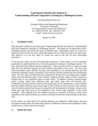
  • 9. has elements of both an initiating agent and a responding agent, and is thus subject to more diversity and utility. 4.3.Experiment 1 vs. Experiment 2: Graphs Appendix C documents the graphs of the agents’ learning record, before the second stage of agents’ life cycle. In general, the graphs reflect what we have discussed in Section 4.2. However, Figure 1 provides additional insights. From Figure 1, we see that utility of the casebase drops after reaching a high value. This is probably due to the convergence. After learning steadily, an agent hits Phase 3, the precision learning or the refinement learning phase, as shown in Figure 1. At this phase, the agent learns additional new cases to replace similar, used cases. Each replacement means removing a case with a nonzero value in #timesOfUsed, and adding a case with a zero value in #timesOfUsed. Since the utility of the casebase relies on the values of #timesOfUsed, the utility thus drops. However, it is assuring to see that the utility of the casebase goes up after each drop, meaning that the agent does learn useful cases. 4.4.Experiment 1 vs. Experiment 2: Impact of Different Initial Casebases, Second Stage This is the same as the experiments conducted in Section 4.4 of our previous report. Briefly, the goal of this second stage is to study the impact of different initial casebases. For the first stage, all agents start with the exactly same casebase. For the second stage, however, each casebase is different. First, we collect the casebases C f after running the first stage of the experiments. Then, from these casebases, we manually remove unused, pre-existing cases. In addition, remember that in Experiment 1, the agents use a combine learning: both self and cooperative learning; and in Experiment 2, the agents use only self-learning. Tables 6 and 7 document the results of completing the second stages of our experiments. Figures 1-4 in Appendix D supplements the results. From Table 6, in Experiment 1, the utility slope is lower than that in Experiment 2: 0.085 vs. 0.09125, but the average utility gain is higher than that in Experiment 2: 0.1325 vs. 0.09125. That is, the agents tend to learn differently in terms of utility given different initial casebases to start with. (Juan, the utility slope for Experiment 1, A1, is very high: 0.67!!! And its average utility gain is also 0.67!!! Very high!!! Please CHECK TO MAKE SURE THE NUMBERS ARE CORRECT.) I checked the number again and found that I input these two numbers wrong, the correct numbers are: 0.0652 for utility slope and 0.0674 for average utility gain. I chang the data in Table 6 and recalculate the average. However, Experiment 2 does offer a higher difference slope: 0.04125 vs. 0.035. This indicates that in Experiment 2, the agents are starting to introduce new blood into their own casebases, which they build on their own. Meanwhile, the agents in Experiment 1, though still incorporating foreign cases, do not inject more difference as they start with initial casebases grown from both self and cooperative learning. This observation on difference slope values is the same as reported in Section 4.4 of our previous report. From Table 7, Experiment 2 has a higher utility slope and a higher utility gain than Experiment 1: 0.1875 vs. 0.15125, and 0.1775 vs. 0.11, respectively. That indicates that for responding 9
  • 10. casebases, the agents that start with initial casebases grown using self-learning are able to learn more useful cases. This observation is different from what is reported in our previous report, in which Experiment 1 had a higher utility slope and a higher utility gain than Experiment 2. (This has to be studied further to find out what the justification is. The only difference in setup is agent A1. But looking at Table 7, A1 behaves normally. So, this particular item of result reported here, and the corresponding one reported in our previous report may simply be coincidental!!! So, we need to study this further.) In table 7, the contribution that leads to that Experiment 2 has a higher utility slope and average gain is mostly from A1 and A2. A1: utility slope 0.25 (self), 0.2 (coop). A1: average utility gain 0.28 (self), 0.16 (coop). A2: utility slope 0.27 (self), 0.3 (coop). A1: average utility gain 0.26 (self), 0.2 (coop). These two sets of numbers are much higher than other agents and agents in Experiment 1. I don’t understand that you say “looking at Table 7, A1 behaves normally” Doest it mean A1 should have high utility slope & average utility gain in Experiment 2 than in Experiment 1? If yes, then it is possible that the high utility slop and average utility gain of A1 leads to Experiment 2 has a higher utility slope and a higher utility gain than Experiment 1. On the other hand, Experiment 2 has a higher difference slope and a higher difference gain than Experiment 1, 0.035 vs. 0, and 0.0375 vs. 0.02125, respectively. This observation supports what we have mentioned from Table 6. In general, we see that the combine learning at the second stage is able to bring in more diversity to the casebase when the initial casebase has been grown using self-learning. Size Slope Difference Utility Slope Ave. Utility Ave. Diff. Slope Gain Gain Experiment 1 A1 Self 0.12 0.02 0.07 0.07 0.13 Combine-first- Coop 0.43 0.07 0.06 0.08 0.09 combine-later A2 Self 0.13 0.02 0.1 0.08 0.11 Coop 0.2 0.03 0.1 0.4 0.04 A3 Self 0.21 0.04 0.1 0.09 0.11 Coop 0.24 0.04 0.09 0.27 0.07 A4 Self 0.19 0.03 0.1 0.13 0.16 Coop 0.2 0.03 0.06 -0.06 0.07 average 0.2150 0.0350 0.085 0.1325 0.0975 Experiment 2 A1 Self 0.12 0.03 0.08 0.08 0.06 Self-first- Coop 0.21 0.06 0.05 0.06 0.14 combine-later A2 Self 0.21 0.06 0.08 0.08 0.14 Coop 0.2 0.05 0.09 0.09 0.03 A3 Self 0.13 0.04 0.12 0.11 0.06 Coop 0.13 0.04 0.09 0.26 0.1 A4 Self 0.14 0.02 0.12 0.13 0.1 Coop 0.06 0.03 0.1 -0.08 0.06 average 0.1500 0.0413 0.0913 0.0913 0.0863 Table 6 Utility and difference gains for both Experiments 1 and 2, after the second stage, for initiating casebases. 10
  • 11. Size Slope Difference Utility Slope Ave. Utility Ave. Diff. Slope Gain Gain Experiment 1 A1 Self 0.24 0.04 0.18 0.19 0.04 Combine-first- Coop 0.29 0.04 0.14 0.13 0.05 combine-later A2 Self 0.13 -0.02 0.14 0.18 -0.04 Coop 0.22 -0.01 0.16 -0.03 0.07 A3 Self 0.13 0.02 0.19 0.21 0.01 Coop 0.17 0.03 0.19 0.11 0.06 A4 Self 0.05 -0.08 0.11 0.13 -0.03 Coop 0.06 -0.02 0.1 -0.04 0.01 average 0.1613 0 0.1513 0.1100 0.0213 Experiment 2 A1 Self 0.31 0.06 0.25 0.28 0.06 Self-first- Coop 0.27 0.05 0.2 0.16 0.06 combine-later A2 Self 0.18 0.03 0.27 0.3 0.03 Coop 0.17 0.03 0.26 0.2 0.04 A3 Self 0.11 0.03 0.16 0.21 0.03 Coop 0.1 0.02 0.16 0.06 0.03 A4 Self 0.13 0.03 0.1 0.11 0.03 Coop 0.15 0.03 0.1 0.1 0.02 average 0.1775 0.035 0.1875 0.1775 0.0375 Table 7 Utility and difference gains for both Experiments 1 and 2, after the second stage, for responding casebases. Table 8 shows the number of unused, pre-existing cases that are deleted/replaced during the experiments. Once again, we see that the responding casebases encounter more deletions and replacements, as documented in our previous report as well. Combine-First-Combine-Later Self-First-Combine-Later Agent First Stage Second Stage First Stage Second Stage Ini Res Ini Res Ini Res Ini Res A1 0 0 0 0 0 0 0 0 A2 0 5 0 3 2 0 0 0 A3 0 2 0 0 0 4 0 0 A4 3 7 0 0 0 3 0 7 Table 8 The number of deleted/replaced unused, pre-existing cases. 5. DIFFERENCES BETWEEN PREVIOUS REPORT AND THIS REPORT Previously, we dealt with initial casebases of the same size (=16). In this report, we deal with three initial casebase with 16 cases and one with only 2 cases. The agent A1 with only 2 cases in its initial casebase has observable impact on both its own learning behavior and also on the overall system’s casebase quality. 1. For the experiments described in this report, in the initiating casebase, the cooperative learning has a much higher average utility gain. That is, the utility gain after each cooperative learning attempt is higher than that after each self-learning attempt. This is not so when we consider the responding casebase. In the previous report, the cooperative learning has lower average utility gain for both initiating case base and responding case base. 11
  • 12. That is, the utility gain after each cooperative learning attempt is lower than that after each self-learning attempt. This is due to the particular learning behavior of agent A1 as reported earlier in this document. 2. Each experiment has two stages. In our previous report, the utility slope and the average utility gain about the same for both experiments. That is, the utility-related statistics are t he same regardless of how the initial casebase for the second stage is grown. In this current report, however, we see that the utility slope and the average utility gain are higher in Experiment 1 than in Experiment 2, for initiating casebases, and lower for responding casebases. We attribute the difference for initiating casebases to how agent A1 reacts with a very small casebase to its environment. And the apparent “flip-flop” in observations for the responding casebases for the two reports we attribute it to possibly coincidental due to the fact that the responding cases are more diverse to begin with. We need to study this further. 6. CONCLUSIONS AND FUTURE WORK In this report, we have conducted further experiments to understand the role of self and cooperative learning in a multiagent system. Overall, we observe the same patterns and trends as those reported in our previous reports. Thus, in general, the size of the initial casebase does not impact the learning behavior of the overall system too significantly. However, we do see some changes in the utility quality and difference quality of the cases within the system due to the particular learning behavior of the agent with a very small casebase. The agent with a very small casebase is able to improve the utility of its casebase faster than the other agents as it stores cases that are more likely to be used. Also, the agent with a very small casebase is able to improve the diversity of its casebase faster than the other agents since its cooperative learning has a higher chance to bring in very different cases. For our next experiments, we will setup agents with very large casebases and average-sized casebases to see how the agents behave in such an environment. 12
  • 13. APPENDIX A: GAINS FOR EXPERIMENT 1: Combine-First-Combine-Later. Table 1(Initiating) Table 1(responding) Self Cooperative Self Cooperative #learnings 42 5 #learnings 30 10 #new cases 11 4 #new cases 11 3 avg util gain 0.1641 -0.0898 avg util gain 0.3469 -0.1078 max util gain 2.5 0.2721 max util gain 2.2222 0.7143 min util gain -0.85 -0.4167 min util gain -1 -0.7958 #util gain>0.400000 9 0 #util gain>0.400000 13 2 #util gain<-0.200000 6 2 #util gain<-0.200000 8 3 avg diff gain 0.0686 0.1428 avg diff gain 0.0683 0.0593 max diff gain 0.5891 0.2309 max diff gain 0.3543 0.1993 min diff gain 0 -0.0021 min diff gain 0 0 #diff gain>0.400000 1 0 #diff gain>0.400000 0 0 #diff gain<-0.200000 0 0 #diff gain<-0.200000 0 0 sizeslope 0.3261 0.3333 sizeslope 0.3514 0.359 difslope 0.0653 0.0651 difslope 0.0639 0.0662 utislope 0.1256 0.0882 utislope 0.2551 0.242 Table 1 Utility and difference gains for Agent A1, performing both learning mechanisms in Experiment Table 1(Initiating) Table 1(responding) Self Cooperative Self Cooperative #learnings 35 3 #learnings 33 11 #new cases 11 1 #new cases 13 1 avg util gain 0.0618 0.1842 avg util gain 0.0792 0.205 max util gain 0.5556 0.2906 max util gain 0.9357 0.5555 min util gain -0.1005 0.0952 min util gain -0.6667 0 #util gain>0.400000 1 0 #util gain>0.400000 5 2 #util gain<-0.200000 0 0 #util gain<-0.200000 4 0 avg diff gain 0.1935 0.0546 avg diff gain 0.0519 -0.0384 max diff gain 4.6464 0.1638 max diff gain 0.3073 0.228 min diff gain 0 0 min diff gain -0.3914 -0.3445 #diff gain>0.400000 1 0 #diff gain>0.400000 0 0 #diff gain<-0.200000 0 0 #diff gain<-0.200000 3 2 sizeslope 0.2973 0.3 sizeslope 0.3023 0.3158 difslope 0.0619 0.061 difslope 0.0288 0.0245 utislope 0.067 0.0651 utislope 0.1114 0.0974 Table 2 Utility and difference gains for Agent A2, performing both learning mechanisms in Experiment 13
  • 14. Table 1(Initiating) Table 1(responding) Self Cooperative Self Cooperative #learnings 47 4 #learnings 28 9 #new cases 10 2 #new cases 11 3 avg util gain 0.0941 0.0105 avg util gain 0.1445 0.1047 Max util gain 0.5556 0.2222 max util gain 0.5229 0.3846 min util gain -0.1082 -0.1087 min util gain -1 -0.1082 #util gain>0.400000 7 0 #util gain>0.400000 3 0 #util gain<-0.200000 0 0 #util gain<-0.200000 2 0 avg diff gain 0.1452 0.0796 avg diff gain 0.0659 0.06 Max diff gain 4.6213 0.16 max diff gain 0.4066 0.2006 min diff gain 0 0 min diff gain -0.2904 -0.0012 #diff gain>0.400000 1 0 #diff gain>0.400000 1 0 #diff gain<-0.200000 0 0 #diff gain<-0.200000 2 0 sizeslope 0.22 0.1714 sizeslope 0.3611 0.3077 difslope 0.0505 0.0438 difslope 0.0644 0.0519 utislope 0.0869 0.0893 utislope 0.1346 0.178 Table 3 Utility and difference gains for Agent A3, performing both learning mechanisms in Experiment Table 1(Initiating) Table 1(responding) Self Cooperative Self Cooperative #learnings 40 3 #learnings 35 12 #new cases 12 2 #new cases 12 2 avg util gain 0.0703 0.1628 avg util gain 0.152 0.1092 Max util gain 0.549 0.3518 max util gain 0.9524 0.4545 min util gain -0.1123 0 min util gain -1 -0.2254 #util gain>0.400000 2 0 #util gain>0.400000 3 1 #util gain<-0.200000 0 0 #util gain<-0.200000 1 1 avg diff gain 0.1536 0.0211 avg diff gain 0.0317 0.0136 Max diff gain 4.6234 0.1825 max diff gain 0.4254 0.2055 min diff gain -0.3766 -0.2747 min diff gain -0.4266 -0.2509 #diff gain>0.400000 2 0 #diff gain>0.400000 1 0 #diff gain<-0.200000 2 1 #diff gain<-0.200000 4 1 sizeslope 0.3095 0.3889 sizeslope 0.2889 0.2381 difslope 0.0377 0.0603 difslope 0.0271 0.0146 utislope 0.0758 0.0355 utislope 0.144 0.1361 Table 4 Utility and difference gains for Agent A4, performing both learning mechanisms in Experiment 14
  • 15. APPENDIX B: GAINS FOR EXPERIMENT 2: Self-First-Combine-Later. Table 1(Initiating) Table 1(responding) Self Self #learnings 51 #learnings 55 #new cases 11 #new cases 9 Avg util gain 0.1499 avg util gain 0.6867 Max util gain 2.3333 max util gain 5 Min util gain -0.6607 min util gain -1.3 #util gain>0.400000 9 #util gain>0.400000 37 #util gain<-0.200000 4 #util gain<-0.200000 6 Avg diff gain 0.0491 avg diff gain 0.0257 Max diff gain 0.5768 max diff gain 0.3056 Min diff gain 0 min diff gain 0 #diff gain>0.400000 1 #diff gain>0.400000 0 #diff gain<-0.200000 0 #diff gain<-0.200000 0 sizeslope 0.22 sizeslope 0.1667 difslope 0.0386 difslope 0.0257 utislope 0.1395 utislope 0.6867 Table 1 Utility and difference gains for Agent A1, performing only self learning in Experiment 2. Table 1(Initiating) Table 1(responding) Self Self #learnings 94 #learnings 41 #new cases 14 #new cases 10 Avg util gain 0.0422 avg util gain 0.3238 Max util gain 0.5029 max util gain 0.8333 Min util gain -1.3333 min util gain -0.13 #util gain>0.400000 3 #util gain>0.400000 14 #util gain<-0.200000 4 #util gain<-0.200000 0 Avg diff gain 0.068 avg diff gain 0.0531 Max diff gain 4.6372 max diff gain 0.3264 Min diff gain -0.3418 min diff gain 0 #diff gain>0.400000 1 #diff gain>0.400000 0 #diff gain<-0.200000 2 #diff gain<-0.200000 0 sizeslope 0.1398 sizeslope 0.225 difslope 0.0188 difslope 0.0531 utislope 0.0414 utislope 0.3238 Table 2 Utility and difference gains for Agent A2, performing only self learning in Experiment 2. 15
  • 16. Table 1(Initiating) Table 1(responding) Self Self #learnings 61 #learnings 58 #new cases 11 #new cases 14 avg util gain 0.0941 avg util gain 0.1347 max util gain 0.5359 max util gain 1.1111 min util gain -0.2029 min util gain -2.6667 #util gain>0.400000 9 #util gain>0.400000 8 #util gain<-0.200000 1 #util gain<-0.200000 5 avg diff gain 0.1014 avg diff gain 0.0298 max diff gain 4.4849 max diff gain 0.3338 min diff gain 0 min diff gain -0.356 #diff gain>0.400000 1 #diff gain>0.400000 0 #diff gain<-0.200000 0 #diff gain<-0.200000 4 sizeslope 0.1667 sizeslope 0.2281 difslope 0.0284 difslope 0.0298 utislope 0.0898 utislope 0.1347 Table 3 Utility and difference gains for Agent A3, performing only self learning in Experiment 2. Table 1(Initiating) Table 1(responding) Self Self #learnings 60 #learnings 54 #new cases 14 #new cases 14 avg util gain 0.0311 avg util gain 0.1367 max util gain 0.5425 max util gain 0.9524 min util gain -1 min util gain -4 #util gain>0.400000 2 #util gain>0.400000 16 #util gain<-0.200000 2 #util gain<-0.200000 6 avg diff gain 0.1177 avg diff gain 0.0336 max diff gain 4.5872 max diff gain 0.2782 min diff gain 0 min diff gain -0.3704 #diff gain>0.400000 1 #diff gain>0.400000 0 #diff gain<-0.200000 0 #diff gain<-0.200000 3 sizeslope 0.2203 sizeslope 0.2453 difslope 0.042 difslope 0.0336 utislope 0.0277 utislope 0.1367 Table 4 Utility and difference gains for Agent A4, performing only self learning in Experiment 2. 16
  • 17. APPENDIX C: EXPERIMENT 1 vs. EXPERIMENT 2: Graphs agent 1 ini size agent 1 res size 30 30 25 25 20 20 15 15 10 10 5 5 0 0 0 20 40 60 80 100 0 20 40 60 80 100 agent 2 ini size agent 2 res size 30 30 25 25 20 20 15 15 10 10 5 5 0 0 0 20 40 60 80 100 0 20 40 60 80 100 agent 3 ini size agent 3 res size 30 30 25 25 20 20 15 15 10 10 5 5 0 0 0 20 40 60 80 100 0 20 40 60 80 100 agent 4 ini size agent 4 res size 30 30 25 25 20 20 15 15 10 10 5 5 0 0 0 20 40 60 80 100 0 20 40 60 80 100 Figure 1 The number of cases in the casebase vs. time, in Experiment 1, before the second stage. 17
  • 18. agent 1 ini utility Agent 1 res utility 14 14 12 12 10 10 8 8 6 6 4 4 2 2 0 0 0 20 40 60 80 100 0 20 40 60 80 100 agent 2 ini utility agent 2 res utility 14 14 12 12 10 10 8 8 6 6 4 4 2 2 0 0 0 20 40 60 80 100 0 20 40 60 80 100 agent 3 ini utility agent 3 res utility 14 14 12 12 10 10 8 8 6 6 4 4 2 2 0 0 0 20 40 60 80 100 0 20 40 60 80 100 agent 4 ini utility agent 4 res utility 14 14 12 12 10 10 8 8 6 6 4 4 2 2 0 0 0 20 40 60 80 100 0 20 40 60 80 100 Figure 2 Utility gains vs. time for Experiment 1, before the second stage. 18
  • 19. agent 1 ini utility agent 1 res utility 14 14 12 12 10 10 8 8 6 6 4 4 2 2 0 0 0 20 40 60 80 100 0 20 40 60 80 100 agent 2 ini utility agent 2 res utility 14 14 12 12 10 10 8 8 6 6 4 4 2 2 0 0 0 20 40 60 80 100 0 20 40 60 80 100 agent 3 ini utility agent 3 res utility 14 14 12 12 10 10 8 8 6 6 4 4 2 2 0 0 0 20 40 60 80 100 0 20 40 60 80 100 agent 4 ini utility agent 4 res utility 14 14 12 12 10 10 8 8 6 6 4 4 2 2 0 0 0 20 40 60 80 100 0 20 40 60 80 100 Figure 3 Utility gains vs. time for Experiment 2, before the second stage. 19
  • 20. agent 1 ini size agent 1 res size 30 30 25 25 20 20 15 15 10 10 5 5 0 0 0 20 40 60 80 100 0 20 40 60 80 100 agent 2 ini size agent 2 res size 30 30 25 25 20 20 15 15 10 10 5 5 0 0 0 20 40 60 80 100 0 20 40 60 80 100 agent 3 ini size agent 3 res size 30 30 25 25 20 20 15 15 10 10 5 5 0 0 0 20 40 60 80 100 0 20 40 60 80 100 agent 4 ini size agent 4 res size 30 30 25 25 20 20 15 15 10 10 5 5 0 0 0 20 40 60 80 100 0 20 40 60 80 100 Figure 4 The number of cases in the casebase vs. time in Experiment 2, before the second stage. 20
  • 21. APPENDIX D: EXPERIMENT 1 vs. EXPERIMENT 2: Different Initial Casebases. agent 1 ini size agent 1 res size 30 30 25 25 20 20 15 15 10 10 5 5 0 0 0 10 20 30 40 50 60 70 80 0 10 20 30 40 50 60 70 80 agent 2 ini size agent 2 res size 30 30 25 25 20 20 15 15 10 10 5 5 0 0 0 10 20 30 40 50 60 70 80 0 10 20 30 40 50 60 70 80 agent 3 ini size agent 3 res size 30 30 25 25 20 20 15 15 10 10 5 5 0 0 0 10 20 30 40 50 60 70 80 0 10 20 30 40 50 60 70 80 agent 4 ini size agent 4 res size 30 30 25 25 20 20 15 15 10 10 5 5 0 0 0 10 20 30 40 50 60 70 80 0 10 20 30 40 50 60 70 80 Figure 1 The number of cases in the casebase vs. time, in Experiment 1, after the second stage. 21
  • 22. agent 1 ini utility agent 1 res utility 14 14 12 12 10 10 8 8 6 6 4 4 2 2 0 0 0 10 20 30 40 50 60 70 80 0 10 20 30 40 50 60 70 80 agent 2 ini utility agent 2 res utility 14 14 12 12 10 10 8 8 6 6 4 4 2 2 0 0 0 10 20 30 40 50 60 70 80 0 10 20 30 40 50 60 70 80 agent 3 ini utility agent 3 res utility 14 14 12 12 10 10 8 8 6 6 4 4 2 2 0 0 0 10 20 30 40 50 60 70 80 0 10 20 30 40 50 60 70 80 agent 4 ini utility agent 4 res utility 14 14 12 12 10 10 8 8 6 6 4 4 2 2 0 0 0 10 20 30 40 50 60 70 80 0 10 20 30 40 50 60 70 80 Figure 2 Utility gains vs. time for Experiment 1, after the second stage. 22
  • 23. agent 1 ini size agent 1 res size 30 30 25 25 20 20 15 15 10 10 5 5 0 0 0 10 20 30 40 50 60 70 80 0 10 20 30 40 50 60 70 80 agent 2 ini size agent 2 res size 30 30 25 25 20 20 15 15 10 10 5 5 0 0 0 10 20 30 40 50 60 70 80 0 10 20 30 40 50 60 70 80 agent 3 ini size agent 3 res size 30 30 25 25 20 20 15 15 10 10 5 5 0 0 0 10 20 30 40 50 60 70 80 0 10 20 30 40 50 60 70 80 agent 4 ini size agent 4 res size 30 30 25 25 20 20 15 15 10 10 5 5 0 0 0 10 20 30 40 50 60 70 80 0 10 20 30 40 50 60 70 80 Figure 3 The number of cases in the casebase vs. time in Experiment 2, after the second stage. 23
  • 24. agent 1 ini utility agent 1 res utility 14 14 12 12 10 10 8 8 6 6 4 4 2 2 0 0 0 10 20 30 40 50 60 70 80 0 10 20 30 40 50 60 70 80 agent 2 ini utility agent 2 res utility 14 14 12 12 10 10 8 8 6 6 4 4 2 2 0 0 0 10 20 30 40 50 60 70 80 0 10 20 30 40 50 60 70 80 agent 3 ini utility agent 3 res utility 14 14 12 12 10 10 8 8 6 6 4 4 2 2 0 0 0 10 20 30 40 50 60 70 80 0 10 20 30 40 50 60 70 80 agent 4 ini utility agent 4 res utility 14 14 12 12 10 10 8 8 6 6 4 4 2 2 0 0 0 10 20 30 40 50 60 70 80 0 10 20 30 40 50 60 70 80 Figure 4 Utility gains vs. time for Experiment 2, after the second stage. 24
  • 25. 25