Missing Parts: I don’t think you understood the assignment. I am looking at it, all I see is where you entered SAS codes and then that’s it. These SAS codes you inputted, I’d like to see some results, such as these things I am about to mention: Part I) 1. (2 pts.) Import the data into your software. Be sure to check that your data looks exactly like the original data before proceeding! 2. (2 pts.) For BOTH of your original quantitative variables, create TWO categorized versions based upon cutoffs of your choice. One binary version and one multi-level version with 3-5 groups. Use numbers for the new variables to represent the groups. No group should have less than 10% of the overall sample. Be sure you define your groups so that they do not overlap and you do not miss any observations. • In SPSS this can be done using TRANSFORM and RECODE INTO DIFFERENT VARIABLE. • In SAS you need to use a DATA step with IF-THEN statements to create the new variables. 3. (2 pts.) Create translations which provide the range of values for the variables created in Question 3. • In SPSS this is done in the variable view using the “Values” column. • In SAS you need to create the formats using PROC FORMAT and then assign those formats to the appropriate variables using a DATA step. 4. (3 pts.) Label all variables with descriptive titles. • In SPSS this is done in the variable view using the “Label” column. • In SAS you need to use a DATA step which includes a LABEL statement. All the codes I’m looking at, I didn’t need to see them, I expect to see them in a table. I’ve similar exercises, and that’s not how they look. PART II) Part 2: Descriptive Summary of Each Variable 5. (6 pts.) Calculate the sample size, sample mean, sample median, sample standard deviation, min, max, Q1, Q3, and 95% confidence interval for the population mean for your two quantitative variables. Provide the software output containing these results in your solution. 6. (6 pts.) Construct a histogram, boxplot, and QQ-plot for your two quantitative variables. Provide only the graphs in your solution. 7. (8 pts.) Construct a frequency table for each of the four variables created in Question 3. 8. (6 pts.) Provide a brief discussion of the distribution of your two main variables using as much of the information in Questions 5-7 as possible (and yet remain as concise as possible). Where did you do all these calculations; I didn’t see anything. I did see a histogram, that’s all I saw. Where’s the box plot, QQ plot, there was no graph. Also, you didn’t provide any discussion. PART III) Part 3: Case QQ - Using the two quantitative variables 9. (2 pts.) Construct a scatterplot. Provide only this plot in your solution. 10. (2 pts.) Regardless of whether it is appropriate, calculate Pearson’s correlation coefficient. Provide the output containing the estimate and the p-value. 11. (3 pts.) Regardless of whether it is a ...

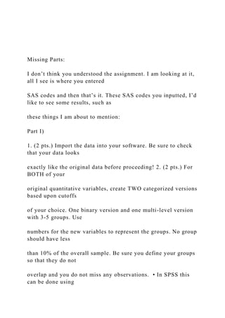
1. Missing Parts:
I don’t think you understood the assignment. I am looking at it,
all I see is where you entered
SAS codes and then that’s it. These SAS codes you inputted, I’d
like to see some results, such as
these things I am about to mention:
Part I)
1. (2 pts.) Import the data into your software. Be sure to check
that your data looks
exactly like the original data before proceeding! 2. (2 pts.) For
BOTH of your
original quantitative variables, create TWO categorized versions
based upon cutoffs
of your choice. One binary version and one multi-level version
with 3-5 groups. Use
numbers for the new variables to represent the groups. No group
should have less
than 10% of the overall sample. Be sure you define your groups
so that they do not
overlap and you do not miss any observations. • In SPSS this
can be done using

2. TRANSFORM and RECODE INTO DIFFERENT VARIABLE. •
In SAS you need
to use a DATA step with IF-THEN statements to create the new
variables. 3. (2 pts.)
Create translations which provide the range of values for the
variables created in
Question 3. • In SPSS this is done in the variable view using the
“Values” column. •
In SAS you need to create the formats using PROC FORMAT
and then assign those
formats to the appropriate variables using a DATA step. 4. (3
pts.) Label all
variables with descriptive titles. • In SPSS this is done in the
variable view using the
“Label” column. • In SAS you need to use a DATA step which
includes a LABEL
statement.
All the codes I’m looking at, I didn’t need to see them, I expect
to see them in a table. I’ve
similar exercises, and that’s not how they look.
PART II)
Part 2: Descriptive Summary of Each Variable 5. (6 pts.)
Calculate the sample size, sample

3. mean, sample median, sample standard deviation, min, max, Q1,
Q3, and 95% confidence
interval for the population mean for your two quantitative
variables. Provide the software
output containing these results in your solution. 6. (6 pts.)
Construct a histogram, boxplot,
and QQ-plot for your two quantitative variables. Provide only
the graphs in your solution.
7. (8 pts.) Construct a frequency table for each of the four
variables created in Question 3.
8. (6 pts.) Provide a brief discussion of the distribution of your
two main variables using as
much of the information in Questions 5-7 as possible (and yet
remain as concise as
possible).
Where did you do all these calculations; I didn’t see anything. I
did see a histogram, that’s all I
saw. Where’s the box plot, QQ plot, there was no graph. Also,
you didn’t provide any discussion.
PART III)
Part 3: Case QQ - Using the two quantitative variables 9. (2

4. pts.) Construct a scatterplot.
Provide only this plot in your solution. 10. (2 pts.) Regardless
of whether it is appropriate,
calculate Pearson’s correlation coefficient. Provide the output
containing the estimate and
the p-value. 11. (3 pts.) Regardless of whether it is appropriate,
conduct a simple linear
regression analysis. In your solution provide output containing:
overall ANOVA table,
table of parameter estimates (slope/intercept) including
confidence intervals, and the value
of the coefficient of determination, R2. Provide a histogram and
normal probability plot of
the residuals as well as a scatterplot of the residuals (Y) vs. the
predicted values (X) 12. (6
pts.) Provide a brief discussion of the relationship between your
two quantitative variables
using as much of the information in Questions 9-11 as possible.
• If linear regression and
correlation are appropriate, provide interpretations of the
correlation coefficient, the slope,
and the coefficient of determination • If these are not
appropriate, discuss why using as
much support as possible from your output and discuss whether

5. Spearman’s rank
correlation would be appropriate
First, where’s the scatter plot, missing. Where did you calculate
“r”? Very incomplete.
Part 4:
Case CC 13. (8 pts.) Construct all four combinations of two-
way tables which investigate
the relationship between your two variables. Your solution must
include the two-way table,
the row and column percentages, and the appropriate chi-
squared statistic with p-value.
14. (6 pts.) Provide a summary of the conclusions of the
appropriate chi-squared test for
each of the combinations in Question 13 including a discussion
of the distribution of your
response within the levels of the explanatory variable. Be sure
to address any concerns with
using these test.
I am gonna stop here, what you have is completely different
than what the teacher asked. I’m
completely unsatisfied, and franckly, I cannot release any fund
for that.

6. Below is an example of one of my homework. Take a look at it.
The SAS System
The FREQ Procedure
High blood pressure
HBP Frequency Percent Cumulative
Frequency
Cumulative
Percent
0 768 76.80 768 76.80
1 232 23.20 1000 100.00
Smoking Status
SMOKE Frequency Percent Cumulative
Frequency
Cumulative
Percent

7. 1 501 50.10 501 50.10
2 245 24.50 746 74.60
3 254 25.40 1000 100.00
The SAS System
The FREQ Procedure
High blood pressure
HBP Frequency Percent Cumulative
Frequency
Cumulative
Percent
0 768 76.80 768 76.80
1 232 23.20 1000 100.00
Smoking Status
SMOKE Frequency Percent Cumulative
Frequency

8. Cumulative
Percent
1 501 50.10 501 50.10
2 245 24.50 746 74.60
3 254 25.40 1000 100.00
The SAS System
The MEANS Procedure
Analysis Variable : AGE Age (years)
High
blood
pressur
e
N
Ob
s

9. N Mean Minimum Lower
Quartile
Median Upper
Quartile
Std Dev
0 768 76
8
43.842447
9
20.000000
0
29.000000
0
40.000000
0
56.000000
0
17.669939

10. 9
1 232 23
2
66.956896
6
29.000000
0
58.000000
0
68.000000
0
77.000000
0
13.808769
6

11. The SAS System
The FREQ Procedure
High blood pressure
HBP Frequency Percent Cumulative
Frequency
Cumulative
Percent
0 768 76.80 768 76.80
1 232 23.20 1000 100.00
Smoking Status
SMOKE Frequency Percent Cumulative
Frequency
Cumulative
Percent
1 501 50.10 501 50.10
2 245 24.50 746 74.60
3 254 25.40 1000 100.00

12. The SAS System
The MEANS Procedure
Analysis Variable : AGE Age (years)
High
blood
pressur
e
N
Ob
s
N Mean Minimum Lower
Quartile
Median Upper
Quartile
Std Dev

13. 0 768 76
8
43.842447
9
20.000000
0
29.000000
0
40.000000
0
56.000000
0
17.669939
9
1 232 23
2
66.956896
6

14. 29.000000
0
58.000000
0
68.000000
0
77.000000
0
13.808769
6
The SAS System
The MEANS Procedure
Analysis Variable : AGE Age (years)
Smokin
g Status

15. N
Ob
s
N Mean Minimum Lower
Quartile
Median Upper
Quartile
Std Dev
1 501 50
1
47.646706
6
20.000000
0
30.000000
0
42.000000
0

16. 64.000000
0
20.288443
4
2 245 24
5
58.265306
1
20.000000
0
45.000000
0
61.000000
0
73.000000
0
17.709143
1

17. 3 254 25
4
43.539370
1
20.000000
0
30.000000
0
40.000000
0
55.000000
0
16.262071
4
The SAS System

18. The FREQ Procedure
High blood pressure
HBP Frequency Percent Cumulative
Frequency
Cumulative
Percent
0 768 76.80 768 76.80
1 232 23.20 1000 100.00
Smoking Status
SMOKE Frequency Percent Cumulative
Frequency
Cumulative
Percent
1 501 50.10 501 50.10
2 245 24.50 746 74.60
3 254 25.40 1000 100.00

19. The SAS System
The MEANS Procedure
Analysis Variable : AGE Age (years)
High
blood
pressur
e
N
Ob
s
N Mean Minimum Lower
Quartile
Median Upper
Quartile
Std Dev
0 768 76
8

20. 43.842447
9
20.000000
0
29.000000
0
40.000000
0
56.000000
0
17.669939
9
1 232 23
2
66.956896
6
29.000000
0

21. 58.000000
0
68.000000
0
77.000000
0
13.808769
6
The SAS System
The MEANS Procedure
Analysis Variable : AGE Age (years)
Smokin
g Status
N
Ob

22. s
N Mean Minimum Lower
Quartile
Median Upper
Quartile
Std Dev
1 501 50
1
47.646706
6
20.000000
0
30.000000
0
42.000000
0
64.000000
0

23. 20.288443
4
2 245 24
5
58.265306
1
20.000000
0
45.000000
0
61.000000
0
73.000000
0
17.709143
1
3 254 25
4

24. 43.539370
1
20.000000
0
30.000000
0
40.000000
0
55.000000
0
16.262071
4
The SAS System

25. The FREQ Procedure
High blood pressure
HBP Frequency Percent Cumulative
Frequency
Cumulative
Percent
0 768 76.80 768 76.80
1 232 23.20 1000 100.00
Smoking Status
SMOKE Frequency Percent Cumulative
Frequency
Cumulative
Percent
1 501 50.10 501 50.10
2 245 24.50 746 74.60
3 254 25.40 1000 100.00

26. The SAS System
The MEANS Procedure
Analysis Variable : AGE Age (years)
High
blood
pressur
e
N
Ob
s
N Mean Minimum Lower
Quartile
Median Upper
Quartile
Std Dev
0 768 76

27. 8
43.842447
9
20.000000
0
29.000000
0
40.000000
0
56.000000
0
17.669939
9
1 232 23
2
66.956896
6
29.000000

28. 0
58.000000
0
68.000000
0
77.000000
0
13.808769
6
The SAS System
The MEANS Procedure
Analysis Variable : AGE Age (years)
Smokin
g Status
N

29. Ob
s
N Mean Minimum Lower
Quartile
Median Upper
Quartile
Std Dev
1 501 50
1
47.646706
6
20.000000
0
30.000000
0
42.000000
0
64.000000

30. 0
20.288443
4
2 245 24
5
58.265306
1
20.000000
0
45.000000
0
61.000000
0
73.000000
0
17.709143
1
3 254 25

31. 4
43.539370
1
20.000000
0
30.000000
0
40.000000
0
55.000000
0
16.262071
4

32. The SAS System
The FREQ Procedure
High blood pressure
HBP Frequency Percent Cumulative
Frequency
Cumulative
Percent
0 768 76.80 768 76.80
1 232 23.20 1000 100.00
Smoking Status
SMOKE Frequency Percent Cumulative
Frequency
Cumulative
Percent

33. 1 501 50.10 501 50.10
2 245 24.50 746 74.60
3 254 25.40 1000 100.00
The SAS System
The MEANS Procedure
Analysis Variable : AGE Age (years)
High
blood
pressur
e
N
Ob
s
N Mean Minimum Lower
Quartile

34. Median Upper
Quartile
Std Dev
0 768 76
8
43.842447
9
20.000000
0
29.000000
0
40.000000
0
56.000000
0
17.669939
9
1 232 23

35. 2
66.956896
6
29.000000
0
58.000000
0
68.000000
0
77.000000
0
13.808769
6
The SAS System
The MEANS Procedure

36. Analysis Variable : AGE Age (years)
Smokin
g Status
N
Ob
s
N Mean Minimum Lower
Quartile
Median Upper
Quartile
Std Dev
1 501 50
1
47.646706
6
20.000000
0
30.000000

37. 0
42.000000
0
64.000000
0
20.288443
4
2 245 24
5
58.265306
1
20.000000
0
45.000000
0
61.000000
0
73.000000

38. 0
17.709143
1
3 254 25
4
43.539370
1
20.000000
0
30.000000
0
40.000000
0
55.000000
0
16.262071
4

39. The SAS System
The FREQ Procedure
Frequency
Percent
Row Pct
Col Pct
Table of HBP by SMOKE
HBP(High blood pressure) SMOKE(Smoking Status)
1 2 3 Total
0 398
39.80
51.82
79.44

40. 155
15.50
20.18
63.27
215
21.50
27.99
84.65
768
76.80
1 103
10.30
44.40
20.56
90

41. 9.00
38.79
36.73
39
3.90
16.81
15.35
232
23.20
Total 501
50.10
245
24.50
254
25.40

42. 1000
100.00
The SAS System
The FREQ Procedure
Frequency
Percent
Row Pct
Col Pct
Table of HBP by SMOKE
HBP(High blood
pressure)
SMOKE(Smoking Status)

43. Former Current 3 Total
No 398
39.80
51.82
79.44
155
15.50
20.18
63.27
215
21.50
27.99
84.65
768
76.80
yes 103

44. 10.30
44.40
20.56
90
9.00
38.79
36.73
39
3.90
16.81
15.35
232
23.20
Total 501
50.10

45. 245
24.50
254
25.40
1000
100.00
The SAS System
The FREQ Procedure
Frequency
Percent
Row Pct
Col Pct

46. Table of HBP by SMOKE
HBP(High blood
pressure)
SMOKE(Smoking Status)
Never Former Current Total
No 398
39.80
51.82
79.44
155
15.50
20.18
63.27
215
21.50
27.99
84.65

47. 768
76.80
yes 103
10.30
44.40
20.56
90
9.00
38.79
36.73
39
3.90
16.81
15.35
232

48. 23.20
Total 501
50.10
245
24.50
254
25.40
1000
100.00
BIdAgeFEVHeightSex5095131.072460564231.40451.51515240.
8394801375141.5695001425241.5774904955141.102480547514
1.3894807595141.4184902384140.7964714054141.7895218084
141.004481435151.4490515151.25652.50685151.282490725351
.6125201045151.3435001515351.5365202855151.19646.503335
150.7915203925151.5525404294151.7045104455151.14650046

49. 15151.0925006415251.5895107205251.539500354151.4725016
04251.7555211004151.7765111124152.01754.511574151.85853
11584251.4525111884451.5852.513994151.8195314734151.971
5814974151.80855.517444151.935117464151.35950.517654151
.5145218384152.115501175261.919580175361.415560195261.6
02530355161.8785301425161.4815101615161.7195301625261.
6955304365162.10255.504805261.6975505365161.33851.50576
5161.7965505834161.5235106235161.3435207424161.5355508
175161.6725401084161.655511224161.6345411454161.74757.5
12394161.9795612484361.7185512944361.3385313254261.572
5213274261.3485313364161.4315113434161.52752.513824261.
5364813974161.71350.513984161.62451.514564161.666521456
4261.82652.514664162.26257.514664262.10456.515134161.423
49.517124161.7155317494161.6995418034161.6915318124161.
42749.5150171.7254.50725272.09357.501370172.41960014651
71.63155.501625172.1115701665171.9175802485171.74258.50
2500171.6035102520171.8295402795271.47352.502850171.698
54.502915171.82754.502940171.4615402995471.60951.503815
271.755504705371.695404755272.0955704950171.7265305360
171.375506025171.41553.506160171.72856.506415171.645507
200171.87752.507205171.93552.507465272.00257.507575172.3
665807790172.5645808380172.37155.508395271.49557031427
1.932531520172.57862.511070171.6245411570171.7895611850
171.2535212084171.61157.512344271.6825512380171.6495412
700172.0845812740172.225812900172.2195513350171.905581
3914172.0465614000171.6585314050172.15853.514324271.165
4714450171.7953.514504171.7965514840171.9256.515494171.
61256.516420172.0565417144472.555617440172.13556177141
72.53559.518140171.82651145181.72467.50170182.336610190
181.98758.50210182.19358.50610182.98600725182.673600850
182.1755901040181.9315701075181.34452.501405181.69857.5
01420182.4816001530182.5315801810182.1446302155282.215
6002220182.3886002365381.2925202505282.63959.502845282.
34160.502880181.87256.502970181.6975903000182.458610327
5182.28861.503510282.2935803720182.6656403920181.7858.5
03930181.9535804470182.18761.504525181.33556.504565382.

50. 70962.504730182.14559.504930182.9936304975182.30564.505
070181.55658.505130181.5125305495282.1355906005182.3355
906190181.84456.506310282.4766306410182.3826207315182.3
586107590182.0696007650182.3335707675181.7585208060181
.99956.508270182.01557.508390182.328600200181.735541240
182.11860.51310282.258581910182.071551920181.5475719301
82.004571980182.425911120182.73260.511220181.70354.5114
10182.1236011450181.945911524181.9625711650182.2116311
660181.79454.512364181.5235512440182.35458.512960182.09
5712974181.5625513100181.42957.513150181.6755313250182.
0695413560182.92763.513824181.7595313990182.6315914220
182.5036315154281.99159.515210181.89755.515420182.01656
15564582.68160.515790182.015515860181.74452.516110182.4
3559.516264182.3035717000182.2265717140182.63159173342
82.09457.517570182.55718000181.6245318150181.6575613019
1.708570195191.942600560192.988650680192.1600950193.135
6001060192.0765701150192.79761.501335193.01662.50152019
2.5660.502015293.02961.502390292.57460.502990192.0455.50
3155191.94756.503360192.4636103380192.6316203510393.042
6603805192.59260.503880192.25958.503900192.04864.503980
192.8516004210193.0046404250191.9335804255292.09158.504
290192.31659.504320191.60657.504390192.325704700192.166
57.504810192.4556004890192.135904940192.5295904954292.4
4261.504970192.0566305050191.9695905470192.63963055652
93.2236505860292.4856406180192.856306230191.75461.50704
0191.8865607185191.9125907460192.18259.507830192.487640
7835291.5915708145192.68859.5064291.55853190191.8955714
20192.352591430192.60461.51570292.34860172019365.518801
92.7255911200193.5566211240292.575711460192.0695811540
192.7156011544392.4575911560192.0959.511610193.84269118
84392.65961.511940192.1266212080192.96464.512290192.196
6112310191.7515812344192.16561.512380292.5886312910192.
425713004392.6563.513330191.77358.513410193.11464.51343
0192.13558.513730192.30158.513790192.466413910192.57160.
513940192.89364.514420192.236114430191.71655.514500192.
71761.514530192.1195714610192.8716514724292.97359.51484

51. 0292.1646015124192.0426215150193.6816816080192.07660.51
6270292.24663.516320193.2396516394192.45761.517110192.8
3361.517250192.80359.517300192.9236417420191.8556018030
192.7986218080191.869571
Part 2: Descriptive Summary of Each Variable
5. (6 pts.) Calculate the sample size, sample mean, sample
median, sample standard deviation, min, max, Q1,
Q3, and 95% confidence interval for the population mean for
your two quantitative variables. Provide the
software output containing these results in your solution.
6. (6 pts.) Construct a histogram, boxplot, and QQ-plot for your
two quantitative variables. Provide only the
graphs in your solution.
7. (8 pts.) Construct a frequency table for each of the four
variables created in Question 3.
8. (6 pts.) Provide a brief discussion of the distribution of your
two main variables using as much of the
information in Questions 5-7 as possible (and yet remain as
concise as possible).
Part 3: Case QQ - Using the two quantitative variables
9. (2 pts.) Construct a scatterplot. Provide only this plot in your
solution.
10. (2 pts.) Regardless of whether it is appropriate, calculate
Pearson’s correlation coefficient. Provide the

52. output containing the estimate and the p-value.
11. (3 pts.) Regardless of whether it is appropriate, conduct a
simple linear regression analysis. In your solution
provide output containing: overall ANOVA table, table of
parameter estimates (slope/intercept) including
confidence intervals, and the value of the coefficient of
determination, R2. Provide a histogram and normal
probability plot of the residuals as well as a scatterplot of the
residuals (Y) vs. the predicted values (X)
12. (6 pts.) Provide a brief discussion of the relationship
between your two quantitative variables using as much
of the information in Questions 9-11 as possible.
• If linear regression and correlation are appropriate, provide
interpretations of the correlation
coefficient, the slope, and the coefficient of determination
• If these are not appropriate, discuss why using as much
support as possible from your output and
discuss whether Spearman’s rank correlation would be
appropriate
Part 4: Case CC
13. (8 pts.) Construct all four combinations of two-way tables
which investigate the relationship between your
two variables. Your solution must include the two-way table,
the row and column percentages, and the
appropriate chi-squared statistic with p-value.
14. (6 pts.) Provide a summary of the conclusions of the
appropriate chi-squared test for each of the
combinations in Question 13 including a discussion of the

53. distribution of your response within the levels of
the explanatory variable. Be sure to address any concerns with
using these tests.
Part 5: Case CQ
15. (2 pts.) Construct side-by-side boxplots of your chosen
response variable by the binary version of your
explanatory variable. Provide only the graph in your solution.
16. (4 pts.) Conduct a two-sample t-test. Provide all output
given by your software in your solution.
17. (6 pts.) Provide a conclusion about the relationship between
your two variables based upon the results in
Questions 15 and 16. Be sure to state which t-test you are using
and interpret the confidence interval for the
difference between the two population means. Address any
concerns with using this test.
Part 6: Case CQ
18. (2 pts.) Construct side-by-side boxplots of your chosen
response variable by the multi-level version of your
explanatory variable. Provide only the graph in your solution.
19. (4 pts.) Conduct an ANOVA. Provide only the basic
ANOVA table in your solution.
20. (6 pts.) Provide a conclusion about the relationship between
your two variables based upon the results in
Questions 18 and 19. Address any concerns with using this test.
Part 7: Summary
21. (10 pts.) Compare the results of the different ways of
investigating the relationship between your two
variables. Did all of the conclusions agree? What type(s) of
error(s) might you have made for each of the

54. tests? What are the strengths and limitations of each method?
Learning Objectives
CO-4: Distinguish among different measurement scales, choose
the appropriate descriptive and inferential statistical
methods based on these distinctions, and interpret the results.
LO 4.3: Using appropriate numerical measures and/or visual
displays, describe the distribution of a categorical variable in
context.
LO 4.4: Using appropriate graphical displays and/or numerical
measures, describe the distribution of a quantitative variable
in context: a) describe the overall pattern, b) describe striking
deviations from the pattern.
LO 4.7: Define and describe the features of the distribution of
one quantitative variable (shape, center, spread, outliers).
LO 4.8: Define and calculate the sample mean of a quantitative
variable.
LO 4.9: Define and calculate the sample median of a
quantitative variable.
LO 4.10: Choose the appropriate measures for a quantitative
variable based upon the shape of the distribution.
LO 4.12: Define and calculate Q1, Q3, and the IQR for one
quantitative variable.
LO 4.13: Define and calculate the standard deviation and
variance of one quantitative variable.
LO 4.14: Define and interpret measures of position (percentiles,
quartiles, the five-number summary, z-scores).
LO 4.18: Compare and contrast distributions (of quantitative
data) from two or more groups, and produce a brief summary,
interpreting your findings in context.
LO 4.19: For a data analysis situation involving two variables,
identify the role of each variable in the scenario.
LO 4.20: Classify a data analysis situation involving two
variables according to the “role-type classification.”

55. LO 4.21: For a data analysis situation involving two variables,
determine the appropriate graphical display(s) and/or
numerical measures(s) that should be used to summarize the
data.
LO 4.23: Given a contingency table (two-way table), interpret
the information it reveals about the association between two
categorical variables by calculating and comparing conditional
percentages.
LO 4.25: Describe the relationship displayed in a scatterplot
including: a) the overall pattern, b) striking deviations from the
pattern.
LO 4.26: Explain the limitations of Pearson’s correlation
coefficient (r) as a measure of the association between two
quantitative variables.
LO 4.27: In the special case of a linear relationship, interpret
Pearson’s correlation coefficient (r) in context.
LO 4.28: In the special case of a linear relationship, interpret
the slope of the regression line and use the regression line to
make predictions.
LO 4.29: Determine and use the correct point estimates for
specified population parameters.
LO 4.30: Interpret confidence intervals for population
parameters in context.
LO 4.36: For a data analysis situation involving two variables,
carry out the appropriate inferential method for examining
relationships between the variables and draw the correct
conclusions in context.
LO 4.38: In a given context, determine the appropriate standard
method for comparing groups and provide the correct
conclusions given the appropriate software output.
LO 4.39: In a given context, set up the appropriate null and
alternative hypotheses for comparing groups.
LO 4.41: Based upon the output for a two-sample t-test,
correctly interpret in context the appropriate confidence interval
for the difference between population means.
LO 4.42: Based upon the output for a two-sample t-test,

56. determine whether to use the results assuming equal variances
or
those assuming unequal variances.
LO 4.43: In a given context, determine the appropriate standard
method for examining the relationship between two
categorical variables. Given the appropriate software output,
choose the correct p-value and provide the correct
conclusions in context.
LO 4.44: In a given context, set up the appropriate null and
alternative hypotheses for examining the relationship between
two categorical variables.
LO 4.45: In a given context, set up the appropriate null and
alternative hypotheses for examining the relationship between
two quantitative variables.
LO 4.46: In a given context, determine the appropriate standard
method for examining the relationship between two
quantitative variables and interpret the results provided in the
appropriate software output in context.
LO 4.47: For simple linear regression models, interpret the
coefficient of determination in context.
CO-5: Determine preferred methodological alternatives to
commonly used statistical methods when assumptions are not
met.
LO 5.1: For a data analysis situation involving two variables,
determine the appropriate alternative (non-parametric)
method when assumptions of our standard methods are not met.
LO 5.2: Recognize situations in which Spearman’s rank
correlation is a more appropriate measure of the relationship
between two quantitative variables.
CO-6: Apply basic concepts of probability, random variation,
and commonly used statistical probability distributions.
LO 6.1: Explain the meaning of the term distribution in
statistics.

57. LO 6.3: Use histograms and QQ-plots (or Normal Probability
Plots) to visually assess the normality of distributions of
quantitative variables.
LO 6.4: Relate the probability of an event to the likelihood of
this event occurring.
LO 6.5: Apply the relative frequency approach to estimate the
probability of an event.
LO 6.9: Apply logic or probability rules to calculate conditional
probabilities, P(A|B), and interpret them in context.
LO 6.19: Identify and distinguish between a parameter and a
statistic.
LO 6.27: Explain what the p-value is and how it is used to draw
conclusions.
LO 6.28: Define a Type I and Type II error in general and in the
context of specific scenarios.
LO 6.30: Use a confidence interval to determine the correct
conclusion to the associated two-sided hypothesis test.
CO-7: Use statistical software to analyze public health data.
LO 7.0: Apply other software skills such as labeling variables,
creating translations for coded categorical variables, and
creating new variables.
LO 7.1: View a dataset in EXCEL, text editor, or other
spreadsheet or statistical software.
LO 7.2: Given data containing a categorical variable, use
software to create a frequency distribution, bar chart, and pie
chart.
LO 7.3: Given data containing a quantitative variable, use
software to create a histogram, boxplot, and QQ-plot (or PP-
Plot).
LO 7.4: Given data containing a quantitative variable, use
software to calculate numerical summaries.
LO 7.5: Given appropriate data involving two variables, use
software to construct side-by-side boxplots.
LO 7.6: Given appropriate data involving two variables, use
software to calculate numerical measures for a quantitative
variable within two or more groups.

58. LO 7.7: Given appropriate data involving two variables, use
software to construct a two-way table.
LO 7.8: Given appropriate data involving two variables, use
software to construct a scatterplot.
LO 7.9: Given appropriate data involving two variables, use
software to calculate the value of Pearson’s correlation
coefficient.
LO 7.10: Given appropriate data involving two variables, use
software to calculate the value of the coefficient of
determination (R-squared).
LO 7.11: In the special case of a linear relationship, use
software to construct the simple linear regression equation.
LO 7.15: Given appropriate data, use software to conduct a two-
sample t-test.
LO 7.16: Given appropriate data, use software to conduct an
ANOVA.
LO 7.17: Given appropriate data, use software to conduct a chi-
square test of independence of two categorical variables.
LO 7.18: Given appropriate data, use software to conduct a test
for statistical significance of Pearson’s correlation
coefficient.
LO 7.19: Given appropriate data, use software to conduct a test
for statistical significance of the slope of the simple linear
regression equation.
CO-8: Develop presentations based on statistical analyses for
both public health professionals and educated lay
audiences.
There are no learning sub-objectives for this course objective.
This course objective will be assessed through group and
individual assignments during the semester.
hggyuA(10)