1. By: Kawar Abid
The Round Turbulent Jet
Objective:
The purpose of this experiment to study the behavior of turbulent air
flow that exit from round pipe and to know the velocity profile of the jet that
exits from that pipe.
Introduction:
The behavior of a jet as it mixes into the fluid which surrounding it
has importance in many engineering applications. The exhaust from a gas
turbine or cars is an obvious example. In this experiment we establish the
shape of an air jet as it mixes in a turbulent manner with the surrounding air.
If the Reynolds number of a jet is sufficiently small, the jet remains laminar
for some length. In this case the mixing with the surrounding fluid is very
slight, and the jet retains its identity. Laminar jets are important in certain
fluidic applications, where a typical diameter of pipe may be equal to 1 mm.
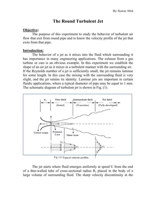
The schematic diagram of turbulent jet is shown in Fig. (1).
The jet starts where fluid emerges uniformly at speed U from the end
of a thin-walled tube of cross-sectional radius R, placed in the body of a
large volume of surrounding fluid. The sharp velocity discontinuity at the
Fig. (1)
2. By: Kawar Abid
edge of the tube gives rise to an annular shear layer which almost
immediately becomes turbulent.
The width of a viscous layer increases in the downstream direction as
shown in that diagram. For a short distance from the end of the tube the
layer does not extend right across the jet, so that at section 1 there is a core
of fluid moving with the undisturbed velocity U at the inside. Further
downstream the shear layer extends right across the jet and the velocity uo on
the jet axis starts to fall as the mixing continues until ultimately the motion
is completely dissipated.
Description of Apparatus and Procedure:
The round jet is produced by discharging air from the air box through
a short tube as indicated in Fig.(2). The inlet of the tube is rounded to
prevent separation so that a basically uniform velocity distribution is
produced at the tube exit.
A travel across mechanism is supported on the tube so that a pitot tube may
be brought to any desired position in the jet. Measurements are normally
made in one plane.
Fig. (2)
The pitot tube is first brought into the plane of the exit of the jet tube
and the scale readings are noted for which the axial position (X=0) and the
radial position (r=0) are zero. The latter may be obtained by taking the
average of the readings when the tube is set in line with one side and then
3. By: Kawar Abid
the other side of the tube. The pressure Po in the air box is then brought to a
convenient value and traverses are made at various axial stations along the
length of the jet.
Theory:
The atmospheric pressure at Duhok city is equal to 950 mbar, or
2
/
95000 m
N
patm = , and the temperature of air inside the duct is equal to15 o
C,
then the absolute temperature of air is equal to 288K. So the air density is
can be calculated using the ideal gas law as follows:
T
R
p air
= …………………………………………………………..(1.1)
Or:
3
/
14
.
1
)
273
15
(
287
96000
m
kg
=
+
=
…………………………………………(1.2)
The total pressure can be measured at end of pipe by using fine Pitot tube
and manometer as follows:
H
P water
t
= ……………………………………………………………(1.3)
Where: H is the manometer pressure head in mm.
The uniform velocity V in (m/s) at end of tube can be estimated as follows:
2
2
1
V
Pt
= ……………………………………………………….……(1.4)
Then the Reynolds number at end section of the pipe is equal to:
D
V
=
Re …………………………………………………………..….(1.5)
Where is the air kinematic viscosity (m2
/s).
The pressure values (Po) at different (X) sections can be measured by using
fine pitot tube and manometers as follows:
2
2
1
o
o v
P
= ………………………………………………………….…(1.6)
While, the pressure values (P) at different (r) sections can be measured by
using fine pitot tube and manometers as follows:
2
2
1
v
P
= ………………………………………………………….…(1.7)
4. By: Kawar Abid
Sample of Calculations:
Diameter of tube, D= 51.6 mm.
Radius of tube, R=25.8 mm.
Kinematic viscosity, υ =1.48×10⁻⁵
m2
/s. ……….. Constant
Total head, H = mm,
Total pressure, =
= H
P water
Uniform velocity, 2
2
1
V
P
=
Then, V
2p
= =
Readings and Results:
Table (1) Velocity distribution along a center line of the jet (X) .
X ↓
(mm)
h
(mm)
p
(N/m)
v
(m/s)
𝑣
𝑉
0
50
100
150
200
250
300
350
400
Notes: All elevations or pressure readings (h) must subtracted from (100 mm).
Table (2) Velocity distribution at various (r) sections of the jet.
r
mm
X=75 mm X=150 mm X=225 mm X=300 mm X=375 mm
h
mm
𝑣
𝑣o
h
mm
𝑣
𝑣o
h
mm
𝑣
𝑣o
h
mm
𝑣
𝑣o
h
mm
𝑣
𝑣o
0
10
20
30
40
50
60
70
80