Constant Temperature Boundaries in 1. Rectangular Plate 2. T-shaped Plate

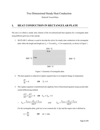
1. Page 1 of 9
Two Dimensional Steady Heat Conduction
Shehzaib Yousuf Khan
1. HEAT CONDUCTION IN RECTANGULAR PLATE
The aim is to obtain a steady state solution of the two-dimensional heat equation for a rectangular plate
using different grid sizes of Δ𝑥 and Δ𝑦.
1. MATLAB © software is used to develop the solver for steady state conduction in the rectangular
plate where the length and height are 𝐿𝑥 = 5 𝑚 and 𝐿𝑦 = 2 𝑚 respectively, as shown in Figure 1.
Figure 1: Geometry of rectangular plate.
2. The heat equation is reduced to Laplace equation due to no temporal change in temperature.
𝜕𝑇
𝜕𝑡
= 0 𝑶𝑹 𝑇𝑡 = 0
3. The Laplace equation is transformed into algebraic form of discretised equation using second order
central differencing method.
𝜕2
𝑇
𝜕𝑥2
+
𝜕2
𝑇
𝜕𝑦2
= 0 𝑶𝑹 𝑇𝑥𝑥 + 𝑇𝑦𝑦 = 0
∴ 𝑇𝑥𝑥 =
𝑇𝑖+1,𝑗 − 2𝑇𝑖,𝑗 + 𝑇𝑖−1,𝑗
(Δ𝑥)2
𝑎𝑛𝑑 𝑇𝑦𝑦 =
𝑇𝑖,𝑗+1 − 2𝑇𝑖,𝑗 + 𝑇𝑖,𝑗−1
(Δ𝑦)2
For the rectangular plate, grid size is not constant (Δ𝑥 ≠ Δ𝑦) and the aspect ratio is defined as:
𝛼 =
Δ𝑥
Δ𝑦
𝑶𝑹 𝛥𝑥 = 𝛼Δ𝑦

2. Page 2 of 9
The discretised equation becomes,
𝑇𝑖+1,𝑗 − 2𝑇𝑖,𝑗 + 𝑇𝑖−1,𝑗
(Δ𝑥)2
+
𝑇𝑖,𝑗+1 − 2𝑇𝑖,𝑗 + 𝑇𝑖,𝑗−1
(Δ𝑦)2
+ 𝒪(Δ𝑥2
, Δ𝑦2) = 0
𝑇𝑖+1,𝑗 − 2𝑇𝑖,𝑗 + 𝑇𝑖−1,𝑗
(Δ𝑥)2
+
𝑇𝑖,𝑗+1 − 2𝑇𝑖,𝑗 + 𝑇𝑖,𝑗−1
(Δ𝑦)2
~ 0
𝑇𝑖+1,𝑗 − 2𝑇𝑖,𝑗 + 𝑇𝑖−1,𝑗 + (
Δ𝑥
Δ𝑦
)
2
(𝑇𝑖,𝑗+1 − 2𝑇𝑖,𝑗 + 𝑇𝑖,𝑗−1) ~ 0
𝑇𝑖+1,𝑗 − 2𝑇𝑖,𝑗 + 𝑇𝑖−1,𝑗 + 𝛼2
(𝑇𝑖,𝑗+1 − 2𝑇𝑖,𝑗 + 𝑇𝑖,𝑗−1) ~ 0
𝑇𝑖+1,𝑗 + 𝑇𝑖−1,𝑗 + 𝛼2
(𝑇𝑖,𝑗+1 + 𝑇𝑖,𝑗−1) ~ 2𝑇𝑖,𝑗 + 2𝛼2
𝑇𝑖,𝑗
The temperature distribution is therefore can be estimated from the neighbouring nodes, which is
solved by forming a set of elements in a matrix.
𝑇𝑖,𝑗 ~
𝑇𝑖+1,𝑗 + 𝑇𝑖−1,𝑗 + 𝛼2
(𝑇𝑖,𝑗+1 + 𝑇𝑖,𝑗−1)
2 + 2𝛼2
4. Initially, a matrix of zeros is formed with a finite number of elements 𝑁𝑥 and 𝑁𝑦 which is related
to the grid size in respective spatial coordinates (𝑥, 𝑦). The node numbering has one extra element
at the top and right boundaries as shown in Figure 2.
𝑁𝑥 =
𝐿𝑥
Δ𝑥
; 𝑁𝑦 =
𝐿𝑦
Δ𝑦
Figure 2: Double index (𝑖, 𝑗) node numbering.
N + N + N +
N +

3. Page 3 of 9
5. The boundary conditions for the rectangular plate are given as:
a. Top: 𝑇(𝑥, 𝐿𝑦) = 350℃
b. Left: 𝑇(0, 𝑦) = 300℃
c. Right: 𝑇(𝐿𝑥, 𝑦) = 300℃
d. Bottom: 𝑇(𝑥, 𝐿𝑦) = 300℃
The boundary conditions are set in such a way that the interior nodes are not disturbed.
• The top edge of the plate is at 𝑦 = 𝑁𝑦 + 1 from 𝑥 = 1 to 𝑁𝑥 + 1.
• The bottom edge of the plate is at 𝑦 = 1 from 𝑥 = 1 to 𝑁𝑥 + 1.
• The left edge of the plate is at 𝑥 = 1 from 𝑦 = 1 to 𝑁𝑦 + 1.
• The right edge of the plate is at 𝑥 = 𝑁𝑥 + 1 from 𝑦 = 1 to 𝑁𝑦 + 1.
The interior nodes are from 𝑥 = 2 to 𝑁𝑥 and 𝑦 = 2 to 𝑁𝑦. Example:
𝑇2,2 ~
𝑇3,2 + 𝑇1,2 + 𝛼2
(𝑇2,3 + 𝑇2,1)
2 + 𝛼2
⇒ 𝑇2,2 ~
𝑇3,2 + 𝑇𝑟𝑖𝑔ℎ𝑡 + 𝛼2
(𝑇2,3 + 𝑇𝑏𝑜𝑡𝑡𝑜𝑚)
2 + 2𝛼2
6. Iterative method with stopping criteria is selected for converging the solution with tolerance of
1 × 10−6
and while loop is used for Error reaching the Tolerance.:
𝐸𝑟𝑟𝑜𝑟 = max(max(|𝑇 − 𝑇𝑜𝑙𝑑|))
7. For loop is used to solve the matrix for temperature of interior node.
8. The surface and contour plots are obtained for the temperature distribution in the rectangular plate.
Figure 3: Contour plot of temperature distribution in the rectangular plate.
2

4. Page 4 of 9
Figure 4: Surface plot of temperature distribution in the rectangular plate.
MATLAB CODE
clear all; clc;
% Geometry of Rectangular Plate
%
% _________________________
% | |
% | |
% | |
% Ly | |
% | |
% | |
% |_________________________|
% Lx
%
Lx = 5; Ly = 3;
% Grid
Nx = 100; Ny = 100; % Number of Elements
dx = Lx/Nx; dy = Ly/Ny; % Element Size
alpha = dx/dy; % Aspect ratio of element
% Spatial Locations
x = 0:dx:Lx; y = 0:dy:Ly;
% Boundary Conditions
Ttop = 350;
Tleft = 300;
Tright = 300;
Tbottom = 300;

5. Page 5 of 9
% Initial Conditions
T = zeros(Nx+1,Ny+1);
T(1:Nx+1,Ny+1) = Ttop;
T(1,1:Ny+1) = Tleft;
T(Nx+1,1:Ny+1) = Tright;
T(1:Nx+1,1) = Tbottom;
% Error Tolerance
tol = 1e-6; error = 1;
%Solver
counter = 1;
while (error>tol)
Told = T;
% FOR LOOP for interior nodes
for i=2:Nx
for j=2:Ny
T(i,j) = (T(i-1,j) + T(i+1,j) + (alpha^2)*(T(i,j-1) +
T(i,j+1)))/(2*(1+(alpha^2)));
end
end
% Stopping Criteria
error = max(max(abs(Told - T)));
counter = counter + 1;
end
T = T'; % Transpose
% Number of iterations
counter
% Contour Plot of Temperature Profile
figure(1)
contourf(x,y,T)
pbaspect([alpha 1 1]) % Aspect Ratio of Figure
xlabel('Length (m)'); ylabel('Height (m)');
colorbar
colormap(jet)
% Surface Plot of Temperature Profile
figure(2)
surf(x,y,T)
pbaspect([alpha 1 1]) % Aspect Ratio of Figure
xlabel('Length (m)'); ylabel('Height (m)');
colorbar
colormap(jet)

6. Page 6 of 9
2. HEAT CONDUCTION IN T-SHAPED PLATE
The aim is to obtain a steady state solution of the two-dimensional heat equation for a T-shaped plate using
grid sizes of Δ𝑥 and Δ𝑦.
1. MATLAB © software is used to develop the solver for steady state conduction in the T-shaped
plate where the geometry is separated in two blocks A and B. Figure 1 shows Block A of length
and height as 𝐿𝐴𝑥 = 0.5 𝑚 and 𝐿𝐴𝑦 = 1 𝑚, respectively. Also, there is Block B with length and
height as 𝐿𝐵𝑥 = 3 𝑚 and 𝐿𝐵𝑦 = 0.5 𝑚, respectively.
Figure 1: Geometry of rectangular plate.
2. The heat equation is reduced to Laplace equation due to no temporal change in temperature and
discretised using second order central differencing method. With constant grid size (Δ𝑥 = Δ𝑦), the
equation is transformed into algebraic form.
𝑇𝑖,𝑗 ~
𝑇𝑖+1,𝑗 + 𝑇𝑖−1,𝑗 + 𝑇𝑖,𝑗+1 + 𝑇𝑖,𝑗−1
4
3. Initially, a matrix of zeros is formed with a finite number of elements collectively for block A and
block B. Where, it is related to the grid size in respective spatial coordinates (𝑥, 𝑦).
𝑁𝐴𝑥 : Number of elements in a row of block A
𝑁𝐴𝑦 : Number of elements in a column of block A
𝑁𝐵𝑥 : Number of elements in a row of block A
𝑁𝐵𝑦 : Number of elements in a column of block A
𝑁𝐴𝑥 =
𝐿𝐴𝑥
Δ𝑥
; 𝑁𝐴𝑦 =
𝐿𝐴𝑦
Δ𝑦
; 𝑁𝐵𝑥 =
𝐿𝐵𝑥
Δ𝑥
; 𝑁𝐵𝑦 =
𝐿𝐵𝑦
Δ𝑦
The node numbering has one extra element at the top and right boundaries.

7. Page 7 of 9
4. The boundary conditions as shown in Figure 1 are set in such a way that the interior nodes are not
disturbed. For Block A:
• The top edge is at 𝑦 = 𝑁𝐴𝑦 + 1 from 𝑥 = 1 to 𝑁𝐴𝑥 + 1.
• The bottom edge is at 𝑦 = 1 from 𝑥 = 1 to 𝑁𝐴𝑥 + 1.
• The left edge is at 𝑥 = 1 from 𝑦 = 1 to 𝑁𝐴𝑦 + 1.
• The right edge is at 𝑥 = 𝑁𝐴𝑥 + 1 from 𝑦 = 1 to 𝑁𝐴𝑦 + 1.
For Block B: The position of bottom edge is set at a distance of Y elements. Whereas,
• The top edge is at 𝑦 = 𝑌 + 𝑁𝐴𝑦 + 1 from 𝑥 = 𝑁𝐴𝑥 + 1 to 𝑁𝐴𝑥 + 𝑁𝐵𝑥 + 1.
• The bottom edge is at 𝑦 = 𝑌 from 𝑥 = 𝑁𝐴𝑥 + 1 to 𝑁𝐴𝑥 + 𝑁𝐵𝑥 + 1.
• The left edge is at 𝑥 = 𝑁𝐴𝑥 + 1 from 𝑦 = 𝑌 to 𝑌 + 𝑁𝐵𝑦 + 1.
• The right edge is at 𝑥 = 𝑁𝐴𝑥 + 𝑁𝐵𝑥 + 1 from 𝑦 = 𝑌 to 𝑌 + 𝑁𝐵𝑦 + 1.
5. Iterative method with stopping criteria is selected for converging the solution with tolerance of
1 × 10−6
and while loop is used for Error reaching the Tolerance.:
𝐸𝑟𝑟𝑜𝑟 = max(max(|𝑇 − 𝑇𝑜𝑙𝑑|))
6. For loop is used to solve the matrix for temperature of interior nodes and interface nodes.
a. The interior nodes in block A from 𝑥 = 2 to 𝑁𝐴𝑥 and 𝑦 = 2 to 𝑁𝐴𝑦.
b. The interior nodes in block B from 𝑥 = 2 + 𝑁𝐴𝑥 to 𝑁𝐴𝑥 + 𝑁𝐵𝑥 and 𝑦 = 𝑌 + 1 to 𝑌 + 𝑁𝐵𝑦.
c. The interface nodes at 𝑥 = 𝑁𝐴𝑥 + 1 and 𝑦 = 𝑌 + 1 to 𝑌 + 𝑁𝐵𝑦.
7. The contour plot is obtained for the temperature distribution in the T-shaped plate.
Figure 2: Contour plot of temperature distribution in the T-shaped plate.

8. Page 8 of 9
MATLAB CODE
clear all; clc;
% Geometry of T-shaped Plate
%
% ___________
% | |
% | |_______________________
% | |
% LAy | | LBy
% | _______________________|
% | | LBx
% |___________|
% LAx
%
LAx = 0.5; LAy = 1; LBx = 2.5; LBy = 0.5;
% Grid
dx = 0.01; dy = dx; % Element size (Considering dx = dy)
% Number of Elements
NAx = LAx/dx; NAy = LAy/dy; NBx = LBx/dx; NBy = LBy/dy;
% Number of Elements at Interface of Block A and B
Y = (NAy-NBy)/2;
% Spatial Locations
x = 0 : dx : LAx+LBx;
y = 0 : dy : LAy;
% Boundary Conditions
TAtop = 300; TBtop = 300;
TAleft = 450; TBleft = 300;
TAright = 300; TBright = 300;
TAbottom = 300; TBbottom = 300;
% Initial Conditions
T = zeros(NAx+NBx+1,NAy+1);
% BLOCK A:
T(1:NAx+1,NAy+1) = TAtop;
T(1,1:NAy+1) = TAleft;
T(NAx+1,1:NAy+1) = TAright;
T(1:NAx+1,1) = TAbottom;
= TBtop;
= TBleft;
= TBright;
= TBbottom;
% BLOCK B:
T(NAx+1:NAx+NBx+1,Y+NBy+1)
T(NAx+1,Y:Y+NBy+1)
T(NAx+NBx+1,Y:Y+NBy+1)
T(NAx+1:NAx+NBx+1,Y) %
Error Tolerance
tol = 1e-6;
error = 1;
%Solver
counter = 1;
while (error>tol)
Told = T;
% FOR LOOP for interior nodes of A
for a = 2 : NAx

9. Page 9 of 9
for b = 2:NAy
T(a,b) = 0.25*(T(a-1,b) + T(a+1,b) + T(a,b-1) + T(a,b+1));
end
end
% FOR LOOP for interior nodes of B
for c = 2 + NAx : NAx + NBx
for d = Y + 1 : Y + NBy
T(c,d) = 0.25*(T(c-1,d) + T(c+1,d) + T(c,d-1) + T(c,d+1));
end
end
% FOR LOOP at the interface of block A and B
for e = NAx + 1
for f = Y + 1 : Y + NBy
T(e,f) = 0.25*(T(e-1,f) + T(e+1,f) + T(e,f-1) + T(e,f+1));
end
end
% Stopping Criteria
error = max(max(abs(Told - T)));
counter = counter + 1;
end
T(T==0) = nan; % Replace zeros with Null
T = T'; % Transpose
% Number of iterations
counter
% Contour Plot of Temperature Profile
contourf(x,y,T)
pbaspect([(LAx+LBx)/LAy 1 1]) % Aspect Ratio of Figure
xlabel('Length (m)'); ylabel('Height (m)');
colorbar
caxis([300 450])
colormap(jet)